Effects of study area size on home range estimates of common bottlenose dolphins Tursiops truncatus

Abstract

Knowledge of an animal’s home range is a crucial component in making informed management decisions. However, many home range studies are limited by study area size, and therefore may underestimate the size of the home range. In many cases, individuals have been shown to travel outside of the study area and utilize a larger area than estimated by the study design. In this study, data collected by multiple research groups studying bottlenose dolphins on the east coast of Florida were combined to determine how home range estimates increased with increasing study area size. Home range analyses utilized photo-identification data collected from 6 study areas throughout the St Johns River (SJR; Jacksonville, FL, USA) and adjacent waterways, extending a total of 253 km to the southern end of Mosquito Lagoon in the Indian River Lagoon Estuarine System. Univariate kernel density estimates (KDEs) were computed for individuals with 10 or more sightings (n = 20). Kernels were calculated for the primary study area (SJR) first, then additional kernels were calculated by combining the SJR and the next adjacent waterway; this continued in an additive fashion until all study areas were included. The 95% and 50% KDEs calculated for the SJR alone ranged from 21 to 35 km and 4 to 19 km, respectively. The 95% and 50% KDEs calculated for all combined study areas ranged from 116 to 217 km and 9 to 70 km, respectively. This study illustrates the degree to which home range may be underestimated by the use of limited study areas and demonstrates the benefits of conducting collaborative science.

The home range of an animal is defined as the area occupied by an individual during its everyday activities (Burt 1943). The area in which an animal spends 95% of its time is considered the home range, while the more concentrated area in which it spends 50% of its time is the core area (White and Garrot 1990). In general, the quantity and quality of resources within a habitat dictate the size of an animal’s home range and the areas of preferred use within it (Ballance 1992; Ingram and Rogan 2002; Hastie et al. 2004; Henry et al. 2005; Parra 2006). Ranging and habitat-use patterns are further influenced by factors such as predation risk (Heithaus and Dill 2002), anthropogenic activity (Bejder et al. 2006; Pirotta et al. 2013; Bas et al. 2014), physiological limitations (Williams et al. 1992), reproductive status (Henry et al. 2005; Gibson et al. 2013), and the behavior of both con- and hetero-specifics (Wilson et al. 1997; Parra 2006). For example, in terrestrial mammals, it has been shown that home ranges are generally larger for carnivores than for herbivores (Harestad and Bunnell 1979). In addition, home range sizes have been linked to the body size of an animal (McNab 1963; Garland 1983; Lindstedt et al. 1986). As bottlenose dolphins are one of the top marine predators and capable of swimming very efficiently, they are expected to have large home ranges (Ingram and Rogan 2002). Male bottlenose dolphins can weigh up to 500 kg and females up to 260 kg (Folkens et al. 2008). Terrestrial, carnivorous mammals of this size have a predicted home range of 396.03 km² for males and 214.18 km² for females (Lindstedt et al. 1986). Male bottlenose dolphins presumably have larger home ranges than females, which are thought to allow increased reproductive access to females (Eisenberg 1966; Wells et al. 1987; Wells 1991; Sprogis et al. 2015). Although locomotion constraints are typically limiting for terrestrial mammals, in an aquatic environment these restrictions are reduced; therefore, bottlenose dolphin home ranges, especially within relatively shallow habitats, can be larger for the same level of energetic costs (Williams et al. 1992; Connor et al. 2000).

Home range studies are typically conducted to provide data on the extent and area of habitat use in order to make spatial planning and management decisions, and potentially lead to the evaluation of anthropogenic impacts on populations (Merriman et al. 2009). However, one substantial limitation of such studies is that the area estimated to be the home range is often limited by the size of the study area (Zolman 2002; Merriman et al. 2009; Urian et al. 2009; Balmer et al. 2014). Many studies have used only the limited data from their study area to quantify home ranges, even though they have documented individuals traveling far beyond the boundaries of the study area (Gruber 1981; Hanby 2005; Fury and Harrison 2008). For example, Ingram and Rogan (2002) concluded from their study of bottlenose dolphins in the Shannon Estuary in Ireland that the study estuary did not encompass the entire geographical range of the population because the ranges of individuals did not reach an asymptote when all of their sightings were included. Similarly, it appears that a chosen study area in the Marlborough Sounds, New Zealand is only one important section of a larger home range as dolphins have been estimated to travel more than 80 km outside of the study area (Merriman et al. 2009). Thus, it is unlikely that the boundaries of a selected study area will encompass the entire home range of an individual dolphin (Davis 1953), as animals are not constrained by the study area boundaries.

Data on bottlenose dolphin home ranges have been based on study areas varying from 100 to 12,000 km², resulting in home range estimates ranging from 20 to 343.89 km², and the percent coverage (home range/study area× 100) ranging from 1.08% to 104% (Shane 1987; Connor et al. 2000; Gubbins 2002; Ingram and Rogan 2002; Lynn and Wursig 2002; Candido and Dos Santos 2005; Hanby 2005; Litz et al. 2007; Martinez-Serrano et al. 2011; Kiszka et al. 2012; Sprogis et al. 2015). In terms of linear distances, estuarine bottlenose dolphins have been reported to have maximum linear distances (MLDs) traveled along shoreline ranging from 12 to 105 km (Balmer et al. 2008). Thus, there is great variability in home range estimates currently available for bottlenose dolphins, which could be because funding and time often constrain the area a single research team can cover. Extending the boundaries of individual study areas into adjacent waterways, thereby covering more of an animal’s range, would enable better conservation and management of this species through improved knowledge of their movements (Ingram and Rogan 2002).

While previous research suggests that the size of the study area affects the estimate of home range, this study directly tested for a change in estimated home range size with increased study area. The Northeast Florida Dolphin Research Consortium (NEFL DRC), a collaboration among 8 research organizations with adjacent estuarine study areas, provides a unique opportunity to assess the impact of study area size on home range and core area estimates. Within the area covered by the consortium, there are currently two recognized estuarine stocks of bottlenose dolphins: the Jacksonville Estuarine System stock and the Indian River Lagoon Estuarine System stock (Waring et al. 2016). These two stocks are currently managed separately as rates of interchange are thought to be low. This research compares the home range and core area estimates from a 40-km linear study area within the St Johns River (SJR; Jacksonville, FL, USA) with the home range and core area estimates obtained by sequentially adding adjacent study areas, and ultimately including the consortium’s combined 253 km study area. Our primary aim is to determine the minimum study area size necessary to obtain valid ranging estimates for estuarine bottlenose dolphins.

Materials and Methods

Study area

The SJR served as the primary study area for this project. It spans nearly 500 km through Northeast Florida (DeMort 1991) and is a large brackish river with extensive boat traffic and shipping activity. The SJR intersects the Intracoastal Waterway (ICW; an inland waterway that runs north to south paralleling the coast) 8 km from the mouth of the river. Approximately 170 km to the south, the ICW converges with the Indian River Lagoon system. The individual study areas for these analyses consist of the SJR (40 km), the ICW south through Duval county (DUV; 55 km), the ICW south through St John’s county (SJC; 36 km), the ICW south through Flagler county (FL; 31 km), the ICW south to New Smyrna Beach (NSB; 48 km), and finally, south through the Mosquito Lagoon of the Indian River Lagoon Estuarine System (ML; 43 km) (Table 1 and Figure 1).

Table 1.

Length of each study area, additive lengths of combined study areas, and the total number of surveys conducted in each area

	Study Area
	SJR	DUV	SJC	FL	NSB	ML
Study area length (km)	40	55	36	31	48	43
Cumulative length (km)	–	95	131	162	210	253
Total number of surveys	71	23	17	18	41	19

Figure 1.

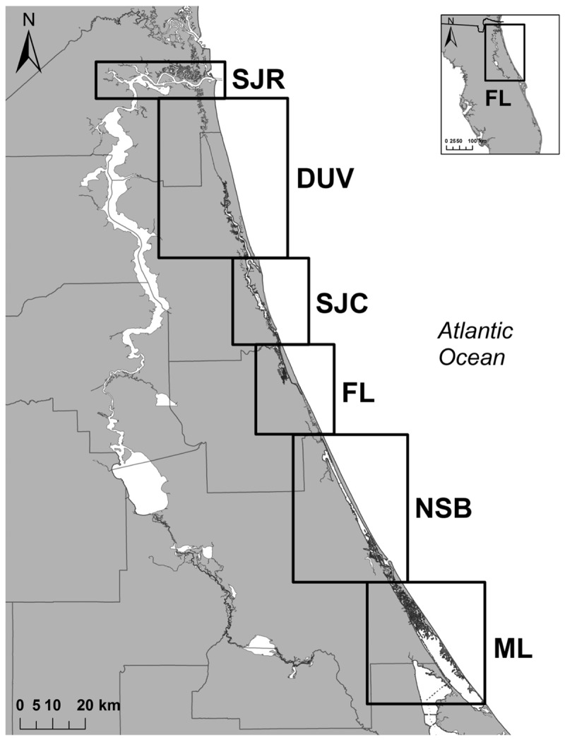
The 6 adjacent estuarine study areas: St Johns River (SJR), the Intracoastal Waterway (ICW) south through Duval County (DUV), the ICW south through St John’s county (SJC), the ICW south through Flagler county (FL), the ICW south to New Smyrna Beach (NSB), and south through the Mosquito Lagoon (ML).

Data collection

NEFL DRC was established in 2011 to coordinate research efforts in response to a bottlenose dolphin Unusual Mortality Event in the SJR. The initial goal of the consortium was to systematically survey bottlenose dolphins in Northeast Florida’s estuarine waters to determine abundance and rates of interchange between regions. During seasonal (winter/summer) coordinated surveys, each organization was responsible for surveying one section of the 253 km study area.

Each survey was conducted along a fixed survey route by a team of at least 3 personnel consisting of a boat driver, photographer, and data recorder. The vessel was operated at a speed of 10–12 km/h until dolphins were spotted, at which point the vessel was slowed to match the speed of the dolphins or stopped completely. Using a professional grade digital camera equipped with a 100–400 mm telephoto zoom lens, photographs were taken of the dorsal fins of each individual and the sighting location was recorded with a hand-held global positioning system (GPS). For each sighting, the minimum, maximum, and best field estimates were recorded for group size as well as the number of calves and young of the year.

Surveys were conducted from March 2011 to May 2012, but the frequency of surveys differed for each study area (Table 1). The SJR was surveyed on a weekly basis, with approximately 4 surveys a month. In DUV, SJC, and FL, surveys were conducted opportunistically, with a maximum of 4 surveys per season in DUV and 3 in SJC and FL. NSB was surveyed approximately twice monthly and in ML there were approximately 3 surveys every summer and every winter. An additional 12 coordinated consortium surveys were included from April 2012 to February 2014 for all areas except SJC and FL. Due to the variation in survey frequencies, analyses of home range were weighted based on effort in each area (see below for details).

Photo analysis

Individual dolphins were identified using standard photo-identification practices (Mazzoil et al. 2004). The best photograph of each individual from each sighting was selected and graded for quality. Quality was defined by focus, contrast, proportion of fin visible, proportion of frame filled by fin, and angle (Urian et al. 1999). Each photograph received a score of Q-1 (excellent quality), Q-2 (average quality), or Q-3 (poor quality). Only Q-1 and Q-2 photographs were included in analyses. All individuals then received a distinctiveness score of D-1 (very distinctive), D-2 (average distinctiveness), or D-3 (not distinctive) (Urian et al. 1999). Only individuals ranked as D-1 or D-2 were included in analyses. The photographs were then compared with the master catalog for the relevant study area and the sighting history for each individual was updated. If no match was found, the dolphin was entered as a new individual and given a new identification code. Photographs from the SJR catalog, excluding calves, were then matched against photographs provided by the other consortium organizations from the coordinated surveys. For matched individuals, all available sighting information from March 2011 to February 2014 was obtained, including data collected by member organizations during non-consortium surveys. These data were consolidated to create a detailed sighting history for each animal. Individuals were classified into three sex categories: female (F), male (M), and unknown (UNK). Females were individuals sighted with a calf in infant position (Mann et al. 2000) on at least 2 sightings. Individuals were categorized as males if they had been genetically sampled. Lastly, individuals that did not fall into either of those two categorizes were considered unknown sex.

Range calculations

First, individuals from the SJR catalog were selected (n = 288); 148 ranked as D-1, 113 as D-2, and 27 as D-3. D-3 animals were excluded from further analyses. Only individuals sighted 10 or more times, not including same day resights, were included in the analysis (n = 100; 39 F, 11 M, and 50 UNK). These data were used solely for home range analyses for the SJR individuals; because this data set included a large proportion of the SJR catalog, this analysis enabled a more accurate assessment of variation among individuals within the SJR study area.

For the remaining analyses, the data set was restricted to individuals from the SJR catalog that were also sighted outside of the SJR study area during collaborative consortium surveys (n = 27); 18 ranked as D-1, 9 as D-2, and none were ranked as D-3. It is important to note that the number of individuals sighted outside of the SJR is a conservative number as the entire catalog of each organization was not compared (i.e., the initial round of matching utilized data collected during consortium surveys only); thus, these data do not reflect the true rates of interchange between these regions. Of the selected individuals, only dolphins that were sighted 10 or more times were included in the analyses (n = 20; 7 F, 1 M, and 12 UNK). The mean sighting duration, time span between first and last sightings, of these individuals was 2.33 years (min: 1.61 years, max: 2.91 years).

Sighting histories of individuals with GPS location data were plotted in ArcGIS 10.1 (ESRI; Redlands, CA, USA). A midline was mapped throughout the entire geographic area covered, and the GPS locations were transformed onto the line using the “locate features along routes” function. The furthest upriver location that was surveyed in the SJR was defined as location zero. Distances from location zero were then computed for each of the sighting locations on the line, resulting in a univariate data set. Due to the fact that the end of the SJR does not lead into the next study area, but instead ends at the ocean, the midline through the SJR was truncated at the intersection with the ICW and continues south to the DUV study area (Figure 2). The intersection lies approximately 8 km west of the mouth of the river. Therefore, sightings east of the intersection were condensed onto the nearest point of the shortened midline. The decision was made to place location zero on the west side of the ICW intersection rather than at the mouth of the river because 80% of sightings in the SJR were located on the west side. Therefore, more sightings would have been condensed if location zero was set to the east side of the intersection. In order to assess the potential effects of this truncation; home range analyses were conducted for the SJR study area using both the shortened midline and a midline extending the full length of the study area; differences between the two estimates were then calculated.

Figure 2.

Map of the intersection between the SJR and the ICW south through DUV study areas, showing the location of the truncated SJR midline. The midline truncated at the SJR and DUV intersection is displayed by the arrow. Stars represent the start and end points of the SJR survey route.

Maximum linear distance

The MLD was calculated to determine the distance between the two most extreme sightings of each individual, without crossing land. Using the univariate data set produced in ArcGIS, MLDs were first calculated for individuals sighted 10 or more times in the SJR study area. The consortium data were then added following a sequential order from the SJR study area south; DUV, SJC, FL, NSB, and ML. When the number of sightings for each individual reached 10 or above, the MLD was computed using the combined sighting location data.

Home range analyses

Due to the high variability in home range estimates, a number of studies have been conducted that compare the precision and accuracy of the various home range estimators. The kernel density estimator (KDE) is considered the most robust (Hansteen et al. 1997), accurate, efficient (Borger et al. 2006), and beneficial test for home range analyses (Bowman and Azzalini 1997). Typically, home range studies have utilized bivariate data to estimate space use, not accounting for any barriers to the animal’s movements (Vokoun 2003) until after the polygons of space use are computed, at which point the unusable area is often removed (e.g., Fury and Harrison 2008; Gibson et al. 2013). However, the removal of uninhabitable area (i.e., land) from bivariate home range kernels is problematic because the proportion removed is not uniform across individuals. As an alternative, the use of univariate data for home range analyses is beneficial when studying a population that inhabits a narrow, aquatic environment. Spatial density calculation (Hanby 2005) is another potential method of limiting analyses to space that can be utilized by the animal, but in a narrow habitat, utilizing a second dimension in space is not necessarily more informative. Thus, the KDE was used in conjunction with univariate data as it allows for a more accurate analysis of home ranges (Moyer et al. 2007) in a linear estuarine environment. This method of analyzing univariate data with KDE has also been used to calculate alongshore home ranges of Hector’s dolphins (Cephalorhynchus hectori; Rayment et al. 2009).

Home ranges were first calculated for individuals sighted 10 or more times within the SJR study area. Then data from each additional study area were added following a sequential order. Once the number of sightings for each individual reached 10 or above, the home range was calculated using the combined sighting location data. Each sighting was weighted based on the survey effort in each study area (Equations 1 and 2; Rayment et al. 2009). Each study area was assigned a weight, $Wi$, which was calculated using Formula 1 where $Ai$ is the area of each section that was surveyed, $Vi$ the number of times that section was surveyed during the chosen time period, and $T$ the number of sections surveyed.

$$Wi=1/\frac{(Ai\times Vi)}{{\sum }_{i=1}^T(Ai\times Vi)}.$$

Each sighting then received a scaled weight, $W_i^S$, which was calculated using Formula 2 where $N$ is the total number of sightings for each individual.

$$W_i^S=\frac{Wi}{{\sum }_{i=1}^{N}Wi}.$$

The univariate data for each individual was input into program SAS (version 9.2; SAS Institute, Cary, NC, USA) and the function PROC KDE was used to compute the fixed 95% and 50% utilization KDE by incorporating the weights into the program. Three different computational methods for automatically selecting bandwidth were used: simple normal reference (SNR), Silverman’s rule of thumb (SROT), and the Sheather–Jones plug-in (SJPI). The resulting kernel density graphs were then compared. With an increase in sightings, the pattern between bandwidth smoothing methods became apparent (Figure 3). SROT undersmoothed the data and showed more of a bimodal distribution for many of the individuals. SNR and SJPI produced very similar graphs; however, SJPI oversmoothed and therefore obscured the underlying structure. SNR appeared to moderately smooth the data and was therefore used for all analyses. The home ranges for all individuals were first estimated utilizing only SJR data, then the adjacent study area’s data were added to SJR’s and the new home range was estimated. This continued progressively, north to south until all study areas were included.

Figure 3.

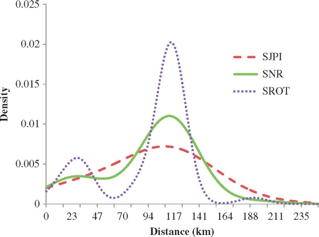
Univariate kernel density estimates for the distribution of sighting distances for bottlenose dolphins using the full 253 km study area. Three different bandwidth selection methods are shown: Sheather–Jones plug-in (SJPI), simple normal reference (SNR), and Silverman’s rule of thumb (SROT). SNR was selected for all analyses.

Results

Sightings

Twenty-seven distinctive individuals were sighted within and beyond the SJR study area, with an average of 8.44 sightings within the SJR (Table 2). One dolphin was sighted in 6 study areas, 2 dolphins were sighted in 5 study areas, 6 were sighted in 4 study areas, 8 were sighted in 3 study areas, and 10 were sighted in 2 study areas. However, these were not necessarily adjacent study areas. Of the individuals sighted in only two study areas, 50% of them were seen in SJR and ML, the two furthest locations in this study (Table 2).

Table 2.

Number of sightings for individual dolphins in each study area

		Study area
ID code	Sex	SJR	DUV	SJC	FL	NSB	ML
NAIA	F	17	1				1
NASA	UNK	16	3
KIAW	F	16					1
Q027	F	15	1	1			3
PUKA	F	15				2
Q142	UNK	14					1
LTUS	F	12	1			1	1
ZDCO	UNK	12					2
WIKD	M	11	1				1
Q080	F	10				2
Q144	UNK	9	1				1
Q158	F	8	2	1
SLPY	UNK	3	11
NUKK	UNK	6	3	2	1	1	1
Q039	UNK	5	2	3		2	3
Q136	UNK	4	5	2
Q156	UNK	1	6	3
Q166	UNK	5	1	3			1
APLO	UNK	4	2			3	1
Q139	UNK	2	5	1		1	1

Notes: Blank indicates a value of 0 and bold signifies ≥10 total sightings. Sex was categorized as female (F), male (M), and unknown sex (UNK).

Maximum linear distance

When solely looking at the 40 km SJR study area, the distance between individuals’ two most extreme points ranged from 15.97 to 28.43 km. When increasing the study area size to 95 km, individuals’ MLD ranged from 11.48 to 84.46 km; for the 131 km study area MLD was 80.05–109.31 km; for the 162 km study area MLD was 112.20 km; for the 210 km study area MLD was 171.66–190.31 km; and for the 253 km study area MLD was 170.05–215.96 km (Table 3). Of the 13 individuals sighted in the furthest study area (ML), only 3 had a MLD above 200 km. The smallest MLD was 11.48 km, which was for an individual sighted in the adjacent SJR and DUV study areas.

Table 3.

The maximum linear distance (km) traveled by individuals sighted ≥10 times, categorized by additive study areas

	Study area length (km)
ID code	Sex	40	95	131	162	210	253
NAIA	F	25.39	84.46				186.92
NASA	UNK	26.87	73.98
KIAW	F	25.99					186.60
Q027	F	28.43	29.08	109.31			190.02
PUKA	F	26.62				190.31
Q142	UNK	15.97					178.36
LTUS	F	19.94	21.17			171.66	182.11
ZDCO	UNK	22.51					184.69
WIKD	M	27.27	33.69				215.96
Q080	F	19.69				172.99
Q144	UNK		33.69				215.96
Q158	F		25.97	80.05
SLPY	UNK		11.48
NUKK	UNK			105.25	112.20	174.76	185.10
Q039	UNK			99.46		178.02	184.24
Q136	UNK			97.77
Q156	UNK			87.85
Q166	UNK						204.97
APLO	UNK						185.10
Q139	UNK						170.05

Note: Sex was categorized as female (F), male (M), and unknown sex (UNK).

Home range estimates

The dolphins within the SJR-only data set had 95% kernel estimates that ranged from 14.14 to 44.44 km and 50% kernel estimates that ranged from 2.52 to 28.28 km (Table 4). For individuals also sighted outside of the SJR, the 95% kernel estimates ranged from 20.65 to 35.04 km for the 40 km study area; 10.64 to 86.67 km for the 95 km study area; 80.41 to 123.42 km for the 131 km study area; 138.98 km for the 162 km study area; 150.86 to 191.00 km for the 210 km study area; and 116.4 to 217.00 km for the 253 km study area (Table 5 and Figure 4). There were insufficient data to draw conclusions regarding sex differences for individuals sighted outside the SJR. However, based on this preliminary SJR-only dataset, there appears to be no sex difference (Mann–Whitney test, 95% KDE U = 163.5, P = 0.23; 50% KDE U = 178.5, P = 0.40); although the number of unknown sex individuals is still high. Similar to the MLDs, of the 13 individuals sighted in the furthest study area (ML), only 2 individuals had home ranges that were greater than 200 km. The 50% kernel estimates ranged from 4.38 to 19.4 km for the 40 km study area; 2.81 to 19.4 km for the 95 km study area; 8.76 to 65.71 km for the 131 km study area; 10 km for the 162 km study area; 10.00 to 50.92 km for the 210 km study area; and 8.76 to 70.09 km for the 253 km study area (Table 5 and Figure 5).

Table 4.

The 95% (home range) and 50% (core area) kernel density estimates (km) calculated for all individuals sighted ≥10 times within the SJR study area

	Home range (km)			Core area (km)
Sex	F	M	UNK	F	M	UNK
Number of individuals	39	11	50	39	11	50
Minimum	23.23	21.21	14.14	4.55	7.07	2.52
Maximum	44.44	36.36	40.91	22.22	17.68	28.28
Average	32.13	32.17	30.83	11.84	12.86	11.19

Note: Sex was categorized as female (F), male (M), and unknown sex (UNK).

Table 5.

The 95% and 50% kernel density estimation (km) calculated for individuals sighted ≥10 times, categorized by additive study areas

	Study area length (km)
ID code	Sex	40	95	131	162	210	253
NAIA	F	30.04 (16.27)	86.67 (19.40)				189.00 (19.09)
NASA	UNK	35.04 (4.38)	73.53 (15.02)
KIAW	F	30.98 (12.20)					190.00 (11.57)
Q027	F	34.42 (13.14)	35.67 (3.13)	109.00 (26.28)			190.00 (48.19)
PUKA	F	27.53 (19.40)				191 (21.59)
Q142	UNK	20.65 (5.01)					190.00 (8.76)
LTUS	F	24.09 (7.51)	27.85 (3.44)			180 (12.52)	190.00 (12.52)
ZDCO	UNK	27.22 (11.26)					190.00 (16.27)
WIKD	M	34.73 (9.70)	43.81 (10.64)				217.00 (20.02)
Q080	F	24.41 (5.94)				181 (17.83)
Q144	UNK		43.81 (8.45)				217.00 (21.59)
Q158	F		35.99 (2.81)	80.41 (8.76)
SLPY	UNK		10.64 (2.82)
NUKK	UNK			123.42 (36.95)	138.98 (10.00)	150.86 (10.00)	181.00 (10.00)
Q039	UNK			102.85 (40.60)		184 (50.92)	194.00 (58.43)
Q136	UNK			85.91 (16.58)
Q156	UNK			105.61 (65.71)
Q166	UNK						116.40 (12.52)
APLO	UNK						191.00 (70.09)
Q139	UNK						158.00 (13.45)

Notes: The 50% kernel density estimation shown in parenthesis. Sex was categorized as female (F), male (M), and unknown sex (UNK).

Figure 4.

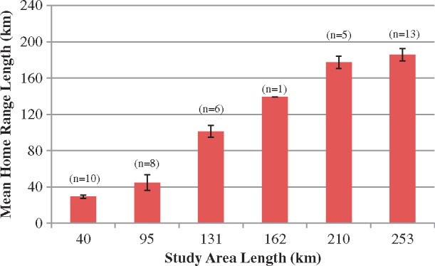
Mean 95% KDEs with increasing study area size for dolphins sighted ≥10 times. Error bars display the 95% confidence interval.

Figure 5.

Mean 50% KDEs with increasing study area size for dolphins sighted ≥10 times. Error bars display the 95% confidence interval.

The comparison of the SJR home range estimates calculated using the truncated and non-truncated midline indicated little difference between the two (Table 6). The 95% kernel density estimates (KDEs) from the full SJR midline ranged from 22.84 to 37.55 km, while for the truncated SJR midline the estimates ranged from 20.65 to 35.04 km. The 50% KDEs from the full midline ranged from 5.32 to 17.21 km, and from the truncated midline they ranged from 4.38 to 19.4 km.

Table 6.

Comparison of home range and core area estimates for individuals sighted ≥10 times in the St Johns River (SJR) using two versions of the midline

	95% HR (km)			50% CA (km)
ID code	Not truncated	Truncated	Difference	Not truncated	Truncated	Difference
NAIA	30.66	30.04	0.62	16.9	16.27	0.63
NASA	37.55	35.04	2.51	9.07	4.38	4.69
KIAW	34.73	30.98	3.75	9.70	12.20	−2.50
Q027	35.35	34.42	0.93	7.51	13.14	−5.63
PUKA	30.98	27.53	3.45	17.21	19.40	−2.19
Q142	22.84	20.65	2.19	5.32	5.01	0.31
LTUS	25.03	24.09	0.94	10.64	7.51	3.13
ZDCO	28.16	27.22	0.94	11.89	11.26	0.63
WIKD	35.98	34.73	1.25	12.83	9.70	3.13
Q080	25.35	24.41	0.94	7.19	5.94	1.25
Average	30.66	28.91	1.75	10.83	10.48	0.35

Notes: ‘Not truncated’ refers to the midline that extended all the way to the mouth of the SJR while ‘truncated’ refers to the midline that did not extend the full length of the SJR study area, but instead turned south to continue on to the intracoastal waterway (ICW) south through Duval County (DUV) study area.

Discussion

Maximum linear distance

As expected, the MLD increased as additional sightings from further study areas were added (Table 3). When the full 253 km study area was used, the average MLD (190 km) was higher than previously reported distances for estuarine dolphins (12–105 km; Balmer et al. 2008) and was much higher than mean linear distances reported for bottlenose dolphins in the Indian River Lagoon (22–54 km; Mazzoil et al. 2008). The largest MLD (215.96 km) was less than the 253 km combined study area, suggesting that our data may capture the true limits of these dolphins’ range (Table 3). In support of this, the data indicate that there may be a plateau in MLD with the inclusion of the last 2 study areas. These findings also demonstrate that these dolphins are not limited to one small estuarine area; some individuals traveled large distances across multiple study areas. However, one disadvantage of MLD analyses is that they do not incorporate weighting to account for differences in survey effort; they simply compute the distance from the 2 most extreme points. Although MLD provides valuable information on the full extent of the area traveled by an individual, it provides no information on space utilization.

Home range

Although the analyses conducted herein were for a subset of Northeast Florida’s estuarine dolphins, there was a clear pattern of increasing home range estimates as study area size increased (Figure 4). This is an indication that an analysis consisting of the 40 km SJR study area alone would not have properly estimated home range for these individuals given that the minimum home range was estimated at 116.40 km when all sites were included (Table 5). By combining all 253 km of study area, it appears that sufficient area has been covered since the largest home range was estimated at 217 km (Table 5); based on these values the percent coverage would be 86%. Home range size appears to reach an asymptote when all study areas are incorporated; the difference between home range estimates decreases as study area size increases (Figure 4). This pattern further supports the finding that the entire geographical range of these individuals has been reached. The findings from this study design are evidence that restricting analyses to a small study area may not give valid information regarding the range an animal actually covers, as many of the individuals within this study inhabited more than one research group’s study area. As this is one of only a few studies that have used the univariate kernel density method to date, and to our knowledge the only study for bottlenose dolphins, it is not yet possible to make direct comparisons between the estimates for this study region and other areas.

In contrast to the pattern observed with home range estimates, an increase in study area size did not correspond to an increase in core area size (Figure 5). There was no clear pattern between the estimated core areas and the size of the study areas, suggesting that even with a small study area, researchers may be able to accurately assess core area size. Although individuals travel large distances, they appear to concentrate their time in relatively small areas. Individuals may be able to utilize a relatively small area to meet their general resource needs, but movement to more distant areas may be required during certain circumstances (e.g., in response to reproductive status, unusual weather patterns, or anthropogenic disturbance events). A detailed analysis of habitat use within these expanded ranges would be highly informative. Finally, even though the analyses precluded the inclusion of a midline all the way to the mouth of the SJR, the data show that there is minimal difference in home range and core area estimates between the two methods (Table 6). Thus, both the MLD and KDE estimates calculated using the truncated midline are considered to have acceptable precision.

Individual variation in ranging patterns among animals in this study was very high. For example, there were individuals that were only sighted in the SJR and ML study areas as well as individuals that used the areas in-between. The patterns suggest that individuals may be traveling from the SJR to the southern study areas using different paths; some individuals appear to be using the ICW while others may not. The fact that individuals are not sighted in areas between the SJR and ML may indicate that these individuals are utilizing coastal areas rather than the ICW to move between regions. However, this gap of sightings between study areas may simply be due to random chance that those individuals were not in those areas on any of the survey days. Also, if those individuals are traveling through the intermediate areas quickly, they are more likely to be missed with infrequent surveys being conducted in those regions. These gaps in space affect the home range analyses in regards to how the utilization distributions are calculated, so it is important to discern whether the individuals are using these areas or not. Within the Northeast Florida region, 2 large estuarine areas have been documented providing year-round habitat for dolphins (Waring et al. 2016); this factor could potentially be driving the movement between the SJR and ML study areas. However, not all SJR dolphins are traveling the full distance between these estuaries.

When conducting home range studies, care must be taken beforehand to choose the appropriate method for analyses based on biological knowledge of each population and habitat. The univariate method used in this study improves upon prior studies by producing more usable information regarding the space traveled by individuals since it does not incorporate unusable area into KDEs. Many studies conduct bivariate home range analyses and remove the unusable area after the estimates are produced. This method biases the estimates compared with univariate analyses. Estuarine environments tend to be linear and narrow, so this method of analyzing home range may be useful for researchers working in similar environments. Additionally, for studies in which the number of sightings per individual are limited, it is beneficial to use univariate data since univariate estimates require fewer sightings when compared with bivariate estimates (Vokoun 2003).

Management

In addition to addressing the fundamental research question of the effects of study area size on home range estimates, there are clear management applications for this research. A population’s distribution is a key factor when making conservation management decisions, as it determines what areas need to be protected and to what extent. For example, the effectiveness of marine protected areas is likely limited by the quality of the distribution estimates used during their creation. In addition, knowledge of a population’s home range and core area can provide pertinent information regarding environmental pollutants and hazards when monitoring population health (Mazzoil et al. 2008).

Bottlenose dolphin populations in the United States are managed separately as individual stocks and therefore the range of each distinct population must be known. The National Oceanic and Atmospheric Administration currently considers the dolphins in the Jacksonville Estuarine System and the Indian River Lagoon Estuarine System to be 2 separate populations in their management plans (Waring et al. 2016). As displayed by the large MLDs and home range estimates reported here, individuals are not confined to the area currently defined as the Jacksonville Estuarine System. Thus, individuals from these different populations may not be geographically isolated from one another. If significant mixing occurs between these 2 populations, then management plans may need to be revised. NEFL DRC is currently analyzing rates of interchange between the Jacksonville Estuarine System and the Indian River Lagoon Estuarine System, in an effort to address this issue. In conclusion, this study demonstrates the need to expand survey areas in order to obtain more accurate home range estimates and thus illustrates the importance of conducting collaborative science.

The authors thank L. Gemma, T. Jablonski, and the many volunteers that assisted with this project. Drs. Julie Avery and Eric Johnson provided constructive comments which improved this manuscript. Research was conducted under National Marine Fisheries Service Level B Harassment Letter of Confirmations (No. 14157, 15631, 572-1869-02, and 16522) and UNF IACUC 10-013.

Funding

This project was funded by the Elizabeth Ordway Dunn Foundation (grant 11G2-15), the UNF Coastal Biology Flagship Program, the UNF Environmental Center, the San Marco Rotary Club, the SeaWorld Busch Gardens Conservation Fund, the Discover Florida’s Ocean license plate, and the Protect Wild Dolphins license plate. The Georgia Aquarium Conservation Field Station (GACFS) is an LLC under Georgia Aquarium Inc.

References

- Ballance LT, 1992. Habitat use patterns and ranges of the bottlenose dolphin in the Gulf of California, Mexico. Mar Mamm Sci 8:262–274. [Google Scholar]
- Balmer BC, Wells RS, Nowacek SM, Nowacek DP, Schwacke LH. et al. , 2008. Seasonal abundance and distribution patterns of common bottlenose dolphins Tursiops truncates near St. Joseph Bay, Florida, USA. J. Cetacean Res Manage 10:157–167. [Google Scholar]
- Balmer BC, Wells RS, Schwacke LH, Schwacke JH, Danielson B. et al. , 2014. Integrating multiple techniques to identify stock boundaries of common bottlenose dolphins Tursiops truncatus. Aquat Conserv Mar Freshw Ecosyst 24:511–521. [Google Scholar]
- Bas AA, Öztürk AA, Öztürk B, 2014. Selection of critical habitats for bottlenose dolphins Tursiops truncatus based on behavioral data, in relation to marine traffic in the Istanbul Strait, Turkey. Mar Mamm Sci31:979–997. [Google Scholar]
- Bejder L, Samuels A, Whitehead H, Gales N, Mann J. et al. , 2006. Decline in relative abundance of bottlenose dolphins exposed to long-term disturbance. Conserv Biol 20:1791–1798. [DOI] [PubMed] [Google Scholar]
- Borger L, Franconi N, de Michele G, Gantz A, Meschi F. et al. , 2006. Effects of sampling regime on the mean and variance of home range size estimates. J Anim Ecol 75:1393–1405. [DOI] [PubMed] [Google Scholar]
- Bowman AW, Azzalini A, 1997. Applied Smoothing Techniques for Data Analysis. Oxford: Clarendon Press. [Google Scholar]
- Burt WH, 1943. Territoriality and home range concepts as applied to mammals. J Mammal 24:346–352. [Google Scholar]
- Candido AT, Dos Santos ME, 2005. Analysis of movements and home ranges of bottlenose dolphins in the Sado estuary, Portugal, using a Geographical Information System (GIS). Abstract of 16th Biennial Conference on the Biology of Marine Mammals, San Diego, CA, USA.
- Connor RC, Wells RS, Mann J, Read AJ, 2000. The bottlenose dolphin: social relationships in a fission–fusion society In: Mann J, Connor RC, Tyack PL, Whitehead H, editors. Cetacean Societies: Field Studies of Dolphins and Whales. Chicago: University of Chicago Press, 91–126. [Google Scholar]
- Davis DE, 1953. Analysis of home range from recapture data. J Mammal 34:352–358. [Google Scholar]
- DeMort CL, 1991. Chapter 7: the St. Johns River system In: Livingston RJ, editor. The Rivers of Florida. Vol. 83 New York: Springer-Verlag, 97–120. [Google Scholar]
- Eisenberg JF, 1966. The social organization of mammals. Handb Zool 10:1–92. [Google Scholar]
- Folkens P, Reeves RR, Stewart BS, Clapham PJ, Powell JA, 2008. National Audubon Society Guide to Marine Mammals of the World. New York: Alfred A. Knopf. [Google Scholar]
- Fury CA, Harrison PL, 2008. Abundance, site fidelity and range patterns of Indo-Pacific bottlenose dolphins Tursiops aduncus in two Australian subtropical estuaries. Mar Freshw Res 59:1015–1027. [Google Scholar]
- Garland T, 1983. Scaling the ecological cost of transport to body mass in terrestrial mammals. Am Nat 121:571–587. [Google Scholar]
- Gibson QA, Howells EM, Lambert JD, Mazzoil MM, Richmond JP, 2013. The ranging patterns of female bottlenose dolphins with respect to reproductive status: testing the concept of nursery areas. J Exp Mar Biol Ecol 445:53–60. [Google Scholar]
- Gruber JA, 1981. Ecology of the Atlantic bottlenosed dolphin Tursiops truncatus in the Pass Cavallo Area of Madagorda Bay, Texas [M.S. thesis], [College Station (TX)]: Texas A&M University. 182.
- Gubbins C, 2002. Use of home ranges by resident bottlenose dolphins Tursiops truncatus in a South Carolina estuary. J Mammal 83:178–187. [Google Scholar]
- Hanby CL, 2005. Use of a Geographic Information System (GIS) to examine bottlenose dolphin community structure in southeastern North Carolina [M.S. thesis]. [Wilmington (NC)]: University of North Carolina.
- Hansteen TL, Andreassen HP, Ims RA, 1997. Effects of spatiotemporal scale on autocorrelation and home range estimators. J Wildl Manage 61:280–290. [Google Scholar]
- Harestad AS, Bunnell FL, 1979. Home range and body weight: a re-evaluation. Ecology 60:389–402. [Google Scholar]
- Hastie GD, Wilson B, Wilson LJ, Parsons KM, 2004. Functional mechanisms underlying cetacean distribution patterns: hotspots for bottlenose dolphins are linked to foraging. Mar Biol 144:397–403. [Google Scholar]
- Heithaus MR, Dill LM, 2002. Food availability and tiger shark predation risk influence bottlenose dolphin habitat use. Ecology 83:480–491. [Google Scholar]
- Henry C, Poulle ML, Roeder JJ, 2005. Effect of sex and female reproductive status on seasonal home range size and stability in rural red foxes Vulpes vulpes. Ecoscience 12:202–209. [Google Scholar]
- Ingram SN, Rogan E, 2002. Identifying critical areas and habitat preferences of bottlenose dolphins Tursiops truncatus. Mar Ecol Prog Ser 244:247–255. [Google Scholar]
- Kiszka J, Simon-Bouhet B, Gastebois C, Pusineri C, Ridoux V, 2012. Habitat partitioning and fine scale population structure among insular bottlenose dolphins Tursiops truncatus in a tropical lagoon. J Exp Mar Biol Ecol 416–417:176–184. [Google Scholar]
- Lindstedt SL, Miller BJ, Buskirk SW, 1986. Home range, time, and body size in mammals. Ecology 67:413–418. [Google Scholar]
- Litz JA, Garrison LP, Fieber LA, Martinez A, Contillo JP. et al. , 2007. Fine-scale spatial variation of persistent organic pollutants in bottlenose dolphins Tursiops truncatus in Biscayne Bay, Florida. Environ Sci Technol 41:7222–7228. [DOI] [PubMed] [Google Scholar]
- Lynn SK, Wursig B, 2002. Summer movement patterns of bottlenose dolphins in a Texas Bay. Gulf Mex Sci 20:25–37. [Google Scholar]
- Mann J, Connor RC, Barre LM, Heithaus MR, 2000. Female reproductive success in bottlenose dolphins (Tursiops sp.): life history, habitat, provisioning, and group-size effects. Behav Ecol 11:210–219. [Google Scholar]
- Martinez-Serrano I, Serrano A, Heckel G, Schramm Y, 2011. Distribution and home range of bottlenose dolphins Tursiops truncatus off Veracruz, Mexico. Cienc Mar 37:379–392. [Google Scholar]
- Mazzoil M, Reif JS, Youngbluth M, Murdoch ME, Bechdel SE. et al. , 2008. Home ranges of bottlenose dolphins Tursiops truncatus in the Indian River Lagoon, Florida: environmental correlates and implications for management strategies. EcoHealth 5:278–288. [DOI] [PubMed] [Google Scholar]
- Mazzoil M, McCulloch SD, Defran RH, Murdoch E, 2004. The use of digital photography and analysis for dorsal fin photo-identification of bottlenose dolphins. Aquat Mamm 30:209–219. [Google Scholar]
- McNab BK, 1963. Bioenergetics and the determination of home range size. Am Nat 97:133–140. [Google Scholar]
- Merriman MG, Markowitz TM, Harlin-Cognato AD, Stockin KA, 2009. Bottlenose dolphins Tursiops truncates abundance, site fidelity, and group dynamics in the Marlborough Sounds, New Zealand. Aquat Mamm 35:511–522. [Google Scholar]
- Moyer MA, McCown JW, Oli MK, 2007. Factors influencing home-range size of female Florida black bears. J Mammal 88:468–476. [Google Scholar]
- Parra GJ, 2006. Resource partitioning in sympatric delphinids: space use and habitat preferences of Australian snubfin and Indo-Pacific humpback dolphins. J Anim Ecol 75:862–874. [DOI] [PubMed] [Google Scholar]
- Pirotta E, Laesser BE, Hardaker A, Riddoch N, Marcous M. et al. , 2013. Dredging displaces bottlenose dolphins from an urbanized foraging patch. Mar Pollut Bull 74:396–402. [DOI] [PubMed] [Google Scholar]
- Rayment W, Dawson S, Slooten E, Bräger S, Fresne SD. et al. , 2009. Kernel density estimates of alongshore home range of Hector’s dolphins at Banks Peninsula, New Zealand. Mar Mamm Sci 25:537–556. [Google Scholar]
- Shane SH, 1987. The behavioral ecology of the bottlenose dolphin [Ph.D. thesis]. [Santa Cruz (CA)]: University of California.
- Sprogis KR, Raudino HC, Rankin R, 2015. Home range size of adult Indo-Pacific bottlenose dolphins Tursiops aduncus in a coastal and estuarine system is habitat and sex-specific. Mar Mamm Sci 32:287–308. [Google Scholar]
- Urian KW, Hofmann S, Wells RS, 2009. Fine-scale population structure of bottlenose dolphins Tursiops truncatus in Tampa Bay, Florida. Mar Mamm Sci 25:619–638. [Google Scholar]
- Urian KW, Hohn AA, Hansen LJ, 1999. Status of the photo-identification catalog of coastal bottlenose dolphins of the Western North Atlantic. Report of a Workshop of Catalog Contributions, NOAA Technical Memorandum NMFS-SEFSC-425, 22 pp. Available from: www.nmfs.gov.
- Vokoun JC, 2003. Kernel density estimates of linear home ranges for stream fishes: advantages and data requirements. N Am J Fish Manag 23:1020–1029. [Google Scholar]
- Waring GT, Josephson E, Maze-Foley K, 2016. U.S. Atlantic and Gulf of Mexico marine mammal stock assessments: 2015. NOAA Tech Memo NMFS-NE-238.
- Wells RS, 1991. The role of long-term study in understanding the social structure of a bottlenose dolphin community In: Pryor K, Norris KS, editors. Dolphin Societies: Discoveries and Puzzles. Berkeley: University of California Press, 199–225. [Google Scholar]
- Wells RS, Scott MD, Irvine AB, 1987. The social structure of free-ranging bottlenose dolphins In: Genoways HH, editor. Current Mammalogy. Vol. I New York: Plenum Press, 407–416. [Google Scholar]
- White GC, Garrot RA, 1990. Analysis of Wildlife Radio-Tracking Data. San Diego: Academic Press. [Google Scholar]
- Williams TM, Friedl WA, Fong ML, Yamada RM, Sedivy P. et al. , 1992. Travel at low energetic cost by swimming and wave-riding bottle-nosed dolphins. Nature 355:821–823. [DOI] [PubMed] [Google Scholar]
- Wilson B, Thompson PM, Hammond PS, 1997. Habitat use by bottlenose dolphins: seasonal distribution and stratified movement patterns in the Moray Firth, Scotland. J Appl Ecol 34:1365–1374. [Google Scholar]
- Zolman ES, 2002. Residence patterns of bottlenose dolphins Tursiops truncatus in the Stono River Estuary, Charleston County, South Carolina, U.S.A. Mar Mamm Sci 18:879–892. [Google Scholar]