Shale Gas Development and Drinking Water Quality

The extent of environmental externalities associated with shale gas development (SGD)is important for welfare considerations and, to date, remains uncertain (Mason, Muehlenbachs, and Olmstead 2015; Hausman and Kellogg 2015). This paper takes a first step to address this gap in the literature. Our study examines whether shale gas development systematically impacts public drinking water quality in Pennsylvania, an area that has been an important part of the recent shale gas boom. We create a novel dataset from several unique sources of data that allows us to relate SGD to public drinking water quality through a gas well's proximity to community water system (CWS) groundwater source intake areas.¹ We employ a difference-in-differences strategy that compares, for a given CWS, water quality after an increase in the number of drilled well pads to background levels of water quality in the geographic area as measured by the impact of more distant well pads. Our main estimate finds that drilling an additional well pad within 1 km of groundwater intake locations increases shale gas-related contaminants by 1.5–2.7 percent, on average. These results are striking considering that our data are based on water sampling measurements taken after municipal treatment, and suggest that the health impacts of SGD through water contamination remains an open question.

I. Data and Summary Statistics

Carnegie Museum of Natural History Pennsylvania Unconventional Natural Gas Wells Geodatabase provides a cleaned version of all drilling data from the PA Department of Environmental Protection (PADEP) as of 2015. These data allow us to identify the location of Marcellus shale gas wells, the dates of when well permits are issued, and the dates on which drilling began, known as “spud” dates. Since well activities often occur in waves, we group well bores within one acre of each other into “well pads” following Muehlenbachs, Spiller, and Timmins (2015), and then take the earliest recorded permit and spud date of a well pad as the relevant dates on which the associated activities of well pad preparation and drilling begin.

Drinking water measurements come from the PADEP Drinking Water Reporting System (DWRS). The DWRS provides sampling results as regulated by the Environmental Protection Agency Safe Drinking Water Act (SDWA) for all CWS from 2011 through 2015. These data also include related water sampling information such as the sample date, time-of-day, the contaminant sampled and its measured amount.

Next, we obtain data describing 5,049 groundwater intake locations as of 2015, which we build from the PADEP website. For each intake, the data include the exact location and the unique drinking water system identifier for which it is a source. Crucially, these intake locations allow us to link gas well activity to DWRS drinking water quality to produce our unique dataset.

To construct our estimation data, we first spatially link the intakes of groundwater-based CWS to all well pads within a large buffer, e.g., 10 km. Figure 1 provides the distribution of gas wells and groundwater intake wells in Pennsylvania. Based on this spatial relationship, we then associate a system's water quality sampling results to well pads that are near any of the system's groundwater intakes. Finally, we aggregate the total number of spudded well pads by the time a sample is taken across all well pads within various proximities to define gas well threats. Our main data, which is limited to chemicals that are likely related to SGD, results in 54,809 water samples that span 5 years beginning from 2011 for 424 community water systems, whose intakes lie within 10 km of at least one well pad. To account for any potential effects of weather fluctuations on water measurements, we control for the daily maximum temperature and precipitation around each groundwater intake location using data from Schlenker and Roberts (2009).

Figure 1. Distribution of Well Pads and Groundwater Sources.

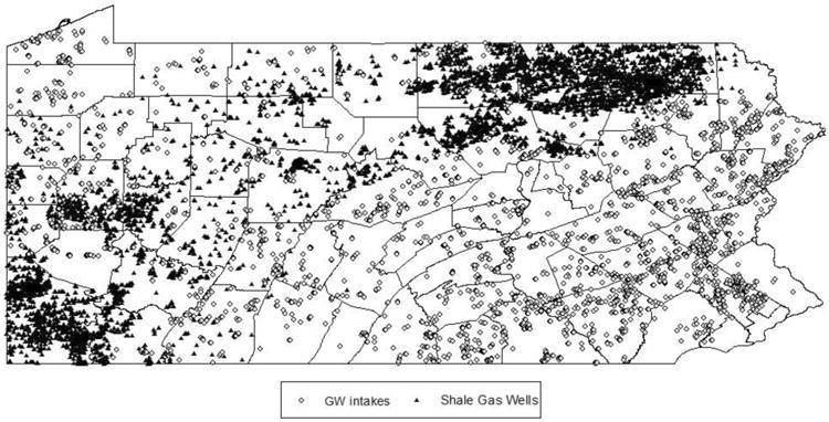
Table 1 provides summary statistics for the estimation sample. Water systems in our data serve an average population of 787 (s.d. 1,876). Compared to the largest public water systems in Pennsylvania, which can serve over 1.9 million people, the group of systems near Marcellus shale gas wells serves a small share of the population. As systems may source water from multiple locations, we observe that a CWS has an average of 2.9 intake locations (s.d. 2.4). Lastly, water samples have, on average, 0.02 to 0.45 well pads drilled within 0.5 to 2 km of their intakes.

Table 1. Summary Statistics.

	Mean	SD
CWS characteristics
Population served per CWS	787	1,876
Number of intakes per CWS	2.89	2.37
Observations	424
Water sampling characteristics
log(SCD water contaminant)	0.84	0.19
Well pads drilled within “d” km of water sample's intake
0.5 km	0.02	0.16
1 km	0.10	0.40
1.5 km	0.24	0.66
2 km	0.45	1.10
10 km	12.9	21.3
Observations	54,809

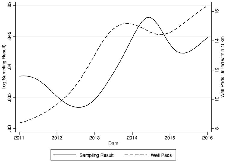
Figure 2 plots weighted averages of the number of drilled well pads and SGD-related water sampling results over time. This uses our main estimation sample, which includes water systems that have at least one well pad within 10 km of their groundwater intakes. Averages are smoothed using a gaussian kernel with a bandwidth of 177 days (set according to three times Silverman's Rule of Thumb). Although the magnitude of the increase in average water sampling results is modest, the relationship between the number of well pads and SGD chemical sampling measurements is compelling.

Figure 2. Water Sampling and Number of Drilled Well Pads over Time.

II. Empirical Strategy

We estimate the water quality impacts of well pad activities focusing on the set of contaminants that have been associated with SGD. We model the logarithm of water quality measurements, r_it, for a community water system j to depend on all K well pads within 10 km that have been spudded by the sampling date. We additionally distinguish well pads (indexed by k)within a smaller buffer (e.g., 1 km) of a sample i ( $d_{jk}^{<11}=1$) from those that are within 10 km but outside of 1 km ( $d_{jk}^{<10}=1$). We include sample-specific information (X_it) by controlling for the hour-of-day of when a sample was collected, the laboratory at which sampled results were measured, and the contaminant group to which a pollutant belongs.² The regression also controls for weather (e.g., precipitation and temperature), county-by-year fixed effects (ν_jt), quarter fixed effects (q_t), and a fixed effect for each CWS, cws_j. The following gives our baseline specification:

$$r_{it}={\beta }_1{\sum }_k^K{d}_{jk}^{<1}{w}_{kt}+{\beta }_2{\sum }_k^K{d}_{jk}^{<10}{w}_{kt}+X_{it}+v_{jt}+q_t+{\mathit{\text{cws}}}_j+{\epsilon }_{it},$$ (1)

where w_kt = 1 if well pad k has been spudded by time t. The parameter of interest, β₁, returns the impact of an additional well pad drilled by time t on the level of SGD-related contaminants measured, controlling for general water quality trends in the geographic area as captured by the drilling of more distant well pads, $\sum K^k{d}_{jk}^{<10}{w}_{kt}$.

Because elevation affects groundwater flow, we can additionally differentiate the water quality impacts of uphill well pads from those downhill. Gas well threats are defined to be “uphill” from a groundwater source if the lowest surface elevation of the well pad is higher than the surface elevation at the source intake location. We augment equation (1) by decomposing the total number of threats nearby into those uphill and downhill,

$${\sum }_k^K{d}_{jk}^{<1}={\sum }_k^K({\mathit{\text{up}}}_{jk}^{<1}+{\mathit{\text{down}}}_{jk}^{<1})$$ (2)

Recognizing that downhill well pad threats are less likely to impact water quality at intake wells, we would expect uphill threats to have stronger impacts on drinking water quality.

III. Results

Table 2, panel A shows our main regression results for drinking water quality as specified in equation (1). We present results using multiple “near” exposure buffers ranging from 0.5 km to 2 km. We find that an additional well pad within 0.5 km increases average SGD-related contaminant levels by a statistically significant 2.7 percent in column 1 of Table 2. Intuitively, when we allow the exposure buffer to increase, we find smaller effects on SGD contaminant levels for threats farther away; the average impact of an additional well pad within 1 km decreases to 1.5 percent in column 2. Well pad impacts for exposure buffers beyond 1 km (shown in columns 3 and 4) dissipate even more and are no longer statistically significant. Focusing on general water quality trends, as captured by well pads drilled within 10 km, we find that water quality seems to be stable and even slightly improving over this time period. Panel B explores any heterogeneity by elevation of the well pad. As before, impacts of well pads are limited to ones that are drilled within 1 km of intakes. While up- and downhill impacts are generally not statistically different from each other, it is reassuring that the magnitude of uphill threats are larger than those downhill. ³ These provide evidence that, unsurprisingly, it is the uphill threats that are disproportionately affecting drinking water quality

Table 2. Water Quality Impacts of Well Pad Spudding.

	d ≤ 0.5 km	d ≤ 1 km	d ≤ 1.5 km	d ≤ 2 km
Panel A. By distance to well pad
Pads in “d” km	0.0269 (0.0106)	0.0149 (0.00863)	0.000516 (0.00655)	0.00492 (0.00584)
Pads in 10 km	−0.000187 (0.000248)	−0.000313 (0.000287)	−0.000111 (0.000259)	−0.000366 (0.000319)
Observations	54,809	54,809	54,809	54,809
Panel B. By elevation to intake
Downhill pads in “d” km		0.00202 (0.0227)	−0.00643 (0.00895)	−0.000847 (0.00560)
Uphill pads in “d” km	0.0264 (0.0104)	0.0155 (0.00803)	0.00163 (0.00710)	0.00648 (0.00739)

Notes: Each column is a separate regression. Observations = 54,809 for each of the weight regressions reported. For panel B, pads up- and down-hill within 10 km are included but not shown. Robust standard errors in parentheses are clustered at the CWS level. The dependent variable is log(SGD chemicals).

IV. Conclusion

This paper estimates drinking water quality effects of SGD in Pennsylvania, and finds localized impacts for well pads drilled within 1 km of drinking water source intakes. A recent study finds that Pennsylvanians in counties with shale gas development spent $19 million on bottled water in 2010 due to perceived risks to drinking water (Wrenn, Klaiber, and Jaenicke 2016). Our results suggest that these perceived risks may in fact be justified. In assessing the costs of these impacts, however, one must simultaneously consider the share of the population that is exposed to these drinking water externalities: although 83 percent of the population in Pennsylvania sources drinking water from community water systems, only 14 percent are served by groundwater CWSs. While there are potentially large costs related to drinking water violations in terms of health (Currie et al. 2013) and avoidance behavior (Graff Zivin, Neidell, and Schlenker 2011; Wrenn, Klaiber, and Jaenicke 2016), the associated external costs of these well pad developments in Pennsylvania are likely to be small due to the size of the affected population. An important caveat is that exposure to SGD activity largely depends on the location of shale plays and is thus heterogeneous across regions. The advent of horizontal drilling has allowed SGD operations to proceed in densely populated urban areas, where drinking water source locations may be close by. As such, our estimates would imply large external costs from compromises to drinking water quality if applied to other regions of SGD activity.⁴ These results not only inform policymakers who set and enforce health-protective standards for the industry, but researchers who study the mechanisms of pollutant exposure to better understand how these operations affect health in their communities.

References

- Currie Janet, Zivin Joshua Graff, Meckel Katherine, Neidell Matthew, Schlenker Wolfram. Something in the Water: Contaminated Drinking Water and Infant Health. Canadian Journal of Economics. 2013;46(3):791–810. doi: 10.1111/caje.12039. [DOI] [PMC free article] [PubMed] [Google Scholar]
- Graff Zivin Joshua, Neidell Matthew, Schlenker Wolfram. Water Quality Violations and Avoidance Behavior: Evidence from Bottled Water Consumption. American Economic Review. 2011;101(3):448–53. [Google Scholar]
- Hausman Catherine, Kellogg Ryan. Welfare and Distributional Implications of Shale Gas. Brookings Papers on Economic Activity (Spring) 2015:71–125. [Google Scholar]
- Mason Charles F, Muehlenbachs Lucija A, Olmstead Sheila M. The Economics of Shale Gas Development. Resources for the Future Discussion Paper. 2015:14–42. [Google Scholar]
- Muehlenbachs Lucija, Spiller Elisheba, Timmins Christopher. The Housing Market Impacts of Shale Gas Development. American Economic Review. 2015;105(12):3633–59. [Google Scholar]
- Schlenker Wolfram, Roberts Michael J. Nonlinear Temperature Effects Indicate Severe Damages to US Crop Yields under Climate Change. Proceedings of the National Academy of Sciences. 2009;106(37):15594–98. doi: 10.1073/pnas.0906865106. [DOI] [PMC free article] [PubMed] [Google Scholar]
- Wrenn Douglas H, Allen Klaiber H, Jaenicke Edward C. Unconventional Shale Gas Development, Risk Perceptions, and Averting Behavior: Evidence from Bottled Water Purchases. Journal of the Association of Environmental and Resource Economists. 2016;3(4):779–817. [Google Scholar]