Compositional Proteomics: Effects of Spatial Constraints on Protein Quantification Utilizing Isobaric Tags

Abstract

Mass spectrometry (MS) has become an accessible tool for whole proteome quantitation with the ability to characterize protein expression across thousands of proteins within a single experiment. A subset of MS quantification methods (e.g., SILAC and label-free) monitor the relative intensity of intact peptides, where thousands of measurements can be made from a single mass spectrum. An alternative approach, isobaric labeling, enables precise quantification of multiple samples simultaneously through unique and sample specific mass reporter ions. Consequently, in a single scan, the quantitative signal comes from a limited number of spectral features (≤11). The signal observed for these features is constrained by automatic gain control, forcing codependence of concurrent signals. The study of constrained outcomes primarily belongs to the field of compositional data analysis. We show experimentally that isobaric tag proteomics data are inherently compositional and highlight the implications for data analysis and interpretation. We present a new statistical model and accompanying software that improves estimation accuracy and the ability to detect changes in protein abundance. Finally, we demonstrate a unique compositional effect on proteins with infinite changes. We conclude that many infinite changes will appear small and that the magnitude of these estimates is highly dependent on experimental design.

Introduction

The field of compositional data analysis was largely developed by the mathematical geoscience community with major contributions from Aitchison¹ and Egozcue.² Researchers interested in studying the geochemical compositions of rocks and sediment frequently converted raw measures of mineral abundance to proportions or ratios. The quintessential feature of compositional data is a constraint on the outcomes. Consequently, increases in one component necessarily affect the other components in order to satisfy the constraint. Consider a measurement with four equal parts. In an unconstrained scenario, doubling one part does not affect the absolute amount of the remaining three parts (Figure 1a); however, if the data are constrained, doubling one part will decrease the absolute amount observed in each component (Figure 1b).

Figure 1.

Isobaric tag proteomics data is inherently compositional. (A, B) The defining feature of compositional data is a constraint on the outcomes. These bar plots show the difference between doubling a component of unconstrained (A) versus constrained (B) data. In the unconstrained case, the measurements of each component are independent of one another so that doubling one quantity has no effect on the others. With constrained data, doubling the amount of one component necessarily decreases the magnitude of one or more other components. (C) Spectra from peptide AGLDNVDAESK. In the first run (top), only two channels were used, TMT126 and TMT128, at a ratio of 1:5, respectively. In the second run (bottom), these channels were kept the same but we added the peptide in a third channel, TMT130, at 10× of TMT128. We show that while the ratios of the values remain constant, the observed intensities of TMT126 and TMT128 were greatly reduced in the three-channel experiment. The intensity in channel 128 decreased from approximately 30 000 in the two-channel experiment to approximately 10 000 when a third TMT channel was added.

Quantitative mass spectrometry is inherently compositional because the population of ions that is measured for each spectrum is constrained. This constraint is necessary to ensure that gas phase ions respond to the electrical fields, while trapped within a mass spectrometer, in a predictable manner. The introduction of too many ions into a mass spectrometer can lead to space-charging effects that disturb ion isolation and/or mass analysis. Constraining the ion population number is actualized by automatic gain control (AGC), which attempts to allow a predictable number of ions into a mass spectrometer for a single injection.

The compositional nature of quantitative MS data has not been described, presumably because the effects are minimal in many types of MS experiments. For example, SILAC or label-free experiments quantify intact peptides from a spectrum that contains hundreds of features. In this situation, doubling the signal of one feature will decrease the signal for the remaining features a negligible amount. Conversely, the compositional nature of MS data has a much more profound effect when utilizing isobaric labels for quantitation, e.g., tandem mass tags (TMT),³ isobaric tags for relative and absolute quantitation (iTRAQ).⁴ This is because the spatial constraint is imposed on the isolated, prefragmented ion flow so that the signal is split among a small number of features (≤11).

In this article, we explore the effects of spatial constraints on the analysis and interpretation of isobaric tag proteomics experiments. We provide examples of comparisons that are nonsensical from a compositional perspective that would have been reasonable absent spatial constraints. We propose a statistical model for compositional proteomics and evaluate its performance in terms of accuracy, sensitivity, and specificity on two separate ground truth experiments.

We also show how compositional constraints can have different effects on experimental outcomes depending on the experimental design. Specifically, we show that infinite changes do not have to appear large and that changes in how samples are multiplexed can have a predictable effect on the estimates of infinite changes.

Experimental Procedures

Compositional Data Analysis

While the compositional aspect of mass spectrometry is theoretically explained by AGC constraints, it is another matter to directly observe the effects. To demonstrate the compositional nature of quantitative data resulting from isobaric tags a synthetic peptide, AGLDNVDAESK, was labeled with three quantitative channels of tandem mass tags (TMT-126, -128, and -130), and two samples were constructed, mixed at ratios of 1:5:0 and 1:5:50. They were then analyzed separately utilizing high-resolution MS.

The dependency between outcomes that we seek to show in this experiment greatly complicates data analysis. Even basic operations such as addition become inappropriate, as alterations to single components can violate the constraint. Fortunately, mathematical operations and probability distributions have been created for statistical analysis on a constrained sample space.^5,6 Commonly used distributions include the Dirichlet and Additive Log Normal.⁷ For all distributions, the standard approach for analyzing compositional data is to transform into an unconstrained space, perform an analysis, and transform back as needed.

The concept of transforming our data out of compositional space and then performing an analysis is the foundation of our modeling efforts. However, much more is required to account for the highly unbalanced and nested nature of the data. We create a model that utilizes the additive log-normal transformation (ALR), incorporates peptide level covariates to improve estimation, and utilizes partially pooled variance estimates⁸ to share information about the error structure across the whole data set.

Partially pooled variance estimators are especially useful for dealing with the unbalanced aspect of the data. In a model with no pooling, every protein fold change would have its own variance estimate. Unfortunately, for proteins with a small number of peptides, these estimates will not be very reliable. A potential solution to this problem is to use pooled variance so that a single experimental error is estimated and used for all proteins. While this is solves the problem of unreliable estimates in proteins with few peptides, it creates a new problem in that proteins with many peptides and little variation will now have an overestimated variance. A model with partially pooled variance components will yield estimates close to the completely pooled experimental error when only a few data points are observed. However, as the observations within a protein increase, the estimate will converge to the result with no pooling. Full model specifications and motivations are provided in Supporting Information Methods and Discussion S1.

The compositional transformation, peptide level covariate adjustments, and partially pooled variance estimation are all available in our R package, which contains precompiled Stan models to make use of efficient Bayesian simulation algorithms.⁹

Two-Proteome Ground Truth Experiments for Analyzing Accuracy and Detectability

To evaluate the performance of our compositional modeling, we used two separate two-proteome ground truth experiments. The first experiment contains a wide range of changes from yeast proteins mixed into a background of proteins extracted from mouse brain tissue. This experiment provides us with the opportunity to study small, large, and even infinite changes and allows us to explore quantitative extremes that may occur in a proteomics experiment. We will refer to this as the boundary case experiment. Details of the experimental design and procedure along with full data tables can be found in the Supporting Information. A second ground truth experiment (the common case experiment) targeted 2- and 3-fold changes by mixing yeast at defined ratios within a background of human proteins and was designed to closely mimic the proportion and scale of changes found in common biological experiments. The details of this experiment are shown in the Supporting Information. Each experiment was analyzed with both FT-MS2 and SPS-FTMS3 technologies^10,11 (we will often abbreviate these methods as MS2 and MS3, respectively).

Dual Multiplexed Viral Infection Experiment for Analyzing Infinite Changes

To explore the effect of spatial constraints on infinite fold changes, we reanalyzed samples from a time course in primary human fetal foreskin fibroblasts (HFFFs) infected with cytomegalovirus (HCMV), originally generated by Weekes et al.¹² In this experiment, we have duplicate uninfected samples as well as infected samples after 6, 12, 18, 24, 48, 72, and 96 h. We expect that the distribution of relative viral protein estimates from the uninfected sample to the 48 h time point will be different depending on what other time points are coanalyzed in the mass spectrometer. To this end, we reanalyzed aliquots from the original experiment as both a 10-plex and 2-plex containing only the untreated and 48 h time point. Details of the experimental procedure are given in Supporting Information Methods and Discussion S1.

Results and Discussion

Compositional Nature of Isobaric Tag Proteomics Data

It is important emphasize that isobaric tag proteomics data are compositional by their very nature. All types of data, when converted to proportions or ratios, demonstrate the properties of compositional data. However, with these data, the properties can be seen prior to any sort of mathematical manipulation. This was demonstrated by analyzing a synthetic peptide, AGLDNVDAESK, in two different multiplexing configurations (Figure 1C). Both runs 1 and 2 exhibited a 1:5 ratio between channels 126 and 128; however, when channel 130 was added in run 2, the intensity of channel 128 was dramatically reduced from ∼30 000 to ∼10 000. This is the essence of compositional data: adding to one channel necessarily reduces the signal in at least one other channel. This dependence makes direct comparison of TMT reporter ion intensities across separate MS2 spectra unreliable.

Predictably, the effect shown in Figure 1C will only be seen for scans where the AGC limit has been reached. In the absence of the constraint on ion sampling, more ions can be collected from a new channel without necessarily decreasing the signal from the other channels. It should be noted that many factors might contribute to a change in the signal-to-noise ratio for a given reporter ion. However, there is nothing special about the peptide shown in Figure 1C other than the fact that the AGC limit was reached. The same behavior will be observed whenever a lack of space necessitates a decrease in ion injection time.

Not all scans will hit the AGC target, but ignoring the measurements that do is not a viable option. In our boundary case FT-MS2 experiment, the AGC limit was reached in 92% of the scans. In the SPS-FTMS3 version of the experiment, the limit was hit over 99% of the time. This difference in percentages could be caused by the expanded isolation window created by synchronous precursor selection. However, many variables might affect the frequency of hitting the AGC target, especially the complexity of peptide mixtures and the actual abundance of a specific protein. In any case, the result is a data set that is only partly compositional by nature.

To make matters more confusing, we cannot ever directly “see” the constraint. This is because the constraint is imposed on the isolated prefragmented ion flow. Variations in fragmentation efficiency guarantee that the number of ions that contribute to the reporter ion signals will not directly match up to the number of ions that were constrained in the C-Trap. Furthermore, the number of species of ions in the MS2/MS3 scan (including a large number of fragment ions) is not reflective of the number of ion species that was initially constrained (<11). In all cases, whether compositional by nature or just by convenience, a compositional data analysis will be appropriate since analyzing the proportions is sensible even when it is not necessary.

Some of the consequences of compositional constraints are obvious, while others are very subtle. Among the obvious effects are complications that arise when comparing signals from different plexes. In compositional data, only the set of proportions that define the composition are pertinent. When comparing different plexes, the signal intensities might represent proportions from different wholes. For example, in Figure 1c, the average of the signals from channel 128, across plexes, is not a meaningful quantity. Interpreting a lower signal in run 2 as evidence that less of the peptide was present would be a severe mistake.

In the absence of the spatial constraint, we could assume changes in signal intensity across plexes to be a function of ion injection time. Accordingly, one might “normalize” the peptide signals from each plex by the total signal intensities across all channels. However, such strategies fail to account for the compositional aspect. If the designs in each plex are not equivalent, then increases in some channels will result in decreases in others even when the total signals are equal. Accordingly, a drop in signal across plexes still does not necessarily imply a drop in abundance. Our modeling efforts, based on principles of compositional data analysis, avoid these problems by analyzing only the relevant ratio information from each scan. Incorporating other peptide level information is handled by adding covariates to our modeling.

For example, both isolation specificity (IS) (Figure 2B) and summed signal-to-noise (SSN) (Figure 2C) are peptide level statistics that have an observable effect on the MS2 intensity ratios shown in Figure 2D,E. The scatterplot shows that large ratios tend to be compressed as both isolation specificity and summed signal-to-noise decrease. In theory, we should be able to exploit relationships between intensity ratios and known peptide level information to our advantage.

Figure 2.

Relationship between two peptide level covariates and ratio compression. (A) Diagram explaining the ratios and experimental design for the data plotted in (D) and (E). We highlight here 1-, 4-, and 100-fold changes with MS2 quantification from the boundary case experiment. This is a two species interference model with abundance of mouse proteins kept constant across channels and yeast proteins diluted at known ratios. (B) Isolation specificity is a statistic that can be calculated for each peptide spectral match. With current technologies, the ability to accurately measure mass exceeds our ability to isolate those masses. Consequently, the isolation window used to select a specific mass for MS2 analysis will usually contain more than a single peak. The isolation specificity statistic is an attempt to quantify the proportion of signal belonging to the peak that we intended to target. (C) Another peptide level statistic of interest is the total sum of signal-to-noise ratios. In the theory of compositional data, the total amount of signal collected should be irrelevant given all of the ratio information. However, in proteomics experiments, the total amount of signal may have an effect on the precision and accuracy of the ratios. (D, E) Scatterplots demonstrating the relationship between log ratio peptide intensities and two peptide level statistics, isolation specificity (IS) (D) and summed signal-to-noise (SSN) (E). Both relationships show trends that mimic the ratio compression that we expect to see from interfering ions. This suggests that either IS or SSN could be used as covariates in a regression to somewhat mitigate the effects of compression. However, the slopes of the lines depend on the true change, greatly complicating modeling efforts.

An example of how to perform such an analysis is shown in Figure 3. The details of the analysis are given in Supporting Information Methods and Discussion S1. The key aspect is that we first conceptualize each scan as a composition (set of proportions). The proper mathematical space for compositions is the simplex (triangle of arbitrary dimensions), which is graphically represented with a ternary diagram. We then transform using the additive log ratio (ALR) transformation⁵ and fit regression lines in real space. At this point, we could draw conclusions about the log ratios or convert back to the simplex as needed.

Figure 3.

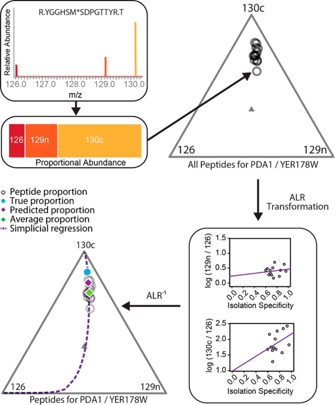
Workflow for a compositional data analysis. For a specific peptide spectral match, we first convert reporter ion intensities to proportions and plot them in a ternary diagram. This plot contains all of the peptide measurements that belong to protein YER178W, found in the MS2 boundary case experiment (other tags are excluded for graphical simplicity). The appropriate geometric space for constrained data is a simplex (triangle of arbitrary dimension), which motivates the use of ternary diagrams. Each vertex represents one component, and the inverse distance from a vertex to a point reflects the proportion of the composition belonging to that vertex. The additive log ratio (ALR) transformation is applied to each set of proportions, putting the data into the usual Cartesian geometric space. Linear regressions between the log ratios and isolation specificity (IS) are fit for each channel ratio. The inverse additive log ratio transformation is then applied to these results to create one simplicial regression. This regression line allows us to project what the protein composition would have been if the isolation specificity was equal to 1 (purple diamond). This value is roughly halfway between an estimate obtained by just averaging each peptide level proportion (green diamond) and the true protein level proportion (blue dot). Notice that in this plot IS closely mimics the effect of interference-induced compression, as values with lower IS are closer to unity (the center of the triangle).

In this ternary diagram, each point represents a three-part composition with components labeled on the vertices. For a given point, the proportion of an individual component is determined by the shortest distance from the point to the side of the triangle opposite the component’s vertex. This plot graphically demonstrates the relative and constrained nature of the data. All points in the simplex (triangle of arbitrary dimension) must sum to 1, and increases in any one component necessitate decreases in at least one other.

Converting back to the simplex and creating one simplicial regression line reveals the effect of IS in the compositional space. Interestingly, the line closely mimics the effect of MS2 compression as lower values of IS bring the composition closer to unity and predicted values when IS = 1 are brought closer to the true proportions.

Two-Proteome Ground Truth Experiments

We set out to create data with a wide range of known true fold changes. To this end, we used two species models where background proteins remained unchanged while proportions of yeast proteins varied across channels (Figure 4A,D).

Figure 4.

Improved modeling of the data enhances the accuracy and detectability of protein fold changes. (A, D) Design of two gold standard dilution experiments. In (A), we show the general setup for the boundary case experiment. A two proteome mixture was analyzed that supplemented a constant amount of mouse background (gray) with varying amounts of yeast protein (green). The ratios were selected to enable an analysis that pushes the boundaries of the type of changes seen in biological experiments, including small, large (100-fold), and infinite changes. In (D), we describe the common case experiment, which was designed to resemble typical biological experiments. Once again, yeast was varied using dilutions mixed into a human background. However, this time the changes were only 2- and 3-fold and the design contains multiple replicates. (B, E) In each dilution experiment, we compared estimates for the log₂ fold changes of yeast proteins from four different methods against the true values. CompMS2 and CompMS3 represent the results from fitting the compositional models to MS2 and MS3 data, respectively. These box plots show the distribution of the absolute deviation from true changes for each method in the (B) boundary case and (E) common case experiments. (C, F) Receiver operating characteristic (ROC) plots of each dilution experiment. These ROC plots show the ability to detect 2-fold changed yeast proteins. The area under each curve is the probability that a true signal would have a higher predictive value than a false signal.

Performance of our compositional models was evaluated in terms of accuracy, sensitivity, and specificity. Since we know the true log₂ fold changes from our ground truth experiments, we can evaluate accuracy as the absolute deviation from the true results. As expected, the MS3 data were inherently more accurate than the MS2 data in both data sets (Figure 4B,E). In each experiment, the compositional modeling of MS2 data, using SSN, improved the accuracy of our estimates, but we were never able to match the accuracy of the MS3 methods.

The compositional modeling had little effect on the accuracy of MS3 experiments. This is expected because all of the methods applied to MS3 data yield estimates of protein log ratios that are similar to the average of observed peptide log ratios within the protein; i.e., in all MS3 models, the expected value of a peptide log ratio is the parameter that represents the protein log ratio. Consequently, the methods all yield very similar point estimates. However, the MS2 model does something a bit different. In the MS2 model, we estimate a parameter that determines the relationship between peptide ratios and SSN. Consequently, the parameter for the protein log ratio is defined as the expected value of the peptide log ratios when SSN is at the 99th percentile. So, rather than taking an average of observed peptide log ratios, we are actually targeting a prediction of what the peptide ratios would have been if the summed-signal-to-noise had been higher.

Regarding the ability to detect changes, we evaluate performance in terms of both sensitivity (the probability of detecting a change when it is real) and specificity (the probability of ignoring signals that should be ignored). These two aspects of signal detection must be evaluated together. Perfect sensitivity can always be obtained by simply calling everything “significant”. Receiver operating characteristics (ROCs) put both aspects into one plot. Figure 4C,F shows the ROC curves for 2-fold changes (plots for all of the other magnitudes are shown in Figures S2–S4). In the boundary case experiment, many proteins were quantified from only a single peptide ratio (the common case experiment always has replicates). For these cases, when using an ANOVA, standard errors and p-values cannot be generated (this is not a problem for the compositional model). To avoid making unfair comparisons, we took two approaches to generating ROC plots: one where we remove proteins with only a single observation and another where we use all proteins but assign a p-value of 1 in cases where they cannot be computed. From a signal detection framework, the latter might be preferable as these are observed signals that will never be detected. ROC plots generated from all available proteins are presented in Figures S2–S4, and plots based on proteins with two or more peptides are shown in the main text. Across all plots, clear methodological advantages are demonstrated, with compositional MS3 exhibiting the greatest ability to detect 2-fold changes in both experiments.

The effect of our modeling on the boundary case data (Figure 4C) was profound, showing a clear ordering with better detection with MS3 than MS2 data and better performance in both technologies with compositional modeling. Interestingly, the modeling was able to make signal detection on the less precise MS2 data better than what was achieved with an ANOVA on the MS3 data. The effect was less dramatic in the common case data (Figure 4F) as the replicates improve signal detection across all approaches. Nonetheless, the compositional model still provides the greatest signal detection as can be more clearly seen in the inset image magnifying the upper left corner of the plot. The rank ordering of methodologies is the same in both experiments, but it is important to note that the ROC plots characterize signal detection performance on a per signal basis.

An important element that cannot be assessed by ROC plots alone is the number of proteins with altered abundance that were detected by each method. These numbers are not very meaningful in the boundary case data set, where they primarily describe the number of dilution combinations, but in the common case data, they reflect what a researcher might expect to find in a real experiment. At a 1% false positive rate, using a standard t-test methodology, we were able to detect 1281 and 1188 2-fold changes with MS2 and MS3 data, respectively. The greater numbers for MS2, in spite of poorer performance in the ROC curve, is expected as MS2 scans require less instrument time than MS3, allowing more overall data to be collected. Impressively, the improved detection of quantitative differences enabled by the compositional model increases the number of true positives to 1754 and 1301. Per signal, the compositional modeling of MS3 data gave the best performance, but the depth of discovery obtained with compositional MS2 (35% more true positives than compositional MS3) provides a considerable advantage. Similar results can be seen for the 3-fold changes in Figure S5A.

It should be noted that the importance of methodology diminished as the magnitude of true changes increased (all methods perform well while detecting fold changes of 100). However, a surprising and notable exception is shown in Figure 5A, where the ROC plots for infinite changes show substantial differences between methodologies. The modeling benefit seen here is similar to what we observed for relatively small changes. This is explained by the fact that infinite changes frequently appeared very small in the boundary case experiment (Figure 5B). As such, the type of model used in this experiment had a large impact on our ability to detect infinite changes. Methodologies that enhance our ability to detect small changes also enhance our ability to detect infinite changes. This surprising result is further explored in the viral time course experiment.

Figure 5.

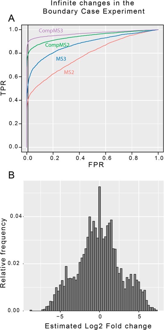
Infinite changes can appear small. (A) Receiver operating characteristic (ROC) plots for infinite changes in the boundary case experiment. In this plot, proteins with <2 observed peptides were removed since the ANOVA method cannot generate p-values with only a single data point. An alternative is to give these proteins a p-value of 1, since they were not detected, and compare signal detection on the entire data set (Figure S4D). (B) Histogram of the estimates of the log₂ fold changes for proteins, which we know are truly infinite, from the boundary case experiment. This shows that, contrary to typical expectations, infinite changes in TMT experiments can appear small.

Dual Multiplexed Viral Infection Experiment for Analyzing Infinite Changes

The compositional aspect of isobaric tag proteomics data has a special effect on infinite changes. We work with signal-to-noise measurements, which cannot be less than 1, so even if no ions are present in a given sample, we still observe some measurement near the noise. Conceptually, for a two-channel TMT experiment where one channel is empty, the mass spectrometer will continually sample from the present channel until the AGC is reached, resulting in a very large relative measurement. However, more complicated designs could alter this behavior.

Consider again the plot in Figure 1C. Adding a third channel greatly reduced the number of ions that could be collected from the first two channels. However, the compositional ion reduction may have a different impact on empty channels. Consequently, the relative measurement from an empty channel to one that is present might change in magnitude depending on the amount of ions from other channels.

Since spatial constraints reduce the number of ions collected in a scan but have no effect on the noise, we hypothesized that the distribution of infinite changes would be dependent on experimental design. To test this, we considered a time course experiment where a human fibroblast cell line is infected with cytomegalovirus. The time course samples were split up and multiplexed once with all 10 samples and separately with only 2 channels. We expected that constrained ion sampling in the 10-plex would result in lower true signals relative to the 2-plex. Consequently, we predicted that the infinite changes would appear larger in the 2-plex than the 10-plex. The distributions of average log ratios (Figure 6B) are consistent with this prediction.

Figure 6.

Space constraints combine with experimental design to predictably alter the appearance of infinite changes. (A) Workflow for our time course experiment. After adding TMT to each peptide digest, we multiplexed the samples as both a 2- and 10-plex and analyzed each separately in the mass spectrometer. (B) In these density plots, we show the distribution of the average log₂ peptide ratio, for each protein, from the untreated sample to the sample 48 h after infection. The two curves represent the distribution of changes when we multiplex all 10 samples in the time course (red) versus multiplexing only the two samples of interest (blue). The distribution of human proteins fold changes is basically identical in both designs (top). However, the viral proteins (infinite changes) are shifted (bottom). (C) Two example proteins are highlighted, one human (DDA1) and one viral (UL86). These plots show estimated log₂ fold changes between the untreated and 48 h time points. The colored boxes represent 80% credible intervals, whereas the black tails show 95% credible intervals. In both cases, the intervals were generated with our Bayesian compositional model. (D) ROC plots for two statistical methodologies in each of the multiplex designs. These ROC plots show the ability to detect infinite fold changes from viral proteins (true positives) versus human proteins (true negatives), most of which should be unchanged.

As expected, the distribution of human protein estimates remains virtually unchanged between experimental designs. However, the viral proteins are clearly affected by design, with the median estimate shifting by 0.78 on the log₂ scale (Figure 6B). In these density plots, we show the distribution of the average log₂ peptide ratio, for each protein, from the untreated sample to the sample 48 h after infection. We show the distribution of average ratios as opposed to model-based estimates to emphasize that this shift has nothing to do with advanced statistical modeling. The two curves represent the distribution of changes when we multiplex all 10 samples in the time course versus multiplexing only the two samples of interest. The distribution of human protein fold changes is basically identical in both designs (top). However, the viral proteins (infinite changes) are shifted (bottom).

Two example proteins are highlighted (Figure 6C), one human (DDA1) and one viral (UL86). DDA1, which associates with the Cullin-RING ligase 4 complex,¹³ had log₂ fold change estimates of 2.84 and 2.59 in the 10- and 2-plex, respectively. Looking at an infinite change such as for UL86, the major capsid protein in HCMV, the average log₂ fold change estimate shifts from 2.36 (∼5-fold) in the 10-plex up to 3.27 (nearly 10-fold) in the 2-plex.

These plots show estimated log₂ fold changes between the untreated and 48 h time points. The colored boxes represent 80% credible intervals, whereas the black tails show 95% credible intervals. Notice that while the estimated 10-plex fold change for DDA1 is completely contained in the 95% interval from the 2-plex, the intervals for the viral protein show complete separation. In the full 10-plex, ions from the 48 h time point have to compete with ions from the rest of the samples. This decreases the magnitude of all real signals in such a way that the proportions remain correct. However, no corresponding reduction occurs in the truly empty channels. This implies that  compositional constraints do not necessarily affect interfering ions in the same way as target ion populations. Consequently, infinite fold changes in two-channel experiments can appear larger than they would in more complicated designs.

Consistent with results from both the boundary case and common case experiments, we once again see improved signal detection capabilities when utilizing our compositional model. ROC plots for two statistical methodologies in each of the multiplexing designs show the ability to detect infinite fold changes from viral proteins (true positives) versus human proteins (true negatives), most of which should be unchanged (Figure 6D). In addition to this computational improvement we also see a substantial increase in detection ability as a consequence of experimental design. This is expected since infinite changes in the 2-plex experiment appear larger than they do in the 10-plex. Once again, proteins with <2 peptides were removed for the creation of this plot. The corresponding plot for all proteins is provided in the Supporting Information (Figure S5B).

Conclusions

We have demonstrated theoretically and experimentally that isobaric tag proteomics data are inherently compositional. This statement has profound implications for the analysis and interpretation of experiments. Comparisons that would have otherwise been sensible are no longer valid when considering the compositional aspect, and any interpretation of the data that relies on notions of absolute abundance are bound to be misguided. However, the lessons are not merely cautionary.

Statistical models based on principles of compositional data analysis can greatly improve the accuracy and detectability of small and infinite fold changes. In terms of sensitivity and specificity, our modeling was able to improve the detectability of 2-fold changes in MS2 data enough to outperform standard MS3 methods. On the basis of these results, we strongly recommend that both MS2 and MS3 data should be analyzed with our compositional models. Regarding the strengths of the underlying technologies, researchers who are primarily interested in the number of changed proteins discovered, at equivalent false positive rates, should use FT-MS2 technologies along with compositional modeling. For those who need either improved accuracy or the best ability to detect a change, on a per signal basis, SPS-FTMS3 with compositional modeling provides the best results.

The modeling gains are greatest for small changes, which may not be of great interest to some researchers. However, understanding the compositional nature of these experiments also led us to predict a previously unexplored behavior of mass spectrometry. When spatial constraints limit the signal from a target ion, the constraints do not necessarily have the same effect on the amount of interference. Consequently, the observed magnitude of infinite changes is a function of experimental design. This lesson is important for two reasons. One, infinite changes can appear small, which should be of substantial importance to researchers interested in gene activation/deactivation. Two, the methodological advantages demonstrated with our modeling efforts apply to infinite as well as small changes.

While the gains in accuracy and signal detection are important, the primary reason to treat isobaric tag data as compositional is not derived from these benefits. In our view, models should be designed to provide the most faithful representation of the data generating process possible. No other model properly accounts for the dependencies created by the spatial constraint, and any framework that does so properly would be compositional by definition. We have done our best to explore the benefits of accounting for the constraint and the dangers of ignoring this aspect. However, our imaginations are limited, and the consequences of compositional proteomics very likely exceed what we have here presented.

Supporting Information Available

The Supporting Information is available free of charge on the ACS Publications website at DOI: 10.1021/acs.jproteome.7b00699.

• Methods and Discussion S1; Software S1: directions for installing and using the compMS R package; Figure S1: assessing the convergence of a Stan model; Figure S2: ROC plots from the boundary case experiment for small fold changes; Figure S3: ROC plots from the boundary case experiment for fold changes of 4, 8, and 16; Figure S4: ROC plots from the boundary case experiment for large and infinite fold changes; Figure S5: ROC plots for 3-fold changes from the common case experiment and infinite changes from the time course experiment (PDF)

• Table S1: peptide level data from the MS2 boundary case experiment; Table S2: protein level posterior means and standard deviations from the MS2 boundary case experiment; Table S3: peptide level data from the MS3 boundary case experiment; Table S4: protein level posterior means and standard deviations from the MS3 boundary case experiment; Table S5: protein level posterior means and standard deviations from the MS2 common case experiment; Table S6: protein level posterior means and standard deviations from the MS3 common case experiment; Table S7: peptide level data from the 2-plex time course experiment; Table S8: protein level posterior means and standard deviations from the 2-plex time course experiment; Table S9: peptide level data from the 10-plex time course experiment; Table S10: protein level posterior means and standard deviations from the 10-plex time course experiment (XLSX)

The authors declare no competing financial interest.

References

- Aitchison J.The Statistical Analysis of Compositional Data; Chapman and Hall, 1986. [Google Scholar]
- Egozcue J. J.; Pawlowsky-Glahn V.; Mateu-Figueras G.; Barceló-Vidal C. Isometric Logratio Transformations for Compositional Data Analysis. Math. Geol. 2003, 35 (3), 279–300. 10.1023/A:1023818214614. [DOI] [Google Scholar]
- Thompson A.; Schäfer J.; Kuhn K.; Kienle S.; Schwarz J.; Schmidt G.; Neumann T.; Hamon C. Tandem Mass Tags: A Novel Quantification Strategy for Comparative Analysis of Complex Protein Mixtures by MS/MS. Anal. Chem. 2003, 75 (8), 1895–1904. 10.1021/ac0262560. [DOI] [PubMed] [Google Scholar]
- Ross P. L.; Huang Y. N.; Marchese J. N.; Williamson B.; Parker K.; Hattan S.; Khainovski N.; Pillai S.; Dey S.; Daniels S.; et al. Multiplexed Protein Quantitation in Saccharomyces Cerevisiae Using Amine-Reactive Isobaric Tagging Reagents. Mol. Cell. Proteomics 2004, 3 (12), 1154–1169. 10.1074/mcp.M400129-MCP200. [DOI] [PubMed] [Google Scholar]
- Aitchison J. The Statistical Analysis of Compositional Data. J. R. Stat. Soc. Ser. B. Methodol. 1982, 44 (2), 139–177. [Google Scholar]
- Pawlowsky-Glahn V.; Egozcue J. J. Geometric Approach to Statistical Analysis on the Simplex. Stoch. Environ. Res. Risk Assess. 2001, 15 (5), 384–398. 10.1007/s004770100077. [DOI] [Google Scholar]
- Pawlowsky-Glahn V.; Buccianti A.. Compositional Data Analysis: Theory and Applications; Wiley, 2011. [Google Scholar]
- Gelman A.; Hill J.. Data Analysis Using Regression and Multilevel/Hierarchical Models; Cambridge University Press, 2006; pp 251–275. [Google Scholar]
- Carpenter B.; Gelman A.; Hoffman M. D.; Lee D.; Goodrich B.; Betancourt M.; Brubaker M.; Guo J.; Li P.; Riddell A. Stan : A Probabilistic Programming Language. J. Stat. Softw. 2017, 76 (1), 1–32. 10.18637/jss.v076.i01. [DOI] [PMC free article] [PubMed] [Google Scholar]
- Ting L.; Rad R.; Gygi S. P.; Haas W. MS3 Eliminates Ratio Distortion in Isobaric Multiplexed Quantitative Proteomics. TL - 8. Nat. Methods 2011, 8 (11), 937–940. 10.1038/nmeth.1714. [DOI] [PMC free article] [PubMed] [Google Scholar]
- McAlister G. C.; Nusinow D. P.; Jedrychowski M. P.; Wühr M.; Huttlin E. L.; Erickson B. K.; Rad R.; Haas W.; Gygi S. P. MultiNotch MS3 Enables Accurate, Sensitive, and Multiplexed Detection of Differential Expression across Cancer Cell Line Proteomes. Anal. Chem. 2014, 86 (14), 7150–7158. 10.1021/ac502040v. [DOI] [PMC free article] [PubMed] [Google Scholar]
- Weekes M. P.; Tomasec P.; Huttlin E. L.; Fielding C. A.; Nusinow D.; Stanton R. J.; Wang E. C. Y.; Aicheler R.; Murrell I.; Wilkinson G. W. G.; et al. Quantitative Temporal Viromics: An Approach to Investigate Host-Pathogen Interaction. Cell 2014, 157 (6), 1460–1472. 10.1016/j.cell.2014.04.028. [DOI] [PMC free article] [PubMed] [Google Scholar]
- Gao S.; Geng C.; Song T.; Lin X.; Liu J.; Cai Z.; Cang Y. Activation of c-Abl Kinase Potentiates the Anti-Myeloma Drug Lenalidomide by Promoting DDA1 Protein Recruitment to the CRL4 Ubiquitin Ligase. J. Biol. Chem. 2017, 292 (9), 3683–3691. 10.1074/jbc.M116.761551. [DOI] [PMC free article] [PubMed] [Google Scholar]
Associated Data
This section collects any data citations, data availability statements, or supplementary materials included in this article.