Low Rank Approximation Methods for MR Fingerprinting with Large Scale Dictionaries

Abstract

Purpose

This work proposes new low rank approximation approaches with significant memory savings for large scale MR fingerprinting (MRF) problems.

Theory and Methods

We introduce a compressed MRF with randomized SVD method to significantly reduce the memory requirement for calculating a low rank approximation of large sized MRF dictionaries. We further relax this requirement by exploiting the structures of MRF dictionaries in the randomized SVD space and fitting them to low-degree polynomials to generate high resolution MRF parameter maps. In vivo 1.5 and 3 Tesla brain scan data are used to validate the approaches.

Results

T₁, T₂ and off-resonance maps are in good agreement with that of the standard MRF approach. Moreover, the memory savings is up to 1000 times for the MRF-FISP sequence and more than 15 times for the MRF-bSSFP sequence.

Conclusion

The proposed compressed MRF with randomized SVD and dictionary fitting methods are memory efficient low rank approximation methods, which can benefit the usage of MRF in clinical settings. They also have great potentials in large scale MRF problems, such as problems considering multi-component MRF parameters or high resolution in the parameter space.

Introduction

Recently, Ma et al. have developed a new quantitative magnetic resonance imaging technique, named Magnetic Resonance Fingerprinting (MRF) (1). Unlike conventional qualitative MRI, it uses variable acquisition parameters to gather tissue information based on specific signal evolutions within each voxel. After the signal evolutions are collected and recorded, a pattern matching algorithm is used to identify different tissue type parameters against a pre-calculated dictionary using the Bloch equation simulations with different combinations of parameters of interest, such as T₁, T₂, and off-resonance. This novel approach has drawn great attention from the magnetic resonance imaging community for both technical developments and clinical applications (2–12).

One of the challenges this approach faces though is the large amounts of data it generates, especially when fine MRF dictionaries are needed or multiple components, e.g. chemical exchange effects (13) or additional fields (14, 15) are taken into account. The number of elements in MRF dictionaries can easily reach billions in these cases, making storing, loading, and processing MRF dictionaries extremely difficult even when using modern computers.

The MRF dictionaries generated, however, are highly redundant. Thanks to this property, a low rank matrix approximation can reduce the size of MRF dictionaries significantly. For example, McGivney, et al. (16) have recently shown that the pattern matching step in MRF can be sped up by a factor of 40 for the MRF-FISP dictionary (17) and a factor of 5 for the MRF-bSSFP dictionary (18), by employing the singular value decomposition (SVD) to compress the time frame domain of the MRF dictionaries. However, the major contributor to the size of an MRF dictionary is the tissue property dimension, which is typically much larger than the time frame dimension. This makes the SVD approach infeasible if high resolution or large multi-dimensional analyses need to be taken into account. To compute the SVD, the dictionary needs to be generated and loaded into the computer memory in the first place. Moreover, note that for a matrix of size m × n, (assuming m ≤ n), the computational complexity of calculating the SVD of the matrix is O(m²n) floating-point operations (flops) (19). Therefore, even if the dictionary could be loaded into the memory, it is too expensive to perform the SVD for large sized dictionaries.

Cauley, et al. (20) address this problem and further speed up the MRF matching process by introducing a fast group matching algorithm. It first separates the dictionary into certain number of groups whose elements are highly correlated within each group. The SVD is applied on each of the groups with much smaller sizes compared to the original dictionary to achieve temporal compression. Pattern matching is then performed against a pruned MRF dictionary instead of the full dictionary to obtain MRF parameter maps. Doneva, et al. (6) take a different approach and extend the idea of the coherence property of MRF dictionaries to more general MRF signals. In particular, they apply the SVD to the calibration MRF signals fully sampled at the center of the k-space. Given a set of undersampled data, the missing k-space data are recovered iteratively based on the assumption that the complete temporal-spatial k-space data live in the subspace spanned by only a few left singular vectors. The MRF parameter maps are then obtained through standard pattern matching against an MRF dictionary. These methods, however, still rely on a full MRF dictionary.

In this paper, we propose low rank approximation methods to compress MRF dictionaries on-the-fly and achieve high resolution MRF maps from coarse MRF dictionaries, resulting in significant reduction in the memory requirement and great improvement in efficiency for high resolution MRF. Specifically, we adopt and implement the idea of randomized SVD (21) to generate a low rank approximation to the large sized dictionary. Only one tissue property signal evolution is calculated at a time to update the randomized SVD process, and can be discarded immediately after the update. Therefore, only the singular values and singular vectors are stored to form the low rank approximation to the MRF dictionaries. However, it can still be prohibitive to perform randomized SVD if the size of the tissue property dimension is too large. To address this problem, we further reduce the requirement on the resolution of MRF dictionaries in the tissue property dimension by introducing polynomial fitting into the randomized SVD space of the MRF dictionaries and refining the MRF lattice. This in return enables us to approximate arbitrary high resolution MRF maps using a coarse MRF dictionary with little memory consumption.

Theory

We present in this section the details of our randomized SVD approach to generate a low rank approximation to MRF dictionaries without the need to store the entire dictionary. We further give details of the dictionary fitting method to generate accurate MRF maps with only a coarse dictionary.

A. Compressed MRF with Randomized SVD

Randomized SVD (rSVD) is a technique developed recently as an alternative to the classical SVD for low rank matrix approximation when performing the SVD is not feasible for massive data sets. It is also more efficient and robust than the SVD (20). For a given matrix A, the key idea of low rank matrix approximation is to find a rank k matrix Q whose columns are orthonormal and capture the action of A as much as possible. In other words, one wants to find Q such that ||A − QQ^*A||₂ ≈ σ_k+1, where σ_k+1 is the (k+1)-th singular value of A in descending order in magnitude. Note that the best possible rank k approximation to matrix A is $\underset{\text{rank}(X)\le k}{min}{\Vert A-X\Vert }_2={\sigma }_{k+1}$ . Finding Q, however, is not a trivial task, especially when A is massive, which leads to the employment of random embedding techniques. The celebrated Johnson-Lindenstrauss Lemma (22), which is also one of the foundations for compressed sensing, has shown that the pairwise Euclidean distances are preserved when points in a high dimensional space are mapped into an appropriate lower dimensional space. Therefore, by embedding A into a k dimensional space via a random mapping Ω, and performing a QR factorization, a low rank approximation can be obtained via the SVD, which leads to the randomized SVD.

The detailed procedure of our compressed MRF with randomized SVD (rSVD-MRF) method can be described as follows. Consider an MRF dictionary D ∈ ℂ^m×n, with m the number of time frames and n the number of tissue type parameters. Let Ω ∈ ℂ^n×k be a Gaussian matrix whose entries are drawn from an i.i.d. normal distribution with mean 0 and variance 1, where k is the low rank desired. We embed the tissue type dimension n into a much lower dimension k by Y = (DD^*)^qDΩ with the power iteration index q = 0,1,2, …, where (…)^* denotes the conjugate transpose operator, and perform a QR factorization Y = QR. Next, form the matrix B = Q^*D and compute its SVD B = ÛSV^*. Finally, to obtain an approximation of the left singular vectors, compute the matrix U = QÛ. We then obtain a rank k approximation to the dictionary D ≈ USV^*, where the dimensions of U, S, and V are m × k, k × k, and n × k respectively. The choice of the power iteration index q depends on the rate of decay of the magnitude of the singular values of the MRF dictionary. When the spectrum of the dictionary matrix is flat, choosing a nonzero q helps reduce the interference of the singular vectors associated with small singular values in calculation, resulting in smaller approximation error. Specifically, the approximation error can be characterized as (20)

$$\mathbb{E}{\Vert D-{\mathit{USV}}^{\ast }\Vert }_2\le {\left(1+4\sqrt{\frac{2min\{m,n\}}{\frac{k}{2}-1}}\right)}^{\frac{1}{2q+1}}{\sigma }_{\lfloor \frac{k}{2}\rfloor +1},k>2,$$

where ⌊·⌋ denotes the floor operator. The larger the value of q is, the smaller is the approximation error. Now for some test signal x, the pattern matching can be calculated via D^*x ≈ max(VS^*)(U^*x). The corresponding tissue property values can then be obtained by examining the index of the maximum against the tissue property value table used for the simulation of the MRF dictionary. Note that in real implementation, one does not need to pre-compute and store the entire dictionary D. Only one tissue property entry at a time is calculated and processed on-the-fly to update Y and B for the calculation of U, S, and V, whose sizes are much smaller than that of the dictionary D, resulting in a significant reduction in the computer memory required. The details of the implementation of our rSVD-MRF method are shown in Figure 1.

Figure 1.

The compressed MRF with randomized SVD algorithm.

B. MRF Dictionary Fitting

One may notice that, although the size of the data processed through rSVD-MRF is reduced significantly compared to the classical SVD, the tissue property dimension n still imposes a limitation. When n is very large, even storing and processing the right singular vector matrix V can be prohibitive. To address this problem, we introduce here one of many possible solutions by fitting a coarse MRF dictionary with polynomials in its low rank randomized SVD space.

Without loss of generality, let us consider an MRF-FISP dictionary D ∈ ℂ^m×n with m being the number of time frames and n being the number of T₁, T₂ combinations. Let D ≈ USV^* be a rank k randomized SVD approximation of the dictionary D. The row space of D is projected into a k-dimensional space by X = U^*D. We then fit a degree d polynomial hypersurface to the projected data, where the choice of d depends on k and n. Specifically, the number of dependent variables n should be no less than the number of independent variables including cross terms, which can be calculated as $\left(\begin{array}{c}k+d\\ d\end{array}\right)$. By connecting all the data points with the same T₁ or T₂ values together along the fitted polynomial hypersurface, a T₁, T₂ mesh grid can be obtained. The fitted polynomial curves between each pair of adjacent grid points can be further refined evenly t times, resulting in a finer grid for each individual T₁ and T₂ value. See Figure 2 for an intuitive illustration with rank k = 3, degree of polynomial d = 5, and fineness index t = 4.

Figure 2.

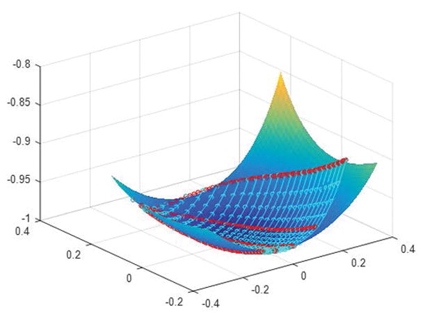
Visualization of the projected 3D randomized SVD space of the coarse MRF-FISP dictionary, fitted with a degree 5 polynomial. The 3 axes are the 3 singular vectors used for approximation. Each cyan curve represents a unique T₁ value and each red curve represents a unique T₂ value. The cyan and red circles represent the fitted values along different T₁ and T₂ curves, partitioning evenly each T₁, T₂ coarse level segment into 4 parts.

For a reconstructed voxel signal evolution x obtained from an MRF-FISP sequence scan, the signal evolution is first projected to the k-dimensional randomized SVD space by x̂ = U^*x. The projected signal evolution x̂ is then matched against all the T₁, T₂ fine grid points obtained above using maximal correlation to identify the largest two coarse values (corresponding to the coarse dictionary) for each tissue property parameter. Next, we examine the two fitted and refined adjacent T₁ curves between the two fitted adjacent T₂ curves and find on each T₁ curve the point with the largest correlation with x̂. Record the indices of these two points on the two T₁ curves as i and j with i,j = 1, …, p+1, where is the number of partitions on each curve. Then the T₂ value corresponding to x can be estimated as

$$\alpha T_{2,1}+(1-\alpha )T_{2,2},$$

with $\alpha =1-\frac{i+j-2}{2p}$, where T_2,1 and T_2,2 are the T₂ values corresponding to the two T₂ curves. The T₁ value corresponding to x can be estimated similarly.

Thanks to the random embedding of the randomized SVD, MRF dictionary fitting can approximate fine MRF parameter maps well enough as long as the original dictionary is not too coarse so as to avoid a wrong initial guess. It can also be easily generalized to the case where dictionaries consist of more tissue property parameters.

Methods

A. Compressed MRF with Randomized SVD

To demonstrate that our rSVD-MRF method works independently of the MRF sequence parameters and sampling pattern used, we use two types of MRF sequences, an MRF-FISP sequence with accelerated spiral readout and an MRF-bSSFP sequence with fully sampled multi-shot Cartesian readout, to evaluate the performance of the method. Specifically, we use these two MRF sequences to scan in vivo human-brain data and simulate MRF dictionaries. Note that these two MRF sequences have different parameters, which results in completely different behaviors in the spectrum of the MRF dictionaries.

The full MRF-FISP dictionary simulated contains 3,000 time frames and 5,970 different tissue property combinations with T₁ values ranging from 10ms to 2,950ms and T₂ values ranging from 2ms to 500ms with the constraint T₂ ≤ T₁ as shown in Table 1. A healthy volunteer was scanned on a Siemens Skyra 3T scanner (Siemens Healthcare, Erlangen, Germany) with a 20-channel head receiver coil array for 45 seconds using the MRF-FISP sequence and spiral sampling pattern with an acceleration factor of 48 (one out of 48 spiral interleaves per repetition MRF-FISP acquisition), a matrix size of 256 × 256, and a field of view (FOV) of 30 × 30cm². The collected spiral data for each coil were reconstructed using the non-uniform fast Fourier transform (NUFFT) (23) with an independently measured spiral trajectory to correct the gradient imperfection (24). Reconstructed images from all individual coils were then combined using the adaptive coil combination method (25), and scaled to the coil sensitivity map to compensate for the image intensity variation due to coil sensitivity (26). The T₁ and T₂ maps using rSVD-MRF can now be obtained following Figure 1, and the full T₁ and T₂ maps can be obtained through standard MRF pattern matching as the ground truth for comparison. We choose in this case the low rank index k = 30, and the power iteration index q = 0, since it has been shown in the literature that the singular values for MRF-FISP dictionaries decay rapidly (16).

Table 1.

Ranges and step sizes for T₁ and T₂ in the MRF-FISP dictionary. All values in milliseconds (ms).

FISP	Range	Step Size
T1	[10, 85]	5
	[90, 990]	10
	[1000, 1480]	20
	[1500, 2000]	50
	[2050, 2950]	100
T2	[2, 8]	2
	[10, 145]	5
	[150, 190]	10
	[200, 500]	50

The full MRF-bSSFP dictionary we use contains 500 time frames, 3,312 different tissue property combinations with T₁ values ranging from 20ms to 5,900ms, T₂ values ranging from 5ms to 2,900ms with the constraint T₂ ≤ T₁, as shown in Table 2, and off-resonance frequencies ranging from −300Hz to 300Hz with a step size of 4Hz. A healthy volunteer was scanned on a Siemens Espree 1.5T scanner (Siemens Healthcare, Erlangen, Germany) with a 4-channel head receiver coil array for 20 minutes using the MRF-bSSFP sequence with the conventional multi-shot Cartesian sampling pattern with no acceleration, a matrix size of 128 × 128 and a field-of-view of 25 × 25cm². The collected data for each coil were reconstructed using standard inverse fast Fourier transform (FFT). The reconstructed images from individual coils were then combined together and compensated for coil sensitivity. It has been shown in (16) that the singular values of MRF-bSSFP dictionaries stay relatively flat. Therefore, we choose the low rank index k = 100. In addition, we compare the performance of rSVD-MRF by varying the power iteration index q.

Table 2.

Ranges and step sizes for T₁ and T₂ for the MRF-bSSFP dictionary. All values in milliseconds (ms).

bSSFP	Range	Step Size
T1	[20, 1980]	20
	[2000, 5900]	300
T2	[5, 95]	5
	[100, 400]	50
	[500, 2900]	200

To demonstrate the efficiency of our randomized SVD approach, we further test its memory consumption for both MRF sequences and compare with the conventional MRF with the SVD approach (16) in MATLAB 2015b (The MathWorks, Natick, MA) with the assistance of the memory profiler function on a Windows 10 system with an Intel Xeon 2.6 GHz CPU (Intel Corporation, Santa Clara, CA) and 64 Gb of memory.

B. Dictionary Fitting

To evaluated the performance of our proposed low rank approximation approach using dictionary polynomial fitting combined with randomized SVD, we use the MRF-FISP sequence to simulate two MRF dictionaries, one coarse and one fine, and collect in vivo human-brain data from a healthy volunteer for comparison. We fit a polynomial to the coarse dictionary and compare the T₁, T₂ maps with the results obtained from the fine dictionary.

The coarse MRF-FISP dictionary is simulated according to the Bloch equations for 3,000 time frames with T₁ values varying from 20ms to 1,940ms with a step size of 80ms and T₂ values varying from 10ms to 170ms with a step size of 40ms with the restriction T₂ ≤ T₁, resulting in a dictionary of size 3,000 × 119. The fine MRF-FISP dictionary has the same number of time frames and the same T₁, T₂ ranges but with a 4 times finer step size. The step sizes for T₁ and T₂ values are 20ms and 10ms respectively, resulting in a dictionary of size 3,000 × 1,585. The in vivo brain scan of a healthy volunteer was obtained on a Siemens Skyra 3T scanner (Siemens Healthcare, Erlangen, Germany) with a 20-channel head receiver coil array using the MRF-FISP sequence and spiral sampling pattern with an acceleration factor of 48 (one out of 48 spiral interleaves per repetition MRF-FISP acquisition), a matrix size of 256 × 256, and a FOV of 30 × 30cm². The collected spiral data for each coil were reconstructed using the NUFFT with an independently measured spiral trajectory for gradient imperfection correction. Reconstructed images from all individual coils were then combined and compensated for coil sensitivity variation. In addition, to apply polynomial fitting with randomized SVD, we set the rank of approximation for the randomized SVD to k = 3, the power iteration index to q = 0, the degree of the fitting polynomial to d = 5, and the fineness index to t = 4. Note that rank k and degree of polynomial d can be varied, as long as they satisfy the condition $\left(\begin{array}{c}k+d\\ d\end{array}\right)\le n$ from the Theory section. Moreover, we set t = 4 since the benchmark fine dictionary is 4 times finer than the coarse dictionary. The T₁ and T₂ maps can then be calculated following the procedure described in the Theory section above and compared against the rSVD-MRF results using both the coarse dictionary and the fine dictionary.

Note that informed consent was obtained before each scan and all experiments were approved by our institutional review board (IRB).

Results

Figure 3 shows the results of applying the rSVD-MRF with power iteration index q = 0 to a scanned healthy volunteer brain dataset with an MRF-FISP dictionary with full resolution. Specifically, the reconstructed T₁, T₂ parameter maps and the difference maps using the direct MRF method and the rSVD-MRF method with rank k = 10 and k = 30 using the MRF-FISP sequence are displayed. The range of the T₁ values displayed is 10ms to 2,500ms (anything beyond 2,500ms is displayed as 2,500ms), while the range of the T₂ value displayed is 2ms to 250ms for a better visualization (anything beyond 250ms is displayed as 250ms). In addition, the difference maps for both T₁ and T₂ values are scaled up 10 times. The difference maps clearly demonstrate that the T₁ and T₂ maps from rSVD-MRF are in good agreement with the ground truth MRF maps, even though we have only used 1% (30 out of 3,000) of the principal components. Explicitly, the relative error (the ratio between the Frobenius norm of the difference map and that of the ground truth map) between the T₁ maps from rSVD-MRF and the ground truth is only 0.58%; while the relative error between the T₂ maps is 1.09%. On the other hand, the performance of rSVD-MRF starts to break down if one pushes too much. For instance, when we choose rank k = 10, the relative error increases to 5% for T₁ maps, and to 11.66% for T₂ maps.

Figure 3.

Performance of rSVD-MRF on MRF-FISP sequence. Top: T₁ maps. Bottom: T₂ maps. Column (a): MRF maps without compression. Column (b): MRF maps using rSVD-MRF with k = 10. Column (c): MRF maps using rSVD-MRF with k = 30. Column (d): difference maps between columns (a) and (b). Column (e): difference maps between columns (a) and (c). Column (f): Reconstruction fidelity comparison between SVD and rSVD, both against MRF maps without compression.

We further show in Figure 3(f) the comparison of the reconstruction fidelity of T₁ and T₂ maps using rSVD and the conventional SVD method. Both methods are compared with the ground truth MRF maps without compression with rank k varying from 5 to 50. The results from the rSVD method is averaged over 100 runs with standard deviation plotted. One can see from the plots that the relative error curves for both T₁ and T₂ maps using rSVD agree with the relative error curves using SVD when rank k is not chosen too small.

The results of applying the rSVD-MRF method with no power iteration (q = 0) to the in vivo brain data of a healthy volunteer and the MRF dictionary using the MRF-bSSFP sequence are shown in Figure 4. Here we show the T1, T2, and off-resonance maps computed using both conventional MRF and the rSVD-MRF method with no power iteration. The left column of images corresponds to the T₁, T₂ and off-resonance maps using the conventional MRF. The middle column of images contains the T₁, T₂ and off-resonance maps using the rSVD-MRF method with no power iteration. The last column of images are the difference maps between the two approaches. For better visualization, the T1 values between 20ms and 5,000ms are displayed and the T1 difference map is scaled up 10 times; the T2 values between 5ms and 250ms are displayed and the T2 difference map is scaled up 2.5 times; the off-resonance values between −100Hz and 100Hz are displayed. Although we have taken 20% of the principal components (100 out of 500), the difference maps exhibit a larger residual as compared to the FISP results due to the slower decay of the singular values in the bSSFP dictionary.

Figure 4.

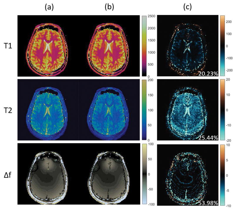
Performance of randomized SVD on MRF-bSSFP sequence with rank k = 100 and power iteration index q = 0. Top to bottom: T₁ maps, T₂ maps, and off-resonance maps. Column (a): MRF maps without compression. Column (b): MRF maps with randomized SVD with k = 100 and q = 0. Column (c): difference maps between the two cases.

To remediate this problem, we set the power iteration index q = 2. We notice that using q = 2 provides a better approximation performance compared to the case q = 0, without introducing too much computational overhead. The T₁ and T₂ maps can now be obtained following Figure 1 and compared against the results obtained from the standard MRF approach, as shown in Figure 5. Again, the maps for the standard MRF are shown in the first column, the maps for the rSVD-MRF are shown in the second column, and the difference maps are shown in the last column. By comparing the difference maps, the residuals are much smaller than that of the case when there is no power iteration involved. This demonstrates that the approximation error can be diminished significantly by incorporating a nonzero power iteration index when the singular value decay is not fast enough. Typically, setting the power iteration index q = 2 is enough, as we have seen no significant improvement in in vivo experiments when setting q = 3 and higher.

Figure 5.

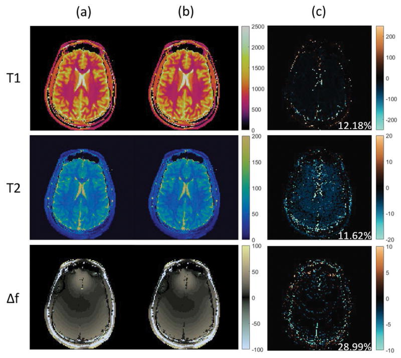
Performance of randomized SVD on MRF-bSSFP sequence with rank k = 100 and power iteration index q = 2. Top to bottom: T₁ maps, T₂ maps, and off-resonance maps. Column (a): MRF maps without compression. Column (b): MRF maps with randomized SVD with k = 100 and q = 2. Column (c): difference maps between the two cases.

To demonstrate the advantage of the rSVD-MRF method, the memory consumption details calculated from the memory profiler of MATLAB are shown in Table 3. The memory savings for calculating the SVD approximation to the MRF-FISP dictionary is almost 1,000 times using our rSVD-MRF method against the standard MRF with SVD approach. For the MRF-bSSFP calculation using rSVD-MRF, we still get decent memory savings around 15 times compared to the MRF using SVD with or without power iteration, although not as significant as the MRF-FISP case.

Table 3.

Memory consumption for calculating dictionaries with randomized SVD and direct SVD approach.

	Direct Calculation	rSVD-MRF (q=0)	rSVD-MRF (q=2)
MRF-FISP	1,028.8Mb	1.6Mb	N/A
MRF-bSSFP	11,571Mb	764Mb	769.5Mb

We next demonstrate the possibility of constructing accurate tissue property maps from coarse MRF dictionaries combining rSVD-MRF with polynomial fitting. Figure 2 shows a 3D visualization of the projected randomized SVD space of the coarse MRF-FISP dictionary with rank k = 3, fitted with a degree d = 5 polynomial, and fineness index t = 4. The cyan and red curves represent different T₁ and T₂ values respectively, and the circles represent fitted values along each curve, partitioning each T₁, T₂ coarse grid into 4 segments. The figure shows that the polynomial surface fits the projected coarse dictionary perfectly with fitting statistics R² = 1 and adjusted R²=0.99.

The MRF results with different dictionaries are shown in Figure 6 and Figure 7. In Figure 6, the T₁ and T₂ maps of the scanned human brain are obtained via the projected fine dictionary, the projected coarse dictionary, the projected coarse dictionary interpolated with piecewise linear functions, and the projected coarse dictionary fitted with a degree 5 polynomial respectively. We see a clear quality degradation when the dictionary is coarse. In particular, note that the T₂ map obtained from the coarse dictionary shows significant loss of detail and exhibits a flat image appearance. This, however, is remediated by fitting a polynomial to the coarse dictionary lattice. The results are more clearly displayed in the difference maps in Figure 7, where the T₁, T₂ difference maps between the coarse and fine dictionaries approaches, the piecewise linear interpolated and the fine dictionary approaches, and the fitted and fine dictionary approaches are shown in the left, middle, and right columns respectively. The T₁, T₂ map differences between the coarse dictionary and the 4 times finer dictionary are significantly diminished by polynomial fitting in the rank 3 randomized SVD space. Specially, the relative error decreases from 3.68% to 2.06% for the T₁ map, and from 14.37% to 7.40% for the T₂ map. One may also notice that the piecewise linear interpolation method also beats the coarse dictionary approach. Its performance, however, is not as good as that of the polynomial fitting approach. In particular, the T₂ map obtained from piecewise linear interpolation still exhibits certain degree of flat pattern in the white matter region.

Figure 6.

T₁, T₂ maps of a brain data against different MRF-FISP dictionaries. First row: T₁ maps. Second row: T₂ maps. Column (a): MRF with compressed fine dictionary. Column (b): MRF with compressed coarse dictionary. Column (c): MRF with piecewise linear interpolated compressed coarse dictionary. Column (d): MRF with polynomial fitted compressed coarse dictionary.

Figure 7.

T₁, T₂ difference maps of a brain data between different MRF-FISP dictionaries. First row: T₁ map differences. Second row: T₂ map differences. Column (a): difference maps between the coarse dictionary and the fine dictionary. Column (b): difference maps between the piecewise linear interpolated coarse dictionary and the fine dictionary. Column (c): difference maps between the polynomial fitted coarse dictionary and the fine dictionary. Note the scaling factor changes in both T₁ and T₂ cases.

Discussion and Conclusions

This work studies new low rank approximation approaches, namely, compressed MRF with randomized SVD (rSVD-MRF) and dictionary fitting with polynomials in the MRF framework. It provides useful tools for large sized MRF problems when fine MRF dictionaries are needed or multi-component such as chemical exchange effects are considered, where calculating the dictionaries or applying conventional compression methods such as the SVD is infeasible. Specifically, instead of calculating and compressing the whole MRF dictionary, and then throw away most of the components that are not important to obtain a low rank approximation, rSVD-MRF calculates only one tissue property signal evolution at a time to update the low rank approximant to the MRF dictionary, and discards it afterwards. This results in up to 1,000 times memory savings for calculating MRF dictionaries, which makes it possible to handle large sized MRF problems that had been previously prohibitive.

Furthermore, when combined with polynomial fitting in the low rank randomized SVD space, it enables us to fit the low rank approximation of a coarse MRF dictionary to certain degree polynomials and generate arbitrary fine resolution MRF maps close to the maps from a fine MRF dictionary. This in return can further reduce the memory requirement for generating high resolution MRF maps, as well as speed up the whole process. Moreover, it is possible to provide more accurate maps than the given fine dictionary because of the smoothness of polynomial fitting and the arbitrary number of partitions one can make within each coarse grid. This idea could essentially remove dictionary resolution as a limitation in MRF. Note that although we have only demonstrated the two-component case for T₁ and T₂ values, it can be easily extended to problems with more components. Therefore, we see great potential in this approach being applied to multi-parameter large scale MRF problems, such as MRF-X (13) for multi-component chemical exchange effects.

References

- 1.Ma D, Fulani V, Seiberlich N, Liu K, Sunshine JL, Duerk JL, Griswold MA. Magnetic resonance fingerprinting. Nature. 2013;495:187–192. doi: 10.1038/nature11971. [DOI] [PMC free article] [PubMed] [Google Scholar]
- 2.Cloos MA, Zhao T, Knoll F, Alon L, Lattanzi R, Sodickson DK. Magnetic Resonance Fingerprint Compression. Proc Intl Soc Mag Reson Med. 2015;23 Abstract 0330. [Google Scholar]
- 3.Gómez PA, Buonincontri G, Molina-Romero M, Ulas C, Sperl JI, Menzel MI, Menze BH. 3D magnetic resonance fingerprinting with a clustered spatiotemporal dictionary. Proc Intl Soc Mag Reson Med. 2016;24 Abstract 0251. [Google Scholar]
- 4.Chen Y, Pahwa S, Hamilton JI, Dastmalchian S, Plecha D, Seiberlich N, Griswold MA, Fulani V. 3D Magnetic Resonance Fingerprinting for Quantitative Breast Imaging. Proc Intl Soc Mag Reson Med. 2016;24 Abstract 0399. [Google Scholar]
- 5.Cohen O, Sarracanie M, Rosen MS, Ackerman JL. In Vivo Optimized Fast MR Fingerprinting in the Human Brain. Proc Intl Soc Mag Reson Med. 2016;24 Abstract 0430. [Google Scholar]
- 6.Doneva M, Amthor T, Koken P, Sommer K, Börnert P. Low Rank Matrix Completion-based Reconstruction for Undersampled Magnetic Resonance Fingerprinting Data. Proc Intl Soc Mag Reson Med. 2016;24 doi: 10.1016/j.mri.2017.02.007. Abstract 0432. [DOI] [PubMed] [Google Scholar]
- 7.Cline CC, Chen X, Mailhe B, Wang Q, Nadar M. AIR-MRF: Accelerated iterative reconstruction for magnetic resonance fingerprinting. Proc Intl Soc Mag Reson Med. 2016;24 doi: 10.1016/j.mri.2017.07.007. Abstract 0434. [DOI] [PubMed] [Google Scholar]
- 8.Zhang X, Li R, Hu X. MR Fingerprinting Reconstruction with Kalman Filter. Proc Intl Soc Mag Reson Med. 2016;24 doi: 10.1016/j.mri.2017.04.004. Abstract 0436. [DOI] [PubMed] [Google Scholar]
- 9.Chen Y, Mehta B, Hamilton JI, Ma D, Seiberlich N, Griswold MA, Fulani V. Free-Breathing 3D Abdominal Magnetic Resonance Fingerprinting Using Navigators. Proc Intl Soc Mag Reson Med. 2016;24 Abstract 0716. [Google Scholar]
- 10.Zhao B, Setsompop K, Gagoski B, Ye H, Adalsteinsson E, Grant PE, Wald LL. A Model-Based Approach to Accelerated Magnetic Resonance Fingerprinting Time Series Reconstruction. Proc Intl Soc Mag Reson Med. 2016;24 Abstract 0871. [Google Scholar]
- 11.Pahwa S, Lu Z, Dastmalchian S, Jiang Y, Patel M, Meropol N, Griswold MA, Fulani V. Application of Magnetic Resonance Fingerprinting (MRF) for Assessment of Rectal Cancer: A Feasibility Study. Proc Intl Soc Mag Reson Med. 2016;24 Abstract 2966. [Google Scholar]
- 12.Zhao B, Haldar JP, Setsompop K, Wald LL. Optimal experiment design for magnetic resonance fingerprinting. 2016 38th Annual International Conference of the IEEE Engineering in Medicine and Biology Society (EMBC); Orlando, FL. 2016. pp. 453–456. [DOI] [PMC free article] [PubMed] [Google Scholar]
- 13.Hamilton JI, Deshmane A, Griswold MA, Seiberlich N. MR Fingerprinting with Chemical Exchange (MRF-X) for In Vivo Multi-Compartment Relaxation and Exchange Rate Mapping. Proc Intl Soc Mag Reson Med. 2016;24 Abstract 0431. [Google Scholar]
- 14.Buonincontri G, Sawiak SJ. MR fingerprinting with simultaneous B1 estimation. Magn Reson Med. 2016;76:1127–1135. doi: 10.1002/mrm.26009. [DOI] [PMC free article] [PubMed] [Google Scholar]
- 15.Cloos MA, Knoll F, Zhao T, Block KT, Bruno M, Wiggins GC, Sodickson DK. Multiparametric imaging with heterogeneous radiofrequency fields. Nature Communications. 2016;7:12445. doi: 10.1038/ncomms12445. [DOI] [PMC free article] [PubMed] [Google Scholar]
- 16.McGivney DF, Pierre E, Ma D, Jiang Y, Saybasili H, Fulani V, Griswold MA. SVD compression for magnetic resonance fingerprinting in the time domain. IEEE Transactions on Medical Imaging. 2014 Dec;33(12):2311–2322. doi: 10.1109/TMI.2014.2337321. [DOI] [PMC free article] [PubMed] [Google Scholar]
- 17.Jiang Y, Ma D, Seiberlich N, Fulani V, Griswold MA. MR fingerprinting using fast imaging with steady state precession (FISP) with spiral readout. Magnetic Resonance in Medicine. 2015;74(6):1621–1631. doi: 10.1002/mrm.25559. [DOI] [PMC free article] [PubMed] [Google Scholar]
- 18.Schmitt P, Griswold MA, Fulani V, Haase A, Flentje M, Jakob PM. A simple geometrical description of the TrueFISP ideal transient and steady-state signal. Magn Reson Med. 2006;55:177–186. doi: 10.1002/mrm.20738. [DOI] [PubMed] [Google Scholar]
- 19.Trefethen LN, Bau D., III . Numerical linear algebra. Philadelphia: Society for Industrial and Applied Mathematics; 1997. [Google Scholar]
- 20.Cauley SF, Setsompop K, Ma D, Jiang Y, Ye H, Adalsteinsson E, Griswold MA, Wald LL. Fast Group Matching for MR Fingerprinting Reconstruction. Magn Reson Med. 2015;74:523–528. doi: 10.1002/mrm.25439. [DOI] [PMC free article] [PubMed] [Google Scholar]
- 21.Halko N, Martinsson PG, Tropp JA. Finding structure with randomness: Probabilistic algorithms for constructing approximate matrix decompositions. SIAM Review. 2011;53(2):217–288. [Google Scholar]
- 22.Johnson WB, Lindenstrauss J. Extensions of Lipschitz mappings into a Hilbert space. Contemporary Mathematics. 1984;26:189–206. [Google Scholar]
- 23.Fessler JA, Sutton BP. Nonuniform fast fourier transforms using min-max interpolation. IEEE Trans Signal Process. 2003;51:560–574. [Google Scholar]
- 24.Duyn JH, Yang Y, Frank JA, van der Veen JW. Simple correction method for k-space trajectory deviations in MRI. J Magn Reson. 1998;132:150–3. doi: 10.1006/jmre.1998.1396. [DOI] [PubMed] [Google Scholar]
- 25.Walsh DO, Gmitro AF, Marcellin MW. Adaptive reconstruction of phased array MR imagery. Magn Reson Med. 2000;43:682–90. doi: 10.1002/(sici)1522-2594(200005)43:5<682::aid-mrm10>3.0.co;2-g. [DOI] [PubMed] [Google Scholar]
- 26.Griswold MA, Walsh D, Heidemann RM, Haase A, Jakob P. The Use of an Adaptive Reconstruction for Array Coil Sensitivity Mapping and Intensity Normalization. Proc Tenth Sci Meet Int Soc Magn Reson Med. 2002:2410. [Google Scholar]