Feature-coding transitions to conjunction-coding with progression through human visual cortex

We use a novel analysis of neuroimaging data to assess representations throughout visual cortex, revealing a transition from feature-coding to conjunction-coding along both ventral and dorsal pathways. Occipital cortex contains more information about spatial frequency and contour than about conjunctions of those features, whereas inferotemporal and parietal cortices contain conjunction coding sites in which there is more information about the whole stimulus than its component parts.

Abstract

Identifying an object and distinguishing it from similar items depends upon the ability to perceive its component parts as conjoined into a cohesive whole, but the brain mechanisms underlying this ability remain elusive. The ventral visual processing pathway in primates is organized hierarchically: Neuronal responses in early stages are sensitive to the manipulation of simple visual features, whereas neuronal responses in subsequent stages are tuned to increasingly complex stimulus attributes. It is widely assumed that feature-coding dominates in early visual cortex whereas later visual regions employ conjunction-coding in which object representations are different from the sum of their simple feature parts. However, no study in humans has demonstrated that putative object-level codes in higher visual cortex cannot be accounted for by feature-coding and that putative feature codes in regions prior to ventral temporal cortex are not equally well characterized as object-level codes. Thus the existence of a transition from feature- to conjunction-coding in human visual cortex remains unconfirmed, and if a transition does occur its location remains unknown. By employing multivariate analysis of functional imaging data, we measure both feature-coding and conjunction-coding directly, using the same set of visual stimuli, and pit them against each other to reveal the relative dominance of one vs. the other throughout cortex. Our results reveal a transition from feature-coding in early visual cortex to conjunction-coding in both inferior temporal and posterior parietal cortices. This novel method enables the use of experimentally controlled stimulus features to investigate population-level feature and conjunction codes throughout human cortex.

NEW & NOTEWORTHY We use a novel analysis of neuroimaging data to assess representations throughout visual cortex, revealing a transition from feature-coding to conjunction-coding along both ventral and dorsal pathways. Occipital cortex contains more information about spatial frequency and contour than about conjunctions of those features, whereas inferotemporal and parietal cortices contain conjunction coding sites in which there is more information about the whole stimulus than its component parts.

object perception is underpinned by a hierarchical series of processing stages in the ventral visual pathway (Felleman and Van Essen 1991; Hubel and Wiesel 1965; Kobatake and Tanaka 1994). At each successive stage from primary visual cortex (V1) to anterior inferotemporal (aIT) cortex, the complexity of the optimal stimuli increases: neurons in V1 are tuned to simple stimulus attributes such as orientation (Hubel and Wiesel 1965; Mazer et al. 2002); neurons in V4 and posterior inferotemporal cortex (pIT) are selective for moderately complex features (Brincat and Connor 2004; Kobatake and Tanaka 1994; Pasupathy and Connor 1999; Rust and DiCarlo 2010); and neurons in aIT prefer partial or complete views of complex objects (Desimone et al. 1984; Kobatake and Tanaka 1994; Tanaka 1996). Data from functional magnetic resonance imaging (fMRI) in humans corroborate these findings: the blood oxygenation level-dependent (BOLD) signal exhibits selectivity for orientation, spatial frequency, and color in early visual regions (Brouwer and Heeger 2009; Henriksson et al. 2008; Kamitani and Tong 2005; Serences et al. 2009) but is sensitive to object-level properties such as global contour or object category in higher visual regions (Drucker and Aguirre 2009; Kanwisher et al. Chun 1997; Kriegeskorte et al. 2008; Malach et al. 1995; Ostwald et al. 2008). It is widely assumed that downstream, object-specific representations are constructed through combination of the simple feature representations upstream, but the manner in which this combination occurs remains unknown.

There are at least three possible combination schemes. The first assumes that downstream object-level representations perform “and-like” operations on upstream feature representations (Rust and DiCarlo 2012), transforming the feature code into conjunction-sensitive representations in inferotemporal (IT) cortex. This feature-to-conjunction transition scheme is assumed by many models of object processing (Bussey and Saksida 2002; Cowell et al. 2010; Fukushima 1980; Perrett and Oram 1993; Riesenhuber and Poggio 1999; Serre et al. 2007; Wallis and Rolls 1997) and accords with electrophysiological findings of IT neurons selective for complex objects (Desimone et al. 1984; Fujita et al. Cheng 1992; Kobatake and Tanaka 1994). However, when tested with large stimulus sets many IT neurons show broad tuning, responding to multiple complex objects (Desimone et al. 1984; Kreiman et al. 2006; Zoccolan et al. 2007). Therefore, apparent object-level selectivity in an IT neuron tested with a small stimulus set might instead reflect selectivity for a low-level feature possessed by only a few objects in the set. Thus the data do not rule out a second scheme: a global feature-coding hypothesis, in which simple features are coded separately in visual cortex and are bound by the synchronization of neural activity rather than by convergence onto a cortically localized representation of the conjunction (Eckhorn 1999a, 1999b; Singer and Gray 1995). Finally, a third possible coding scheme is a global conjunction-coding hypothesis, in which all stations in the hierarchy bind simple features together nonlinearly to produce conjunctions (Shigihara and Zeki 2013, 2014). Under this scheme, the apparent feature selectivity of early visual cortex belies a neural code that is optimized for discriminating complex objects that contain those features. Supporting this account, several studies have reported coding of simple conjunctions of features such as color, form, motion, and orientation in early visual regions (Anzai et al. 2007; Engel 2005; Gegenfurtner et al. 1997; Johnson et al. 2008; Seymour et al. 2009, 2010) and coding of complex conjunctions in both early and higher-level visual regions (Erez et al. 2016).

To differentiate between the three alternative schemes, we must measure not just the presence of feature-coding and conjunction-coding throughout visual cortex but the relative contribution of each. Using fMRI in humans, we devised a novel stimulus set and multivariate pattern analysis (MVPA) technique to pit feature-coding against conjunction-coding. We created stimuli by building conjunctions from binary features, thereby allowing each cortical region to be probed for information at two levels: features or conjunctions. Feature information and conjunction information were assessed with the same neuroimaging data set and placed in a ratio, allowing direct comparison of the two coding schemes throughout cortex.

MATERIALS AND METHODS

Methods Overview

Participants in the scanner viewed visual stimuli constructed hierarchically from four binary features to give 16 unique, conjunctive objects. We verified by means of a one-back repetition detection task that participants were attending to the stimuli sufficiently well to discriminate between distinct objects, i.e., between different unique conjunctions of features (Table 1). We used a support vector machine (SVM) to classify patterns of BOLD responses evoked by the stimuli. For each session in each subject, we constructed four 2-way feature-level SVM classifiers (1 classifier for each binary feature) and one 16-way object-level SVM classifier (Fig. 1). This yielded both feature- and object-level classification accuracy for a given region of interest (ROI) (Tables 2 and 3). We next constructed a feature conjunction index (FCI) for each ROI by comparing the output of the feature- and object-level classifiers (Fig. 1; Table 4). A positive FCI indicates that the ROI contains more information about individual objects than is predicted from the information it contains about the separate object features, suggesting that its activation pattern is modulated by the presence or absence of specific objects rather than by individual features. A negative FCI indicates that the ROI contains more information about individual features than about whole objects, suggesting that voxel activations are primarily modulated by individual feature dimensions rather than by whole object identity. These interpretations of FCI were confirmed via analyses of synthetic data.

Table 1.

Behavioral performance in the scanner

	Scan Session 1	Scan Session 2
Mean proportion correct	0.903 (±0.0185)	0.947 (±0.00894)
Mean arcsine(proportion correct)	1.27 (±0.0350)	1.35 (±0.0214)

Values are mean (±SE) accuracy on the 1-back repetition-detection task performed in the scanner across subjects. A t-test comparing the arcsine-transformed proportion correct scores indicated that performance was reliably better in scan session 2 (P = 0.0138).

Fig. 1.

Stimulus construction, task protocol, and multivariate pattern classifiers. A: stimulus construction. The 4 binary features from which the 16 object-level stimuli are composed (full stimulus set shown in D). Each feature has 2 possible values, A and B. B: task protocol. In each scan session, participants completed 10 experimental runs, each lasting 264 s (44 trials of 6-s duration). A run contained 34–36 stimulus trials (2 presentations each of the 16 stimuli in the set, ordered pseudorandomly, in addition to 2–4 stimuli chosen pseudorandomly from the set and inserted to create immediate repeats) and 8–10 null trials. On stimulus presentation trials, the fixation point was red, stimulus duration was 3 s, and the interstimulus interval varied between 2.5 and 3.5 s; participants performed a 1-back repetition-detection task. On null trials, the fixation point changed to green; participants indicated by button press when they detected a slight dimming of the fixation point, which occurred once or twice per null trial. Participants also completed several sessions of visual search training between the 2 scans, but we detected no effect of training on our measure of feature- and conjunction-coding (feature conjunction index, FCI) in cortex. C: feature classification. Four separate feature classifiers were trained, 1 for each binary feature defined in the stimulus set. The 4 feature classification problems are shown in the 4 panels (Right Spatial Frequency, Right Outline, Left Spatial Frequency, Left Outline) in which the designation of stimuli to feature categories is indicated with red and green boxes. Classifiers used a support vector machine trained with hold-one-out cross-validation. D: object classification. A single object-level classifier was trained to classify the stimuli into 16 categories, each corresponding to a unique stimulus. E: calculation of the FCI. The product of the 4 feature-level accuracies was used to predict—independently for each trial—the accuracy of a hypothetical object-level classifier whose performance depends only on feature-level information. On each trial, the 4 feature-classifier responses (defined as 0 or 1 for incorrect or correct) were multiplied to produce a value of 0 or 1 (incorrect or correct) for the hypothetical object-level classifier. Next, the empirically observed object-level classifier accuracy (derived from the 16-way conjunction classifier) and the hypothetical object-level accuracy (predicted from the 4 feature classifiers) were averaged over trials and placed in a log ratio (Eq. 1). When the empirically observed object classifier accuracy exceeds the hypothetical object accuracy predicted from feature classifier accuracies, FCI is positive; when the feature classifier accuracies predict better object-level knowledge accuracy than is obtained by the object classifier, FCI is negative (see Fig. 2).

Table 2.

Feature-level classifier accuracy for each feature type and mean across all feature types

	Ventral Stream				Dorsal Stream
	V1	V2v	V3v	LOC	V2d	V3d
Feat 1 (SF1)	0.791 (±0.0261)	0.722 (±0.0254)	0.686 (±0.0178)	0.516 (± 0.0051)	0.689 (±0.0237)	0.652 (±0.0195)
Feat 2 (Outline1)	0.864 (±0.0163)	0.675 (±0.0188)	0.609 (±0.0186)	0.550 (±0.0101)	0.777 (±0.0239)	0.618 (±0.0203)
Feat 3 (SF2)	0.773 (±0.0235)	0.679 (±0.0204)	0.658 (±0.0178)	0.526 (±0.0092)	0.685 (±0.0211)	0.653 (±0.0206)
Feat 4 (Outline2)	0.853 (±0.0160)	0.678 (±0.0223)	0.657 (±0.0176)	0.557 (±0.0062)	0.736 (±0.0240)	0.692 (±0.0280)
Overall mean acc.	0.820 (±0.0186)	0.688 (±0.0186)	0.653 (± 0.0121)	0.537 (±0.00266)	0.722 (±0.02)	0.653 (±0.0146)
95% CI around overall mean	[0.815, 0.825]	[0.682, 0.695]	[0.646, 0.659]	[0.530, 0.544]	[0.716, 0.728]	[0.647, 0.66]

In both ventral and dorsal streams, 1st 4 rows show mean (±SE) across subjects of the feature-level classifier accuracy for each feature type across subjects. Chance = 0.5. SF,  spatial frequency. Fifth row shows overall mean ± SE accuracy across all 4 feature-level classifiers  across subjects. Sixth row shows 95% CIs around the overall mean accuracy determined by within-subject bootstrap resampling with replacement over 10,000 iterations. All data were averaged over 2 sessions for each subject. Overall mean accuracy scores for each session in each subject were transformed into a log-likelihood ratio (log odds; chance = 0) and submitted to a 2-way repeated-measures ANOVA, with factors Scan Session (1, 2) and ROI (V1, V2v, V3v, V2d, V3d, LOC), revealing a main effect of ROI [F(5,35) = 83.14, P < 0.001, η² = 0.922], no significant effect of Scan Session [F(1,7) = 0.860, P = 0.39, η² = 0.109], and a nonsignificant interaction [F(5,35) = 2.367, P = 0.06, η² = 0.253]. Accuracy was lowest in region LOC, but a 1-sample t-test revealed that the log odds of LOC accuracy (collapsed over sessions) exceeded chance performance (mean = 0.1486, SD = 0.0303, t[7] = 13.89, P < 0.001).

Table 3.

Object-level classifier accuracy

	Ventral Stream				Dorsal Stream
	V1	V2v	V3v	LOC	V2d	V3d
Mean accuracy	0.292 (±0.0272)	0.200 (±0.0163)	0.154 (±0.0101)	0.0926 (±0.00701)	0.204 (±0.0208)	0.155 (±0.0131)
95% CI	[0.280, 0.304]	[0.189, 0.210]	[0.144, 0.164]	[0.0848, 0.101]	[0.193, 0.215]	[0.145, 0.164]

Values are mean (±SE) accuracy of object-level classifier by ROI (average over 2 sessions for each subject) across subjects and 95% confidence intervals (CIs) around the mean, determined by within-subject bootstrap resampling with replacement over 10,000 iterations. Chance = 0.0625. Accuracy scores for each session in each subject were transformed into a log-likelihood ratio (log odds; chance = −2.71) and submitted to a 2-way repeated-measures ANOVA, with factors Scan Session (1, 2) and ROI (V1, V2v, V3v, V2d, V3d, LOC), revealing a main effect of ROI [F(5,35) = 61.96, P < 0.001, η² = 0.90], no significant effect of Scan Session [F(1,7) = 0.312, P = 0.59, η² = 0.043], and no significant interaction [F(5,35) = 1.61, P = 0.183, η² = 0.187]. Accuracy was lowest in region LOC, but a 1-sample t-test revealed that the log odds of LOC accuracy (collapsed over sessions) exceeded chance performance (mean = −2.30, SD = 0.2321, t[7] = 4.95, P < 0.001).

Table 4.

Feature-conjunction index in visual cortical ROIs

	Ventral Stream				Dorsal Stream
	V1	V2v	V3v	LOC	V2d	V3d
Subject 1	−0.564	−0.081	−0.308	0.080	−0.207	−0.088
Subject 2	−0.467	−0.271	−0.137	0.188	−0.207	−0.085
Subject 3	−0.425	−0.251	−0.110	0.366	−0.298	−0.284
Subject 4	−0.476	−0.161	−0.284	0.391	−0.440	−0.313
Subject 5	−0.453	−0.301	−0.319	0.102	−0.497	−0.222
Subject 6	−0.464	−0.151	−0.148	−0.145	−0.396	−0.276
Subject 7	−0.584	−0.304	−0.209	−0.091	−0.345	0.055
Subject 8	−0.494	0.089	−0.133	−0.181	−0.418	−0.431
Mean FCI	−0.491	−0.179	−0.206	0.089	−0.351	−0.206
SE	0.020	0.048	0.030	0.078	0.038	0.055
95% CI	[−0.545, −0.442]	[−0.252, −0.110]	[−0.292, −0.125]	[−0.0558, 0.192]	[−0.422, −0.284]	[−0.293, −0.122]

Values are individual subjects’ FCI by ROI (average over 2 sessions for each subject), with mean and SE across subjects and 95% CIs determined by within-subject bootstrap sampling with replacement over 10,000 iterations (see materials and methods). Mean values are also shown graphically in Fig. 3.

Participants, Stimuli, Task, and Data Acquisition

Participants.

Eight healthy participants (4 women, 4 men) with normal or corrected-to-normal vision completed two scan sessions. All participants provided written informed consent to participate in protocols reviewed and approved by the Institutional Review Board at University of California, San Diego and were compensated at $20/h for fMRI scan sessions and $10/h for behavioral test sessions.

Stimulus and task parameters.

Motivated by evidence that the integration of contour elements into global shape (Brincat and Connor 2004) and local image features into global texture (Goda et al. 2014; Hiramatsu et al. 2011) are key mechanisms by which the ventral pathway constructs complex object representations, we created novel object stimuli by building conjunctions from binary features defined by contour and spatial frequency (Fig. 1). To examine whether conjunction-coding emerged from an upstream feature code, it was important to choose stimulus features that are encoded by early visual regions. Although shape contour is often considered a relatively high-level property of a visual stimulus and is known to be represented in areas like lateral occipital cortex (LOC), the binary contour features we used must be encoded as a collection of simple, oriented line segments in early visual regions such as V1 and V2, because of small receptive field (RF) size (see also Brincat and Connor 2006; Yau et al. 2013). The sensitivity of neurons in early visual cortex to spatial frequency is well documented (e.g., Foster et al. 1985; von der Heydt et al. 1992). Stimuli subtended ~7–10° of visual angle, except in one session in one participant (subject AF) in which they subtended ~5–7° (visual inspection of MVPA results did not give any indication of greater between-session differences in any of the MVPA measures for subject AF than for other subjects). Visual displays were presented to participants via back-projection onto a screen at the foot of the scanner bore, which was viewed in a mirror fixed to the head coil, over a distance of ~380 cm. To ensure that all pixel locations emitted the same average luminance over the course of a trial (and therefore that all stimuli possessed the same average luminance), visual stimuli cycled continuously from a positive to a negative image, with every pixel oscillating from minimum to maximum luminance according to a temporal sine wave with frequency of 2 Hz.

Each scan session contained 10 experimental task runs. Each task run lasted 274 s (44 trials lasting 6 s each, in addition to a 10-s posttask scanning window). Participants were instructed to fixate a circular colored fixation point that appeared at the center of the screen throughout all trials. Each run comprised 32 “stimulus” trials, 2–4 “immediate-repeat” trials, and 8–10 “null” trials. On stimulus and immediate-repeat trials, the fixation point was red and stimulus onset began 0.2–0.7 s after the start of the trial (with exact onset randomly jittered within that window); stimulus presentation lasted 3 s and was followed by a 2.3- to 2.8-s response window in which only the fixation point appeared, to give a total trial duration of 6 s. The variable cue onset time produced an interstimulus interval that varied between 2.5 and 3.5 s. The 32 stimulus trials comprised two pseudorandomly ordered presentations of each of the 16 unique stimuli. To generate immediate-repeat trials, a pseudorandomly chosen stimulus was inserted into the sequence such that it created a repeat of the stimulus in the immediately preceding trial; functional data from these trials were removed from multivariate analyses. On null trials, the fixation point changed from red to green and participants were required to press any button whenever they detected a slight dimming of the green fixation point, which could occur once or twice per null trial; a response was required within 1 s of each dimming event for a trial to be scored as correct. This task was designed to reduce the tendency for mind-wandering, known to affect baseline measures of BOLD (Stark and Squire 2001). Accuracy on null trials was monitored to ensure participant wakefulness, and the degree of fixation point dimming was adjusted between runs to produce below-ceiling performance such that attention was maintained. Participants performed a one-back repetition detection task, indicating by button press whether the stimulus was the same as (button 2) or different from (button 1) that of the previous trial. Good performance on this task required wakefulness and attention to the stimuli. All participants were familiarized with the stimuli and task in a brief practice session before the first scan.

Visual search training.

All subjects completed several daily sessions of discrimination training on the set of 16 stimuli, interposed between the two scan sessions. These behavioral training sessions were conducted outside of the scanner. The task was adapted from a visual search task used by Shiffrin and Lightfoot (1997). On each trial, a target stimulus chosen pseudorandomly from the set of 16 was displayed singly, in the center of the screen, for 3 s. Immediately after stimulus offset a search array appeared, which contained between one and eight stimuli located at eight equally eccentric spatial locations (the assignment of stimuli to locations was random, with slots left empty when the search array comprised <8 stimuli). Participants were allowed up to 20 s to indicate by button press whether the target was present or absent in the display. Feedback in the form of a low or high auditory beep indicated whether the response was correct or incorrect, respectively. In each daily session, participants completed 10 blocks of 32 trials, comprising 2 trials with each of the 16 stimuli serving as target. Accuracy and response time (RT) data were collected. This visual search task required that participants attend to the specific conjunction of visual features comprising the target, in order to discriminate the target from the distractor stimuli, which shared features with the target. In conjunctive visual search, which requires inspection of each stimulus in series, RTs are typically longer when a subject must search a display containing more stimuli; this produces a positive slope for the relationship between search display set size and RT (Treisman and Gelade 1980). However, Shiffrin and Lightfoot (1997) showed that training on a conjunctive visual search task causes RT-set size slopes to decrease in magnitude, presumably as the conjunctions become unitized such that “pop-out” occurs, obviating the need for serial search. Because our aim was that participants’ representations of the stimulus conjunctions would become unitized, the dependent variable of interest was the RT-set size slope and how it changed across daily training sessions. Accordingly, training was terminated for each subject when the RT-set size slope appeared to be approaching an asymptotically low value (mean 11.1 days; range 7–15 days). Participants completed their second scan within 3 days of the last training session.

Acquisition of fMRI data.

Each scan session lasted 2 h and included 10 experimental runs and 2 retinotopic localizer runs. We scanned participants on a 3-T GE MR750 scanner at the University of California, San Diego Keck Center for Functional Magnetic Resonance Imaging, using a 32-channel head coil (Nova Medical, Wilmington, MA). Functional data were acquired with a gradient echo planar imaging) pulse sequence with TR = 2,000 ms, TE = 30 ms, flip angle = 90°, voxel size 2 × 2 × 3 mm, ASSET factor = 2, 19.2 × 19.2-cm field of view, 96 × 96 matrix size, 35 slices of 33-mm thickness with 0-mm spacing, slice stack obliquely oriented passing through occipital, ventral temporal, inferior frontal, and posterior parietal cortex. The oblique orientation (i.e., tilted downward at the front of the brain) ensured good coverage of ventral temporal and posterior parietal cortices and the medial temporal lobe. One consequence was incomplete coverage of prefrontal cortex, meaning that stimulus representations in prefrontal cortex could not be examined. Anatomical images were acquired with T1-weighted sequence (TR/TE = 11/3.3 ms, TI = 1,100 ms, 172 slices, flip angle = 18°, 1-mm³ resolution).

fMRI Data Analyses

fMRI data preprocessing.

Preprocessing of anatomical and functional images was carried out with BrainVoyager (Brain Innovations) and custom MATLAB scripts. Preprocessing included coregistration of functional scans to each individual’s anatomical scan, slice-time correction, motion correction, high-pass filtering (cutoff: 3 cycles/run), transformation to Talairach space (Talairach and Tournoux 1988), and normalization (z scoring) of the functional time series data within each voxel for each run. Functional data from immediate-repeat trials were removed from all MVPAs. BOLD data for subsequent MVPA were extracted by snipping out the z-scored functional time series data for each stimulus trial from the third and fourth TRs after stimulus onset (i.e., the period 4–8 s after stimulus onset) and averaging over the two data points.

Definition of ROIs.

Retinotopic mapping was performed to define visual areas V1, V2v, V2d, V3v, and V3d (Engel et al. 1994; Sereno et al. 1995). Data were collected in one or two scans per participant, with a flickering checkerboard wedge (8-Hz flicker, 60° of polar angle) alternately presented at the horizontal and vertical meridians (20-s duration at each presentation). Because we did not collect functional localizer data for area LOC, we took an approximate—and therefore conservative—approach of defining a spherical ROI of radius 7 mm centered upon the mean of the Talairach coordinates in each of left and right LOC reported by a set of seven studies (Epstein et al. 2006; Grill-Spector 2003; Grill-Spector et al. 1998; Large et al. 2005; Lerner et al. 2001; Song and Jiang 2006; Xu 2009). Coordinates were converted from MNI to Talairach where necessary, yielding mean values in Talairach coordinates of left LOC center [−44 −70 −4] and right LOC center [43 −67 −4]. Voxels were further screened for inclusion into each ROI (V1 through LOC) by taking the functional data from the 10 experimental runs and performing a simple contrast of stimulus on vs. stimulus off, testing against a liberal threshold of P = 0.05, uncorrected. In all ROI-based multivariate analyses, data from left and right hemispheres were combined into a single ROI, but the dorsal and ventral portions of areas V2 and V3 were kept separate.

Multivariate pattern analyses.

After preprocessing, classification analyses were carried out with the LIBSVM software package (Chang and Lin 2011) publicly available at https://www.csie.ntu.edu.tw/~cjlin/libsvm/. We used default parameters (e.g., cost parameter = 1) and a linear kernel. For multiclass classification problems, LIBSVM uses a one-versus-one method, the performance of which is comparable to a one-versus-all method (Hsu and Lin 2002). All classifier analyses were performed on each session in each subject individually; reported classifier accuracies are averaged over both sessions in each subject unless otherwise indicated. To ensure that overfitting did not contribute to classifier performance, we used hold-one-out cross-validation: classifiers were trained with BOLD data from nine (all but 1) runs and tested with the tenth (held out) run, with the process repeated 10 times such that each run served as the test set once.

Comparing feature- and conjunction-coding: the feature conjunction index.

To determine how the relative levels of feature-based vs. conjunction-based knowledge varied across brain regions, we devised a novel measure—the FCI—by placing classifier accuracies in a ratio (Fig. 1). Positive FCI values indicate conjunction-coding, negative values indicate feature-coding, and zero values—provided classifier performance is above chance, which we ensured was the case by screening voxels or ROIs according to classifier performance—likely indicate a transition zone in which neither feature- nor conjunction-coding is strongly dominant (see results and Fig. 2 for a demonstration and discussion of these properties of the FCI).

Fig. 2.

Classifier accuracy and FCI for synthetic data. Top and bottom: simulation results for synthetic data generated with feature-coded and conjunction-coded activation pattern templates, respectively. Results shown are from method 1 of generating synthetic data; method 2 results are not shown but were very similar and produced the same conclusions from statistical tests. Error bars show SE for FCI. Gray box for each data set shows the range of SNR values that produced mean classifier accuracies falling within the range observed in ROI-based analyses of the empirical data (see Tables 2 and 3). We focus upon FCI values within the gray box as being representative of plausible outcomes from empirical BOLD data for each underlying template. The lower bound of each gray box is set to exclude from the box all SNR values at which neither the feature nor the 16-way conjunction classifier accuracy exceeded the lowest accuracy observed in the empirical ROIs (0.537 for feature classification, 0.0926 for conjunction classification; see Tables 2 and 3). The upper bound of each gray box is set to exclude all SNR values at which either the feature or the conjunction classifier accuracy exceeded the maximum accuracy observed in classifiers trained on empirical ROI-based data (0.864 for feature classification, 0.292 for conjunction classification; see Tables 2 and 3). The extremely high FCI values produced by synthetic conjunction-coded data were never observed in the empirical data; this may be due in part to the fact that the high SNR required to produce high positive FCI values in the synthetic data does not exist in cortical regions that exhibit conjunction-coding (i.e., regions exhibiting positive FCI values yield lower accuracy, presumably because of lower SNR).

Examining the coding of midlevel conjunctions.

In addition to measuring decoding accuracy for simple features and for four-featured conjunctions, we also assessed four-way classification of “midlevel” conjunctions, i.e., combinations of just two of the four binary features possessed by each stimulus. There are six possible midlevel conjunctions: feature 1 with feature 2 (“Global Shape”), feature 3 with feature 4 (“Texture”), feature 1 with feature 3 (“Right Component”), feature 2 with feature 4 (“Left Component”), and two less plausible, unnameable conjunctions, feature 1 with feature 4 and feature 2 with feature 3. The midlevel conjunction classification accuracy (see Table 5) allowed us to construct two further indexes, by entering it into two ratios, 1) comparing feature vs. midlevel conjunction knowledge in a feature vs. midlevel conjunction index (FMI) and 2) comparing midlevel conjunction vs. whole object conjunction knowledge in a midlevel vs. whole object conjunction index (MCI). These indexes were constructed analogously to the FCI (Fig. 1). Calculation of FMI was performed separately for each unique, midlevel conjunction. For each midlevel conjunction, feature-classifier outputs were used to predict midlevel conjunction accuracy on a trial-by-trial basis, using only the two features that comprised the midlevel conjunction. Next, the predicted midlevel accuracy was compared with the empirical midlevel accuracy in a log ratio. The mean FMI value was an average over the four plausible midlevel conjunctions. For calculation of MCI values, we took the four plausible midlevel conjunction accuracies (i.e., outputs of 4 of the 4-way midlevel conjunction classifiers) and combined them into two pairs to make two separate predictions for the whole conjunction accuracy (Feat1-Feat2 combined with Feat3-Feat4 and Feat1-Feat3 combined with Feat2-Feat4), on a trial-by-trial basis. Reported MCI values were obtained by averaging across the two predictions and comparing this with the empirical whole object conjunction accuracy in a log ratio.

Table 5.

Midlevel conjunction classifier accuracies

	Ventral Stream				Dorsal Stream
	V1	V2v	V3v	LOC	V2d	V3d
Midlevel conjunction 1 (Global Shape)	0.689 (±0.029)	0.473 (±0.021)	0.400 (±0.012)	0.327 (±0.010)	0.573 (±0.025)	0.494 (±0.017)
Midlevel conjunction 2 (Texture)	0.610 (±0.036)	0.517 (±0.026)	0.471 (±0.023)	0.281 (±0.007)	0.491 (±0.031)	0.453 (±0.023)
Midlevel conjunction 3 (Right Component)	0.666 (±0.032)	0.493 (±0.021)	0.413 (±0.017)	0.296 (±0.007)	0.562 (±0.028)	0.469 (±0.027)
Midlevel conjunction 4 (Left Component)	0.645 (±0.033)	0.463 (±0.025)	0.433 (±0.015)	0.293 (±0.006)	0.504 (±0.028)	0.475 (±0.029)
Overall mean acc.	0.653 (±0.031)	0.487 (±0.022)	0.429 ( ±0.015)	0.299 (±0.005)	0.533 (±0.026)	0.473 (±0.021)

Values are mean (±SE) accuracy of the midlevel conjunction classifiers, by ROI, across subjects. Data were averaged over 2 sessions for each subject. Chance = 0.25. Overall mean accuracy scores for each session in each subject were transformed into a log-likelihood ratio (log odds; chance = −0.477) and submitted to a 2-way repeated-measures ANOVA, with factors Scan Session (1, 2) and ROI (V1, V2v, V3v, V2d, V3d, LOC), revealing a main effect of ROI [F(5,35) = 76.65, P < 0.001, η² = 0.92], no significant effect of Scan Session [F(1,7) = 0.939, P = 0.37, η² = 0.12], and no significant interaction [F(2.272,35) = 3.12, P = 0.067, η² = 0.31; Greenhouse-Geisser correction for violation of sphericity]. Accuracy was lowest in region LOC, but a 1-sample t-test revealed that the log odds of LOC accuracy (collapsed over sessions) exceeded chance (mean = −0.370, SD = 0.010, t[7] = 10.68, P < 0.001). FMI and MCI values derived with these classifier accuracies (in combination with feature and whole object classifier accuracies, respectively) are shown in Figs. 8 and 9, respectively. Note that before deriving FMI and MCI with classifier accuracies, we removed any session-subject-ROI instances for which no classifier exceeded chance, as determined by a binomial test (see materials and methods).

Screening to remove ROIs with chance-level classifier accuracy.

For both ROI-based and searchlight analyses, before computing the FCI we screened out ROIs in any session in any subject in which accuracy did not exceed chance for either feature-based or object-based classification. Analogously, for the FMI and MCI, we screened out any ROIs in which accuracy did not exceed chance for any of the classifiers contributing to the ratio. Chance level was determined with a binomial test, with binomial distribution parameters n = 320 trials, P = 0.5 for the 2-way feature classifiers and P = 0.0625 for the 16-way object classifier, and with a statistical threshold α = 0.05. The α level was adjusted for multiple comparisons by the Sidak method of assuming independent probabilities: αSID = 1 − (1 − α)^(1/n) (where n = 4 in the case of the 4 feature classifiers). For the object-level object classifier, αSID = 0.05 because there is only one classifier. For each of the four feature classifiers, αSID = 0.0128 (i.e., αSID = 1 − (1 − α)^(1/n), where α = 0.05 and n = 4). Because above-chance performance in either the object classifier or any of the four feature classifiers qualified an ROI for inclusion, Sidak correction among the feature classifiers ensured that screening was unbiased with respect to feature-based vs. object-based classifier accuracy. Binomial P values and Sidak adjustment were computed analogously for the FMI and MCI, according to the number of classifier outcomes and the number of comparisons in each case. The accuracy screening procedure ensured that ROIs with below-chance performance in all classifiers—from which computed FCI values are meaningless—were removed from the analysis. We did not correct for multiple comparisons when performing the binomial screening tests because the outcomes of these tests were not our results of interest; they merely served to remove noise from the measure of interest, the FCI. In the searchlight FCI analyses, screening resulted in the removal of many centroid voxels. In the ROI-based analyses, for the FCI, screening resulted in the removal of one data point from a single session in one subject, in region LO (but removal of this data point did not significantly affect the results); for the FMI, screening resulted in the removal of several data points in region LO, described in results; and for the MCI, screening resulted in the removal of no data points.

ROI-based statistical tests.

Differences in classifier accuracy per se were not of primary interest; our main goal was to calculate FCI by placing classifier accuracies in a ratio, in order to determine how the relative levels of feature-based vs. conjunction-based knowledge varied across brain regions. Therefore, we examined differences in classifier accuracy only to provide preliminary descriptive characterization of the data, to verify that classifier performance was above chance, and to investigate whether there was an effect of scan session on the multivariate results. To test for differences in classifier accuracies across ROIs and sessions, accuracy scores for both feature and object classifiers in each session and subject separately were transformed into log-likelihood ratios {log odds; LLR(Acc) = ln[Acc/(1 − Acc]}. Log odds accuracy values for both feature and object classifiers were submitted to a two-way repeated-measures ANOVA with Scan Session (1, 2) and ROI (V1, V2v, V2d, V3v, V3d, LOC) as factors. Because this ANOVA revealed a significant effect of ROI for both feature- and object-classifier accuracy, we checked for adequate classifier performance in the lowest-accuracy ROI (area LOC) by comparing LLR(Acc) in LOC to chance performance [for features, chance LLR(Acc) = 0; for objects, chance LLR(Acc) = −2.71] via a one-sample t-test (1-tailed, α  = 0.05). Ninety-five percent confidence intervals (CIs) for classifier accuracies and FCI (Tables 2–4), were determined by 10,000 iterations of bootstrap resampling with replacement. Resampling of classifier accuracy was conducted within subjects, separately for each classifier and hold-out run, and these resampled values were averaged over the 10 hold-out runs. To compute classifier accuracy CIs, the classifier accuracies were averaged across the two sessions and all subjects for each iteration and compiled into a distribution of mean classifier accuracies. To compute CIs for the FCI mean, an FCI value was computed from the classifier accuracies for each iteration (separately for each classifier and ROI) and averaged across the two sessions and across subjects before being compiled into a distribution of mean FCI values. Finally, 95% CIs were drawn from these distributions by taking the 250th- and 9,750th-ranked values. Comparison of CIs between pairs of ROIs provides an assessment of differences in classifier accuracy or FCIs between ROIs.

The FCI is a log ratio centered on zero; therefore we performed no further transformation before submitting it to a two-way repeated-measures ANOVA with factors Scan Session (1, 2) and ROI (V1, V2v, V2d, V3v, V3d, LOC). Because there was a significant effect of ROI, we performed Sidak-adjusted pairwise comparisons to test for differences between ROIs. For the FCI, 95% CIs (Fig. 2; Table 4) were determined by 10,000 iterations of bootstrap resampling with replacement, providing a secondary assessment of differences between ROIs. We also performed two-way repeated-measures ANOVAs on the FMI and MCI values, but in the case of the FMI we tested only five ROIs, excluding LOC, because of missing data points for LOC after screening.

Searchlight analyses.

To assess the relative dominance of feature- vs. conjunction-coding throughout all of visual cortex we computed FCI with a searchlight approach (Kriegeskorte et al. 2006). The imaged volume in each session in each subject was first screened with a subject-specific gray matter mask encompassing occipital, temporal, and posterior parietal cortices; the approximate volume encompassed for each participant can be seen in Fig. 4. A sphere of radius 5 functional voxels was sampled around each voxel in this volume (any sphere containing <100 voxels falling within the gray matter mask was excluded); feature and object classifiers were trained on the BOLD data from the spherical ROI, and the resulting FCI was recorded at the centroid voxel in the map. To create the group average FCI map in Fig. 4, we first took the FCI map for each session and subject and performed spatial smoothing using a Gaussian kernel with full width at half maximum (FWHM) of 2. The spatially smoothed FCI value at each voxel was computed by performing spatial smoothing of 1) object classifier accuracy and 2) feature-predicted object classification accuracy, and placing the two smoothed values into a log ratio, as in Eq. 1 in Fig. 1. At each voxel, any neighboring voxels that were disqualified from inclusion in the analysis by our standard criteria—falling outside of the anatomical mask, possessing <100 voxels in their associated spherical ROI, or yielding above-chance classifier accuracy for neither features nor objects—were treated as missing values in the Gaussian averaging calculation. Next, for each subject, the smoothed maps were averaged over two sessions. [The collapsing of data across two sessions was justified because in the ROI-based analyses we found no effect of session on FCI and no interaction of session with ROI; see results. In addition, for the single-session FCI maps generated by searchlight analysis we conducted a group-level t-test at each voxel for a difference of FCI across sessions and found no voxels passing a false discovery rate (FDR)-corrected threshold of α = 0.05]. Finally, the group average FCI map (Fig. 4) was constructed by averaging over all subjects’ smoothed session-averaged FCI values at each voxel, with the constraint that for a voxel to appear in the map it had to possess a numeric FCI value (rather than a missing value, indicating that the voxel had been screened out) for at least five of the eight subjects.

Fig. 4.

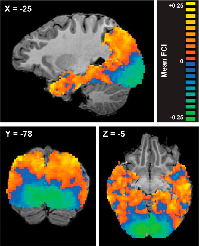
FCI derived from whole brain searchlight analyses: group mean FCI produced by a searchlight MVPA assessing conjunction- vs. feature-coding throughout visual cortex. A sphere of radius 5 functional voxels was swept through the imaged volume, constrained by a subject-specific gray matter mask encompassing occipital, temporal, and posterior parietal cortex. Taking each voxel in turn as the centroid of a spherical ROI, the feature and object classifiers were trained and their accuracies combined to produce a FCI that was entered into the map at the location of the centroid voxel. Orange indicates positive FCI (conjunction-coding); blue indicates negative FCI (feature-coding). Centroid voxels for which classifier performance did not exceed chance, as determined by a binomial test, were removed from individual subject maps (see materials and methods). FCI maps were constructed for each subject and scan session individually (see Fig. 5), then spatially smoothed with a Gaussian kernel (FWHM = 2 functional voxels). Smoothed maps were averaged across 2 sessions for each subject and across subjects. Scale is truncated at ±0.25 for optimal visualization of the data; some voxels possess FCI values >greater than +0.25 or less than −0.25.

Group-level statistical tests on searchlight data.

To find cortical locations of reliably nonzero FCI values—either positive indicating conjunction-coding or negative indicating feature-coding—we performed a group-level t-test at each voxel in the searchlight analysis, comparing the group mean FCI to zero. To do so, we took FCI maps from individual subjects and sessions that had been spatially smoothed with a Gaussian kernel with FWHM of two functional voxels and averaged over the two sessions for each subject, as described above. We tested only voxels that were associated with numeric FCI values for all eight subjects (i.e., voxels that did not contain an empty value after spatial smoothing, owing to disqualification during the screening process). We used an FDR-corrected α level of 0.05 (2-tailed) against a t-distribution with 7 degrees of freedom. Anatomical labels for identified sites in cortex were derived from the Automated Talairach Atlas available at www.talairach.org (Lancaster et al. 2000).

Quantifying the transition from feature- to conjunction-coding.

To quantify the transition from feature- to conjunction-coding along the ventral and dorsal pathways, we examined the FCI as a function of location along each pathway. To specify the location of a voxel in the ventral and dorsal pathways, we first defined three vectors in Talaraich coordinates: 1) a “Posterior Ventral” vector with its origin in the occipital pole (Tal co-ords, L: [−8 −101 −6]; R: [8 −101 −6]) extending to the center of LOC (Tal co-ords, L: [−44 −70 −4]; R: [43 −67 −4]); 2) an “Anterior Ventral” vector with its origin at the center of LOC, extending to the anterior tip of the temporal pole (Tal co-ords, L: [−35 28 −29]; R: [35 28 −29]); and 3) a “Dorsal” vector with its origin in inferior posterior occipital cortex (Tal co-ords L: [−10 −99 −14]; R: [10 −99 −14]) extending to the most superior/anterior point of the dorsal pathway contained in the scanned volume, in Brodmann area 7 (Tal co-ords L: [−14 −67 53]; R: [14 −67 53]). The goal was to project the Talairach coordinates of each voxel in the dorsal and ventral pathways onto the three vectors we defined, to produce a single, scalar metric specifying the location of each voxel along each pathway. To include only voxels in the appropriate cortical regions for each vector (e.g., to exclude anterior voxels from the Posterior Ventral vector and ventral voxels from the Dorsal vector), we defined a bounding box around each vector, outside of which voxels were excluded from the analysis (see Fig. 6). In all cases, the bounding box for each hemisphere terminated at X = 0 (the midline). For the Posterior Ventral vector, the boundaries of the box were X = 0 to X = the lateral extent of the Talairach bounding box; Y = −55 to the posterior extent of the Talairach bounding box; Z = 7 to Z =  the inferior extent of the Talairach bounding box. For the Anterior Ventral vector, the bounding box dimensions were X = 0 to X = the lateral extent of the Talairach bounding box; Y = −70 to the anterior extent of the Talairach bounding box; Z = 7 to Z = the inferior extent of the Talairach bounding box. For the Dorsal vector, the bounding box dimensions were X = 0 to X = the lateral extent of the Talairach bounding box; Y = −57 to the posterior extent of the Talairach bounding box; Z = −14 to the posterior extent of the Talairach bounding box. In addition, for the Posterior Ventral vector, we excluded any voxels with a scalar projection value beyond the end of the vector, which terminated at the center of LOC (i.e., any voxels within the bounding box located at a more extreme point along the vector than the center of LOC).

Fig. 6.

Quantification of the transition from feature- to conjunction-coding in the ventral and dorsal streams. Insets show the approximate extent and position of the 3 defined vectors Posterior Ventral, Anterior Ventral, and Dorsal in pink; the projection of a voxel location onto the vector to derive a scalar value for the voxel position in blue; and the bounding box defining the brain region included as part of each pathway in green (a subject-specific anatomical mask including only gray matter in occipital, temporal, and parietal lobes was also applied). Plots show the best-fitting regression lines relating the location of a voxel in each of the 3 pathways to the FCI for the spherical ROI surrounding the voxel. Each line shows 1 subject in 1 hemisphere; colors indicate different subjects; solid and dashed lines show left and right hemispheres, respectively. The far end point of the vector is more distant from occipital cortex (i.e., the vector is longer) for the Dorsal than the Posterior Ventral pathway; this may account for the higher FCI value at the vector end point in the Dorsal than the Posterior Ventral pathway, given that regression line slopes in the Dorsal and Posterior Ventral pathways were similar (x- and y-axes use the same scale for all 3 plots).

Having derived a metric specifying the location of each voxel in each of the three pathways, we plotted FCI values as a function of voxel location. FCI values were not spatially smoothed but were averaged over the two sessions for each voxel, within each subject. Separate plots were made for each subject and hemisphere, for each of the three defined pathways (Posterior Ventral, Anterior Ventral, and Dorsal). For each plot, we assessed the correlation between voxel location and FCI and found the best-fitting straight line describing the relationship by a least-squares method. The best-fitting straight lines for all subjects and hemispheres in all three pathways are shown in Fig. 6. We assessed differences in the slope of the best-fitting straight lines for the three pathways by performing a 2 × 3 repeated-measures ANOVA with factors Hemisphere (left, right) and pathway (Posterior Ventral, Anterior Ventral, Dorsal).

Evaluating the Properties of the Feature Conjunction Index with Synthetic Data

Construction of synthetic data.

To evaluate the FCI metric we created synthetic BOLD data sets. We used two different templates—feature-coded and conjunction-coded—to generate the signal that defined distinct patterns for the 16 stimuli in the set. In the feature-coded template, artificial voxels were switched “on” or “off” according to the presence or absence of a particular value of one of the four binary features, with all feature values represented by an equal number of voxels. In the conjunction-coded template, artificial voxels were switched “on” or “off” according to the presence or absence of a specific object stimulus from among the set of 16, with all objects represented by an equal number of voxels. All data sets possessed 256 voxels in total. We generated synthesized data sets in two ways: 1) by selecting a signal value from a range of magnitudes (between 0.01 and 0.5), applying this signal to “active” voxels according to the template, and superimposing this pattern of activation on top of a constant background of uniform random noise (range 0–1, standard deviation 0.289), resulting in two families of data sets (feature and conjunction coded) possessing signal-to-noise ratios (SNRs) ranging from 0.0012 to 3; and 2) by using a constant signal value of 1, applying this signal to “active” voxels according to the template, and superimposing this pattern on top of a background of uniform random noise whose amplitude was systematically manipulated (the range of the noise varied from a minimum range of 0–2, with standard deviation 0.5774, to a maximum range of 0–30, with standard deviation 8.66), resulting in two families of data sets (feature and conjunction coded) that possessed SNRs ranging from 0.0133 to 3. For both data synthesizing methods, data were normalized on a “per run” basis exactly as empirical BOLD data were normalized before analysis (grouping “trials” into sets of 32 containing 2 presentations per stimulus—a single scanner run—and normalizing across all trials in a run for each voxel).

Assessment of FCI.

Our goals were 1) to assess the intuition that feature-coded activation patterns produce negative FCIs and conjunction-coded patterns produce positive FCIs, when classifier performance is above chance, and 2) to examine the extent to which qualitative or quantitative shifts in FCI are produced by varying levels of noise. Following procedures identical to those used for empirical BOLD data, taking 100 synthetic data sets from each template—feature coded and conjunction coded—we ran feature- and conjunction-level classifiers and computed FCI values from the classifier outputs. We then plotted FCI values and classifier accuracies against SNR, for both data templates. Critically, we aimed to evaluate the FCI metric against the results from data sets that produced classifier accuracies in line with the range of accuracies seen in our empirical data. This is important because FCI values necessarily tend to zero when both feature- and object-level classifiers either know nothing (below-chance performance) or have perfect knowledge (approaching 100% accuracy). We emphasize that in our empirical data classifier accuracies never approached ceiling, and below-chance classification accuracies always disqualified an ROI from inclusion in the assessment of FCI.

RESULTS

FCI Reflects the Relative Contribution of Feature- vs. Conjunction-Coding in a Cortical Region

As seen in Fig. 2, analyses of synthetic data constructed according to a feature code and a conjunction code yielded FCI values that confirmed the interpretation of FCI outlined in materials and methods. Focusing on the data points within the gray boxes (for which mean classifier accuracies fell within the range observed in ROI-based analyses of the empirical data), when FCI values from each set of 100 simulations were compared with zero with a one-sample t-test (α = 0.05), it was confirmed that all feature-coded data sets produced negative FCI values and all conjunction-coded data sets produced significantly positive FCI values. We emphasize two key features of these simulation results. First, positive FCI values were never produced by a feature-coded template, and negative FCIs were never produced by a conjunction-coded template. Second, for both templates, increasing noise tended to push the FCI toward zero, making it less negative for feature-coded data and less positive for conjunction-coded data. However, in these simulations, FCI values derived from above-chance, empirically plausible classifier accuracies were always statistically distinguishable from zero (i.e., significantly negative or positive). Taken together, the simulations demonstrate that a region containing only object-sensitive voxels cannot produce a negative FCI and a region containing only feature-sensitive voxels cannot produce a positive FCI, precluding qualitatively misleading results. When the FCI takes near-zero values, in the presence of above-chance classifier accuracy, this likely represents a transition zone containing some mixture of feature- and conjunction-sensitive voxels, such that neither coding type is dominant. In the presence of high noise levels zero FCIs are harder to interpret, because they may reflect noise rather than a balance of feature and conjunction-coding. It is for this reason that, in the empirical analyses (both ROI based and searchlight), we screened out any ROIs for which classifier accuracy did not exceed chance. Despite this caveat regarding near-zero FCIs, it is nonetheless instructive that, even at high noise levels, numerically positive FCIs never emerged from a feature code and numerically negative FCIs were never produced by a conjunction code. The simulations thus reinforce the a priori intuition that the FCI indicates whether the voxel-level population code is relatively dominated by a feature code (negative FCI) or a conjunction code (positive FCI).

An intuitive understanding of the pattern of FCI values derived from synthetic data can be gained by considering how individual voxel activations map onto category identities, for each underlying coding type and classifier type. All classifiers used a linear kernel. First, consider that for hypothetical activation patterns with zero noise, both feature and conjunction knowledge would be perfect regardless of the underlying code (feature based or conjunction based) and FCI values would be zero. However, empirical BOLD data contain noise, which produces incomplete knowledge. In the case of noisy feature-coded data, reliable information is present for some but not all of the features (i.e., noise obscures the signal in some but not all of the feature-sensitive voxels). Each feature classifier must map feature-sensitive voxels onto feature categories, but these mappings are independent for the different categories: different voxels carry the information for each category. Although some voxels’ signal is obscured, reducing the feature classification accuracy for the feature categories coded by those voxels, the feature categories for which reliable information is present can still be classified because mappings from the reliable voxels to feature categories are unaffected by noise in the unreliable voxels. In contrast, the conjunction classifier must map feature-sensitive voxels onto object categories, which requires combining information from all features; therefore all voxel-to-category mappings are affected by the loss of information in some voxels. Consequently, object classification accuracy drops further than feature classification accuracy, and FCI is negative. In the case of noisy conjunction-coded data, the reverse scenario applies. Since the conjunction classifier learns independent mappings of conjunction-sensitive voxels to object categories (separate voxels in each case), noise on some but not all voxels reduces accuracy for some but not all categories. In contrast, the feature classifier must perform combinatorial mappings of conjunction-sensitive voxels onto feature categories, so the presence of noise on some voxels affects all voxel-to-feature category mappings. Hence, noise affects feature classifier accuracy more than conjunction classifier accuracy, producing positive FCI values.

What does this imply for the nature of the neural code? Positive FCIs are taken as indicating conjunction-coded activation patterns. In our simulations, this amounted to voxels in which the signal varied with the presence or absence of an object, without regard to its component features. That is, the intersection of the features comprising the object created a wholly new pattern, distinct from the pattern due to other objects sharing some of those features. A conjunction code is thus a nonlinear combination of features for which the whole is greater than the sum of the parts.

Transition from Feature- to Conjunction-Coding in Occipito-Temporal Cortex

We investigated whether early visual cortex employs feature-coding or conjunction-coding, and whether one scheme transitions to the other with progression toward the temporal lobe, by examining FCI in a series of functionally or anatomically defined ROIs: V1, V2, V3, and LOC. Taking stimulus-evoked activation patterns from across each ROI, we trained the classifiers using hold-one-out cross-validation and computed FCI for each subject and session separately (Fig. 3; Table 4). FCI differed significantly across ROIs [F(5,35) = 15.78, P < 0.001, η² = 0.693] but not across sessions [F(1,7) = 0.004, P = 0.95, η² = 0.001], with no interaction between Scan Session and ROI [F(5,35) = 0.133, P = 0.984, η² = 0.019]. Ordering the ROIs as [V1, V2v, V2d, V3v, V3d, LOC] revealed a significant linear trend [F(1,7) = 37.34, P < 0.001; η² = 0.842], suggestive of a transition from feature-coding toward conjunction-coding along early stages of the visual pathway. Regions V1 through V3 exhibited negative FCIs indicative of feature code dominance, while LOC revealed a numerically positive FCI that was significantly greater than in all other ROIs (revealed by nonoverlapping 95% CIs; Table 4). In our analysis of synthetic data, neither purely feature-based nor purely conjunction-based data (at SNR levels that yielded classifier accuracy within the range observed in the empirical ROI-based analyses) produced zero FCIs. We therefore interpret the near-zero, numerically positive FCI for LOC in terms of a hybrid code that contains both feature- and conjunction-coding, in contrast to the strong feature-coding detected in early visual cortex. In favor of this interpretation, we note two points. First, both feature and object classifier accuracy exceeded chance in LOC (see Tables 2 and 3). Given this above-chance classifier performance, and the simulation results reported above, it would not be possible to derive a numerically positive FCI if the true underlying code in LOC were as strongly feature based as in regions V1 through V3 (indicated by their very negative FCI values). Second, region LOC showed a significantly positive FMI for the midlevel conjunction of global shape (reported below), indicating that the quality of BOLD in LOC, in this data set, is sufficient to produce nonzero indexes when the information present in the activation patterns warrants such values.

Fig. 3.

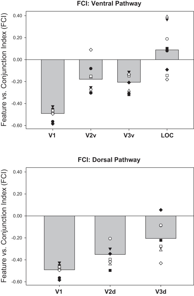
Feature conjunction indexes (FCIs) derived from ROI-based analyses: mean FCI (averaged over 2 sessions in each subject) for ROIs in early ventral visual stream (V1, V2v, V3v, LOC, top) and early dorsal stream (V1, V2d V3d, bottom). V1 is duplicated in top and bottom plots for ease of comparison. FCI is the natural logarithm of the ratio of object classifier accuracy to the product of the 4 feature classifier accuracies (see Fig. 1 and materials and methods). Positive FCI reflects conjunction-coding; negative FCI reflects feature-coding. Gray bars show group mean; plotted points show individual subjects, where each unique marker corresponds to the same individual subject across ROIs. See Table 4 for bootstrapped 95% confidence intervals (CIs) around the means. n = 8 subjects, 2 scan sessions each.

Feature- and Conjunction-Coding Throughout Visual Cortex

To assess feature- and conjunction-coding in cortical representations of objects beyond region LOC, and in the dorsal visual pathway, we examined all of visual cortex, using a searchlight approach (Kriegeskorte et al. 2006). At each spherical ROI, we performed classifier analyses (using hold-one-out cross-validation and screening out spheres in which classifier accuracy did not exceed chance) and computed the FCI, mapping the FCI value back to the centroid voxel of the sphere. In the group-averaged FCI map (Fig. 4), occipital regions exhibit the most negative FCIs indicative of feature-coding. With progression into regions anterior and superior to the occipital pole, the FCI first becomes less negative—suggesting a transition or “hybrid” region—and then becomes positive in occipito-temporal and posterior parietal regions, indicating the emergence of conjunction-coding in both ventral and dorsal pathways. Examination of FCI maps in individual subjects revealed the same pattern in every subject in both sessions: strongly negative FCIs in occipital regions with a transition to positive FCIs toward temporal and parietal regions (Fig. 5).

Fig. 5.

Individual subject FCI maps: raw FCI values plotted separately for the 2 scans (1, 2) in 3 individual subjects (G, H, and N). The 2 left columns correspond to the first scan, and the 2 right columns correspond to the second scan; each row depicts an individual subject. Color of a voxel indicates FCI for the spherical ROI surrounding it. Absence of color indicates the voxel was screened out because 1) it was not included in the anatomical (gray matter) mask, 2) the sphere surrounding the voxel contained too few voxels, or 3) accuracy for none of the classifiers exceeded threshold. There are many more absent voxels here than in the group mean FCI map (Fig. 4) because the spatial smoothing and averaging used in creating the group mean map eliminated many absent voxels. Scale is truncated at ±0.5 for optimal visualization; some voxels possess FCI values greater than +0.5 or less than −0.5. The scale differs from that of Fig. 4 because data within individual maps span a greater range.

Quantifying the Transition from Feature- to Conjunction-Coding

Next, we sought to quantify the relationship between cortical location and FCI in both ventral and dorsal pathways. To do so, we devised a metric to specify the location of the voxels in each pathway by defining three vectors in Talaraich coordinates: a Posterior Ventral vector with its origin in the occipital pole extending to the center of LOC; an Anterior Ventral vector with its origin in LOC extending to the anterior tip of the temporal pole; and a Dorsal vector with its origin in inferior posterior occipital cortex extending to the most superior/anterior point of the dorsal pathway in the scanned volume (in Brodmann area 7). For each vector we defined a bounding box around the vector to constrain the anatomical region from which voxels were drawn (Fig. 6) and projected the Talairach coordinates of voxels within the box onto the vector, yielding a scalar value for each voxel that specified its location along the vector. Finally, for each subject, for all three vectors in each hemisphere separately, we computed 1) the correlation between the location of a voxel and the FCI of the spherical ROI centered on that voxel and 2) the slope of the best-fitting regression line relating voxel location to FCI (Fig. 6). The correlation between location and FCI was positive and highly significant in all eight subjects in both hemispheres for the Dorsal vector (P < 0.0001) and the Posterior Ventral vector (P < 0.01), reflecting a robust transition from feature-coding at the occipital pole to representations more dominated by conjunction-coding in lateral occipital and superior parietal cortices, respectively. For the Anterior Ventral vector, the correlation was positive and significant (P < 0.01) in both hemispheres for five of eight subjects; in one subject (yellow in Fig. 6) the left hemisphere was negatively correlated (a decrease in FCI with anterior progression; P < 0.05) and the right was positively correlated (P < 0.001); in the two remaining subjects (black and magenta in Fig. 6), the left hemisphere was significantly negatively correlated (P < 0.0001) and the right was not correlated (P > 0.2). The slopes of the best-fitting regression lines differed for the three vectors [F(2,14) = 23.71, P < 0.001] but did not differ by hemisphere [F(1,7) = 0.026, P = 0.877], with no hemisphere × vector interaction [F(2,14) = 2.889, P = 0.089]. Slopes for the Anterior Ventral vector were smaller than for the Posterior Ventral (P < 0.001) and Dorsal (P < 0.0001) vectors, which did not differ from each other (P = 0.62). These results suggest that, for the present stimulus set, the greatest transition from feature-coding to conjunction-coding occurs in posterior regions, in both ventral and dorsal pathways. A possible reason for the shallower transition toward conjunction-coding in the anterior ventral pathway is that the object-level conjunctions comprising these simple, novel objects may be fully specified in relatively posterior sites, just beyond the occipito-temporal junction (Figs. 4 and 7). Indeed, the stimuli with which Erez et al. (2016) revealed conjunction-coding in anterior temporal regions were three-dimensional, colored objects that likely better engaged anterior visual regions.

Fig. 7.

Cortical sites of feature- and conjunction-coding observed at the group level. Statistical map shows the results of a t-test at each voxel comparing the group mean FCI value associated with the spherical ROI surrounding that voxel to zero. The map was thresholded at P = 0.05, 2-tailed (FDR corrected for multiple comparisons). Blue voxels possess FCI values significantly less than zero (feature-coding); orange voxels possess FCI values significantly greater than zero (conjunction-coding). All but 1 voxel with statistically reliable negative FCI values were located in occipital cortex, whereas all voxels with statistically reliable positive FCI values were located anterior or superior to the occipital feature-coding regions. Voxels exhibiting significant conjunction-coding appeared in multiple sites bilaterally, including posterior parietal lobe, fusiform gyrus, parahippocampal gyrus (including left perirhinal cortex), hippocampus, and anterior temporal pole. Axial slices are radiologically flipped (left hemisphere appears on right). In sagittal slices, positive X coordinates indicate right hemisphere.

Cortical Sites of Extreme Feature- and Conjunction-Coding

Finally, to search for cortical sites demonstrating statistically reliable extremes of feature- or conjunction-coding, we compared the group mean FCI at each voxel to zero (2-tailed t-test, FDR corrected; positive t-values indicate conjunction-coding, and negative t-values feature-coding). This analysis assumes anatomical and functional correspondence of points in Talairach space across subjects; it is therefore conservative, particularly for conjunction-coding, the cortical sites of which are likely more widely and variably distributed across subjects. Nonetheless, we revealed a large occipital region of feature-coding along with multiple conjunction-coding sites throughout occipito-temporal, ventral temporal, and parietal cortices, extending into the parahippocampal gyrus, medial temporal lobe, and anterior temporal pole (Fig. 7). We note the lower prevalence of above-threshold voxels contributing to each subject’s FCI map in regions toward the anterior temporal lobes (see Fig. 5), and we therefore interpret our findings in these regions with caution; in contrast, data in the occipital, posterior temporal, and posterior parietal lobes were much less sparse, and so findings in these regions can be interpreted with greater confidence. Most important is the overall pattern at the group level: in line with a feature-to-conjunction transition hypothesis, all conjunction-coding sites were located anterior or superior to the feature-coding sites, which were confined to the occipital lobe (excepting a single more anterior feature-coding voxel at [10 −51 5], in the inferior posterior cingulate).

No Effect of Visual Search Training on Feature- or Conjunction-Coding as Measured by FCI

We detected no effect of visual search training on the prevalence of feature- vs. conjunction-coding, as measured by the FCI, in participants’ cortical activation patterns. As reported above, there was no main effect of Session and no Session × ROI interaction on the critical FCI measure (where Session is the factor partitioning data collected before vs. after visual search training). Because the visual search task required object individuation, any observed change in neural representations was expected to increase conjunction-coding. There are several possible explanations for the absence of an observed training effect on the neural representations. First, in our training procedure, daily sessions were terminated for each subject when the RT-set size slope appeared to be approaching an asymptotically low value (mean 11.1 days; range 7–15 days). This relatively short training duration may have been insufficient to produce full unitization of the conjunctive stimuli, a notion in line with the fact that RT-set size slopes were still significantly positive in the final training session (Table 6). Second, the stimuli were perceptually simple and devoid of semantics, and the task did not involve naming; thus our training may have failed to engage the learning mechanisms known to influence neural representations in visual cortex for richer, more meaningful objects (e.g., Folstein et al. 2013; Gauthier et al. 1999). A third possibility is that cortical representations did change with training, but the data were too noisy to allow detection of these changes at the individual subject level and the sites at which changes occurred varied in location across participants, obscuring findings at the group level.

Table 6.

Behavioral performance during training on conjunctive visual search task

	Accuracy on Final Session	RT-Set Size Slope First Session, ms/item	RT-Set Size Slope Final Session, ms/item
Mean (±SE)	0.893 (±0.020)	297 (±37)	200 (±20)

Accuracy on the final session (and in all earlier sessions, not reported) far exceeded the chance performance level of 50%. RT-set size slopes decreased significantly from the first to the final session (P < 0.05) but were still significantly >0 in the final session (P < 0.0001). Shiffrin and Lightfoot (1997) trained subjects for many more sessions of conjunctive visual search (~50 days compared with 11.1 days in present study) and observed RT-set size slopes as low as 50 ms/item on the final session.

Coding of Midlevel Conjunctions

We examined the extent to which ROIs in the ventral and dorsal pathways coded for simple features vs. midlevel conjunctions (FMI; Fig. 8), and coded for midlevel conjunctions vs. whole object conjunctions (MCI; Fig. 9). We found the same trend as revealed by the FCI analysis: both FMI and MCI measures took negative values in posterior regions such as V1 (indicating that feature-coding dominates over midlevel conjunction-coding and midlevel conjunction-coding dominates over whole object conjunction-coding) but increased toward positive values in more anterior regions such as V3d and LOC.

Fig. 8.

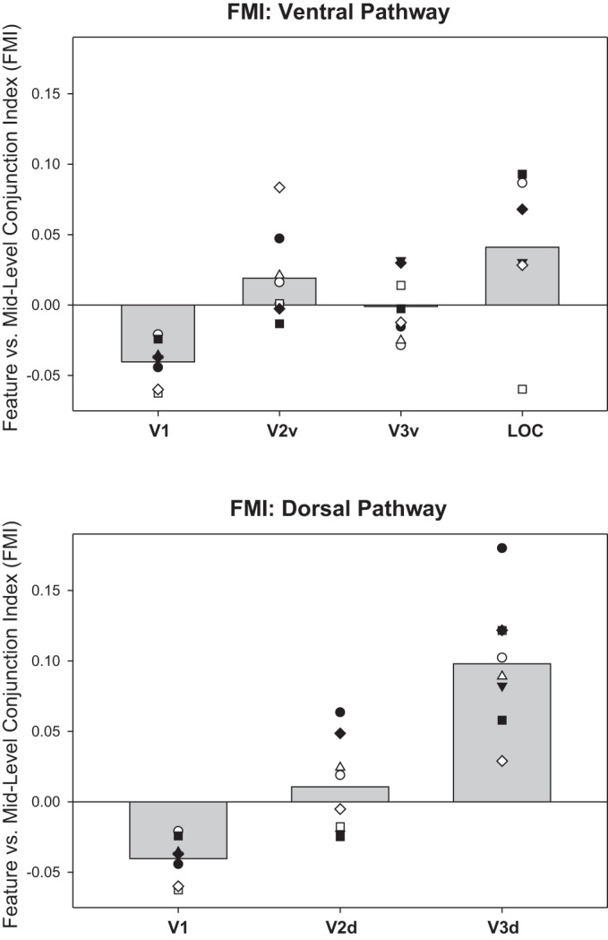
Feature vs. midlevel conjunction indexes (FMI) derived from ROI-based analyses: mean FMI (averaged over 2 sessions in each subject) for ROIs in early ventral visual stream (V1, V2v, V3v, LOC, top) and early dorsal stream (V1, V2d V3d, bottom). V1 is duplicated in top and bottom plots for ease of comparison. FMI is the natural logarithm of the ratio of the midlevel conjunction classifier accuracy to the product of the 2 feature classifier accuracies for the features defining that midlevel conjunction (see materials and methods). Positive FMI reflects a preference for coding midlevel conjunctions over features; negative FMI reflects the reverse preference. Gray bars show group mean; plotted points show individual subjects, where each unique marker corresponds to the same individual subject across ROIs.

Fig. 9.

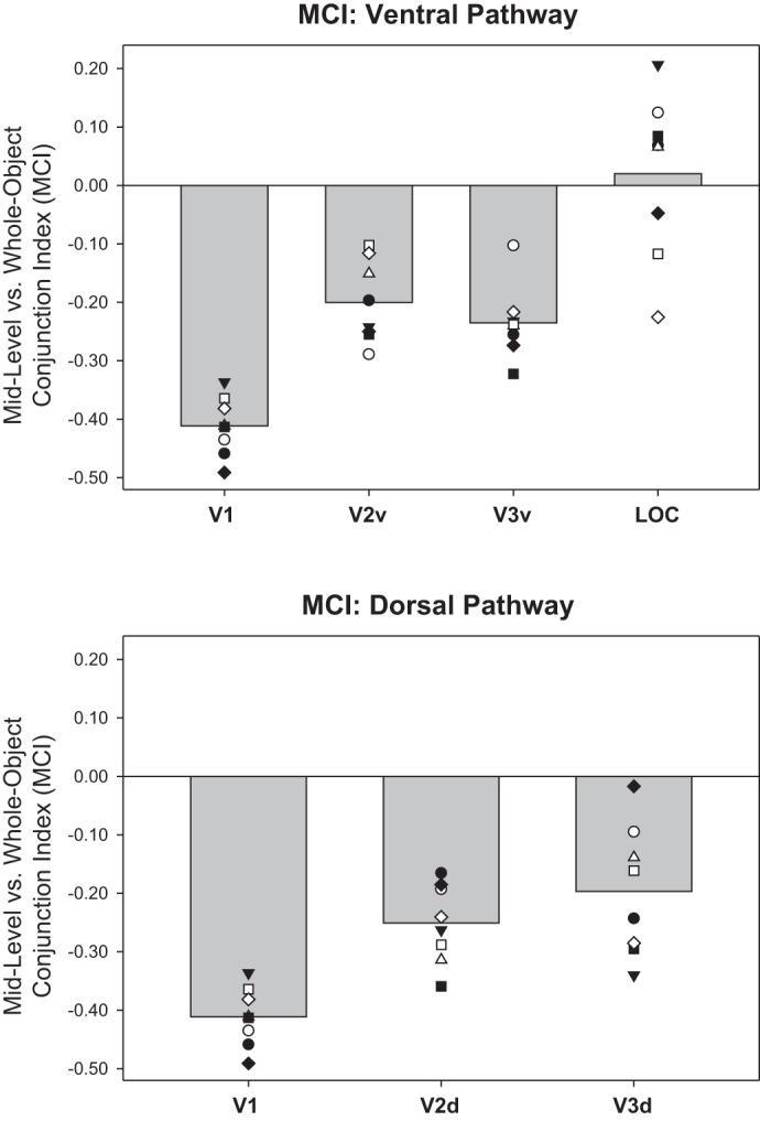
Midlevel conjunction vs. whole object conjunction indexes (MCI) derived from ROI-based analyses: mean MCI (averaged over 2 sessions in each subject) for ROIs in early ventral visual stream (V1, V2v, V3v, LOC, top) and early dorsal stream (V1, V2d V3d, bottom). V1 is duplicated in top and bottom plots for ease of comparison. MCI is the natural logarithm of the ratio of the whole object classifier accuracy to the product of the accuracies of each pair of midlevel conjunction classifiers that define the whole object (see materials and methods). Positive MCI reflects a preference for coding whole objects over midlevel conjunctions; negative MCI reflects the reverse preference. Gray bars show group mean; plotted points show individual subjects, where each unique marker corresponds to the same individual subject across ROIs.

Statistical assessment of FMI by ANOVA excluded LOC because of missing cells. Specifically, screening (to remove any session-subject-ROI data point for which no classifier exceeded chance as determined by a binomial; see materials and methods) resulted in the removal of several data points in LOC only, such that midlevel conjunctions 1 and 3 were determined on the basis of six and seven subjects, respectively, and the mean over all conjunctions was determined on the basis of six subjects (i.e., only those individuals who contributed a data point for all 4 midlevel conjunctions). ANOVA performed on the remaining ROIs revealed that FMI differed significantly across ROIs [F(4,28) = 21.07, P < 0.001, η² = 0.751] and across sessions [F(1,7) = 11.96, P = 0.011, η² = 0.631], with no interaction between Scan Session and ROI [F(4,28) = 1.54, P = 0.219, η² = 0.180]. The small but significant difference across sessions was due to a decrease of 0.015 in FMI from the first to the second scan session, i.e., a change after visual search training toward feature-coding and away from midlevel conjunction-coding. Since visual search training focused on the unique identity of the whole object, it is not clear what should have been expected for any shift in neural coding of midlevel conjunctions. This shift toward more negative FMIs might result from increased attention to individual features over midlevel conjunctions after training, but the shift was small in magnitude.

Statistical assessment of MCI by ANOVA revealed that MCI differed significantly across ROIs [F(5,35) = 17.79, P < 0.001, η² = 0.718] but not across sessions [F(1,7) = 0.026, P = 0.876, η² = 0.004], with no interaction between Session and ROI [F(5,35) = 0.72, P = 0.613, η² = 0.093].

Together, the FMI and MCI results yield three notable insights. First, the FMI analysis demonstrates that when simple conjunctions (rather than whole object conjunctions) are pitted against the basic features, the zero point of the transition from feature-coding to conjunction-coding occurs earlier in both visual pathways, near area V2. Second, the combination of FMI and MCI results for area V3d suggests that it codes primarily for midlevel conjunctions in the present stimulus set: in V3d, the FMI (features vs. midlevel conjunctions) was significantly positive (1-sample t-test compared with zero, P < 0.001) whereas the MCI (midlevel vs. whole object conjunctions) was significantly negative (1-sample t-test, P = 0.0016), suggesting that midlevel conjunction-coding dominates over both feature-coding and whole object conjunction-coding. Third, the FMI values for area LOC suggest that the extent to which this region codes for conjunctions relies heavily upon its coding of shape. As seen in Table 7, which shows FMI values for individual midlevel conjunctions, LOC yielded a significantly positive value only in the case of conjunction 1—the combination of Left and Right outlines corresponding to the global form of the stimulus (t-test, P = 0.0019). (We note that, even though the contour features each possess their own “global” shape, a positive FMI value for conjunction 1 nonetheless indicates that the brain region codes for the intersection of the two contour features. If the activation patterns comprised only a linear combination of the separate representations of each contour feature, the conjunction classifier would show no performance advantage over the feature classifiers.) In contrast, for conjunction 2 (the combination of 2 spatial frequencies, or “texture”), LOC yielded a significantly negative FMI (t-test, P = 0.0388) indicative of dominant feature-coding.

Table 7.

Feature midlevel conjunction index for the four plausible midlevel conjunctions separately

	Ventral Stream				Dorsal Stream
	V1	V2v	V3v	LOC	V2d	V3d
Midlevel conjunction 1 (Global Shape)	0.0005 (±0.026)	−0.0419 (±0.039)	−0.044 (±0.035)	0.181 (±0.038)	0.056 (±0.031)	0.195 (±0.060)
Midlevel conjunction 2 (Texture)	−0.089 (±0.024)	0.117 (±0.028)	0.086 (±0.035)	−0.095 (±0.036)	−0.037 (±0.027)	−0.003 (±0.048)
Midlevel conjunction 3 (Right Component)	0.076 (±0.017)	0.0029 (±0.028)	−0.108 (±0.024)	0.116 (±0.063)	0.157 (±0.023)	0.090 (±0.035)
Midlevel conjunction 4 (Left Component)	−0.148 (±0.026)	−0.0016 (±0.024)	0.061 (±0.024)	−0.044 (±0.053)	−0.134 (±0.021)	0.110 (±0.049)
Overall mean FMI	−0.040 (±0.005)	0.019 (±0.011)	−0.001 (±0.008)	0.041 (±0.023)	0.011 (±0.012)	0.098 (±0.016)

Values are mean (±SE) FMI for each midlevel conjunction separately, by ROI, across subjects. Mean values over all 4 midlevel conjunctions for each ROI are also shown in Fig. 8. Data were averaged over 2 sessions for each subject.

DISCUSSION

Several recent fMRI studies have examined conjunction-coding in humans (Baeck et al. 2013; Baumgartner et al. 2013; Erez et al. 2016; MacEvoy and Epstein 2009; Pollmann et al. 2014; Seymour et al. 2009, 2010; van den Honert et al. 2017; Zhang et al. 2015). Two of these studies revealed conjunction-coding for combinations of static, abstract features (e.g., color, form) into visual objects, in the ventral pathway (Erez et al. 2016; Seymour et al. 2010). However, neither study was able to definitively rule out an explanation of the observed conjunction code in terms of feature-coding combined with saturation of the BOLD signal; that is, because both studies presented the critical conjunctions by temporally interleaving subsets of features that comprise the conjunction, rather than by presenting the whole conjunction simultaneously, the presence of neurovascular nonlinearities (i.e., saturation of BOLD) for some features more than others may have given the appearance of a conjunction code even in feature-coding voxels. Two further studies in this set (Baumgartner et al. 2013; Pollmann et al. 2014) used a method more similar to ours, measuring whether classification accuracy for two feature dimensions together was superadditive compared with the classification of each dimension alone. However—perhaps related to the use of multiple-object stimulus displays and a visual search task—these studies revealed conjunction-coding only in parietal regions. Moreover, no study of object processing that we know of has explicitly investigated the complement to conjunction-coding, namely, feature-coding—that is, the extent to which neural representations are more informative about individual features than conjunctions of those features (but see van den Honert et al. 2017 for a slightly different definition of feature-based representations in a study of scene-level conjunctions). Without directly comparable measures of feature-coding and conjunction-coding, the evidence for a transition from one to the other cannot be assessed. Therefore, three important questions remain unresolved: Is there evidence for a conjunction-based object code in the human ventral visual stream, when an explanation in terms of BOLD signal saturation is ruled out? If the answer is yes, is conjunction-coding dominant even early in the ventral stream or does it emerge along the pathway? If it emerges, at what point does the transition from feature- to conjunction-coding occur?

To answer these questions, we measured the relative dominance of feature- vs. conjunction-coding throughout visual cortex by directly comparing evidence for the two coding schemes in each cortical region. Critically, evidence for both schemes was derived from a common neuroimaging data set acquired while participants viewed systematically constructed conjunctive visual stimuli. We revealed a transition from feature-dominated to conjunction-dominated coding, with progression from primary visual cortex into temporal cortex (Figs. 3, 4, and 6). This provides the first direct evidence in humans for an object representation scheme in the ventral pathway that is characterized by a transition from feature- to conjunction-coding. Strikingly, the same shift from feature- to conjunction-coding was evident in the dorsal pathway, where it was as steep and robust as in the posterior ventral pathway (Figs. 3 and 6).

The results are incompatible with a global feature-coding hypothesis, which predicts the feature-coding we observed in early regions but not the conjunction-coding that we saw in both parietal and anterior ventral sites (Fig. 7). Similarly, the results are incompatible with a global conjunction-coding hypothesis, which predicts the conjunction-coding seen in downstream sites but cannot accommodate the findings in V1, where—regardless of whether feature-coding was compared with the coding of midlevel conjunctions (FMI) or whole conjunctions (FCI)—the index was always negative, reflecting more information about features than about the conjunctions of those features (Figs. 8 and 3). Thus the explicit measurement of feature-coding via negative FCI values was critical to distinguishing between the alternative theoretical accounts.

We revealed significant conjunction-coding in a range of sites bilaterally, including posterior parietal cortex, fusiform and parahippocampal gyri, medial temporal lobes, and anterior temporal poles (Fig. 7). These findings concur with prior reports of conjunction-coding throughout the ventral visual stream and perirhinal cortex (Erez et al. 2016) and in parietal lobe (Baumgartner et al. 2013; Pollmann et al. 2014). In addition, we provided a systematic investigation of feature-coding across human visual cortex, revealing significant selectivity for features over conjunctions in retinotopically defined V1 (Figs. 8 and 9) and across posterior occipital regions more generally (Fig. 7). For the present stimulus set, the transition from feature-coding to conjunction-coding—the zero point of the FCI—occurred in the ventral pathway near the occipito-temporal junction and in the dorsal pathway at approximately the superior border between Brodmann areas 18 and 19 of the occipital lobe (Fig. 4).

We also examined coding for intermediate-complexity stimulus components, by pitting features against midlevel conjunctions (in the FMI) and midlevel conjunctions against whole object conjunctions (in the MCI). These measures suggested that the transition from feature- to conjunction-coding occurs earlier in the visual pathway for simpler conjunctions, that V3d may preferentially code for midlevel conjunctions, and that conjunction-coding in LOC may be driven by coding of shape, or global form, in line with prior reports (Drucker and Aguirre 2009; Malach et al. 1995; Ostwald et al. 2008). The midlevel conjunction findings also corroborated our interpretation of the main FCI measure, as discussed below.

Transition from Feature- to Conjunction-Coding: Gradual or Abrupt?

Because feature-coding dominates in V1 and conjunction-coding sites exist in fusiform gyrus and posterior parietal lobe (Fig. 7), we can conclude that somewhere between early visual areas and later stages of both the ventral and dorsal pathways a transition from feature- to conjunction-coding occurs. Figures 4, 5 (whole brain analyses), and 6 (correlation analysis) imply a gradual transition. However, it is not possible to conclude definitively from the FCI that the transition from feature- to conjunction-coding in the brain is gradual rather than abrupt. A graded change in the FCI is somewhat guaranteed for the whole brain, searchlight analyses by the spatially overlapping spherical ROIs and for the correlations by the assumed linear relationship between FCI and voxel location. We note that this guarantee does not apply to the ROI results in Fig. 3, which reflect the same gradual transition, because we did not perform any spatial averaging of the data in this analysis. However, even in this case, it is possible that a reduction in SNR from V1 toward higher visual regions (V3, LOC) induced FCI values to increase toward zero, without an underlying gradual shift from feature-coded toward conjunction-coded representations (see simulations, Fig. 2). Thus it may be that the cortical code shifts abruptly from feature to conjunction based somewhere between V3 and IT, and the appearance of a gradual transition from V1 through LOC is caused by increasing noise. However, we think this unlikely given the FMI values that were derived from the same BOLD data (Fig. 8). Specifically, the FMI increased from negative values in V1, through zero in V2, to positive values in V3d. That is, for simpler conjunctions a similarly gradual transition in coding occurs across the same brain regions, but the steady increase in FMI values does not stop at zero (as it would if driven by noise alone) but instead pushes through to positive, conjunction-coding values in V3d. Thus for FMI an explanation involving increasing noise with progression up the pathway cannot explain the pattern of results.

Conjunction-Coding in the Dorsal Pathway

The emergence of conjunction-coding in the dorsal pathway was perhaps more unexpected than in the ventral pathway. However, this finding aligns well both with the documented role of parietal cortex in feature binding (Ashbridge et al. 1997; Cohen and Rafal 1991; Friedman-Hill et al. 1995; Humphreys et al. 2000; Muggleton et al. 2008) and with recent claims that the role of the dorsal stream in vision extends beyond spatial processing or attentional binding. That is, our observation of object-specific coding in parietal cortex—elicited while participants discriminated highly similar visual objects—suggests that the dorsal pathway constructs content-rich, hierarchical representations containing information that is critical for object identification, in parallel with the ventral stream (Jeong and Xu 2016; Konen and Kastner 2008). Given that feedback from parietal cortex has been shown to shape visual representations in the ventral processing pathway (e.g., Hopfinger et al. 2000; Parks et al. 2015; Rowe et al. 2005), it is possible that interactions between dorsal and ventral regions increased the similarity of representations across the two streams.

V2: Coding of Features and Simple Conjunctions

The negative FCI recorded for V2 suggests feature-coding (Fig. 3), which might appear to contradict previous reports of conjunction-coding in this region for stimuli comprising combinations of simple features (Anzai et al. 2007; Seymour et al. 2010). However, negative FCI values in V2 do not rule out the existence of conjunction-based information altogether; they merely imply that any conjunction code is relatively swamped by a stronger feature code. Moreover, the complementary FMI metric that assesses coding of simpler conjunctions—similar in complexity to the stimuli of Anzai et al. and Seymour et al.—revealed near-zero (numerically positive) scores in V2. These FMI values imply an intermediate code in V2 that includes a substantial subset of voxels sensitive to midlevel components. A strength of the present method, whether used to compare features with midlevel conjunctions (FMI) or with whole object conjunctions (FCI), is that it reveals the relative dominance of feature-based vs. conjunction-based information in each case, rather than simply detecting the presence or absence of only one type of information.

Interpreting the FCI

An analysis of synthetic data supported our interpretations of the FCI metric (Fig. 2). Across a range of SNR values for which classifier performance was within the range observed in empirical ROIs (and thus, also, above chance), negative FCIs were produced only by synthetic feature-coded data and positive FCIs emerged only from synthetic conjunction-coded data. These properties held true whether we synthesized data by holding noise constant and manipulating signal strength or by holding signal constant and manipulating noise. Thus the sign of the FCI reliably indicates the relative dominance of feature- vs. conjunction-coding, and varying noise levels do not produce distortions in the FCI that lead to qualitatively erroneous conclusions. Accordingly, the method mitigates somewhat against the problem of varying noise levels that has complicated prior attempts to use fMRI to compare the neural code across diverse brain regions. For example, if a standard MVPA method detects greater classification accuracy for simple visual features in early visual cortex than in later visual regions, this could be because the neural representations in early visual regions exhibit stronger feature-coding or because early visual cortex, situated peripherally, produces a BOLD signal with greater SNR. In the present method, because the feature- and conjunction-coding measures are placed in a ratio, and both measures are affected by the noise in each cortical region, the relative dominance of feature- vs. conjunction-coding in a region maps consistently to negative vs. positive FCI values in the face of varying noise.

In sum, the simulations demonstrate that the FCI can be used to determine which regions exhibit feature- vs. conjunction-coding and approximately localize the region in cortex where the code transitions from one to the other, for a given stimulus set.

Potential Influence of Sensitivity to Midlevel Conjunctions on the FCI

Because the binary features used in our data set included two shape outlines and two spatial frequencies, the intersection of any two of these features created incidental, novel shapes and textures that correspond to “midlevel conjunctions” like those we decoded for entering into the FMI and MCI (for example, in Fig. 1D: the global outline shared by stimuli 1, 3, 9, and 11 or the central texture shared by stimuli 1, 2, 5, and 6). Consider a brain region containing voxels sensitive to these midlevel conjunctions, rather than to the binary features or the whole object (4 featured) conjunctions on which classifiers are trained to generate the FCI: would this spuriously bias FCI toward either positive or negative values? For the whole object conjunction classifier, when voxels possess reliable information about just one of these midlevel conjunctions, the 16-way problem is reduced to a 4-way problem, facilitating above-chance classification and inflating the FCI toward more positive values. However, the feature classifiers would also benefit from midlevel conjunction-coding voxels: reliable information about one midlevel conjunction fully specifies two of the four binary features when classifying any of the 4 stimuli that possess that midlevel conjunction and provides a heuristic for classifying the other 12 stimuli that do not possess that midlevel conjunction (namely, “predict the feature values not included in the midlevel conjunction”) that is neutral for 8 of those stimuli and helpful for the other 4. On average across all stimuli, feature classification performance would be boosted by midlevel conjunction-coding voxels, reducing the FCI toward more negative values. The net effect, across both classifier types and all stimuli, is that midlevel conjunction-sensitive voxels in an ROI should boost feature- and conjunction-classifier performance equally, pushing any nonzero FCI, either negative or positive, toward zero.

Multiple Possible Routes to a Hybrid Code

We suggested earlier that zero FCI (in the presence of above-chance classifier accuracy) might be produced by hybrid-coded activation patterns, a mixture of feature-sensitive and whole object-sensitive voxels. However, given the presence of midlevel conjunctions in the stimuli it is equally possible that zero FCI is produced by voxels sensitive to those midlevel conjunctions. Importantly, this alternative interpretation of a zero FCI is still in keeping with the spirit of the measure: whether a cortical region exhibits zero FCI because of a heterogeneous mix of feature- and conjunction-coding voxels or because of midlevel conjunction-coding, that coding scheme should be considered intermediate, lying between strongly feature-coded and strongly whole object-coded representations. In line with the idea that sensitivity to midlevel conjunctions tends to yield FCIs close to zero, whole brain analyses revealed that the zero point in FCI lies near area LOC—known to represent global shape (Drucker and Aguirre 2009; Malach et al. 1995; Ostwald et al. 2008)—and area V4—known to exhibit texture-selective responses (Arcizet et al. 2008; Dumoulin and Hess 2007; Hanazawa and Komatsu 2001). Global shape and texture constitute midlevel conjunctions in the present stimulus set.

A further possibility is that a hybrid code, comprising a mixture of feature- and conjunction-sensitive responses, is generated not by combining spatially adjacent voxels of each type within an ROI but rather by combining temporally adjacent responses of each type within the same neurons. Connor and colleagues (Brincat and Connor 2006; Yau et al. 2013) recorded activation in monkey visual cortex and reported a dynamic neural code that evolved over time. Immediately after stimulus onset neurons in pIT and V4 were tuned to simple features, but ~50–60 ms later the same neurons responded nonlinearly to multipart configurations of those features (simple orientations were combined into multiorientation curves in V4 and simple curved contour fragments into multipart configurations in pIT). Because the BOLD signal has insufficient temporal resolution to distinguish between response types that evolve on the order of milliseconds, we cannot determine whether the hybrid code we observed was generated by a transition from feature- to conjunction-coding over time, but it is interesting that the areas producing zero FCI values in our data (occipito-temporal regions) lie near the regions identified in these electrophysiological studies (pIT and V4).

Changes in Receptive Field Size with the Emergence of Conjunction-Coding

The emergence of conjunction-coding in the ventral and dorsal pathways is accompanied by a systematic change in another property—RF size. This is relevant to measuring feature- and conjunction-coding with our stimulus set, because the total stimulus area containing conjunction information is smaller than the area containing information about features. If larger RFs (which capture the whole stimulus) capture conjunction and feature information to a similar extent, whereas smaller RFs (which capture small stimulus subsections) capture relatively more feature information on average, does this bias small-RF brain regions toward feature-coding? Even with a small RF it is possible to capture conjunction information in this stimulus set, since each stimulus contains numerous points of intersection of the two outlines and fill patterns that uniquely define the stimulus. Moreover, even neurons with RFs in peripheral regions might code conjunction information through collateral interactions or feedback from higher regions, such that the feature information across a combination of neurons is pooled to construct the conjunction. So, in regions with small RFs there is not a total absence of neurons that capture conjunction information, just a greater number of neurons able to capture feature information. Thus the question of whether the greater spatial extent of feature than conjunction information in the stimuli biases regions with small RFs toward feature-coding rests upon whether the conjunction classifier in such a region is impeded by receiving inputs from a large number of voxels that code nondiagnostic information (features) along with inputs of diagnostic information (conjunctions). Empirically, it is not always the case that including less informative voxels in an ROI causes classifier performance to drop, relative to when a smaller subset of more informative voxels are used (e.g., Filimon et al. 2015).

In addition, although increasing RF size could be described as a potential confound that shifts the balance of coding toward conjunctions in higher cortical areas, this “confound” may in fact be part of the (adaptively evolved) brain mechanism by which conjunction-coding emerges in higher regions. In other words, part of the function of large RF sizes may be to enable conjunction-coding. Real-world objects at real-world viewing distances are most often captured by the visual system at sizes that afford apprehension of the whole object by an IT neuron, and apprehension of only small subsections of the object by a neuron in V1, and this is likely not an accident of natural selection. Thus although an experimenter might seek to rule out any influence of RF size by presenting very small stimuli that are captured entirely by the RFs of V1 neurons, this scenario would not mimic natural viewing conditions. Moreover, the use of very small stimuli would introduce other systematic biases: small, centrally presented stimuli would be captured in V1 by only a small set of neurons with foveally located RFs but by almost all neurons in IT, so that the recorded activation data would exclude any contribution from peripheral RFs in early brain regions but not in later regions; and small stimuli might be rendered at such low resolution that the fine details of the conjunction are not perceived and stimuli are instead encoded as featurelike approximations in all brain regions.

Generalization to Coding for Other Visual Features and Their Conjunctions

We examined conjunctions of spatial frequency and contour. Spatial frequency is represented in V1 (Foster et al. 1985), whereas shape contour is represented in higher regions such as V4, pIT, and LOC (Brincat and Connor 2004, 2006; Drucker and Aguirre 2009; Yau et al. 2013). However, classification of our binary contour features was good in V1 and V2 (Table 2), implying that, given the small RF sizes, these regions represented the contour features in terms of small, local oriented segments. To what extent do these findings generalize to conjunctions of other features such as orientation, color, and motion? Orientation, like spatial frequency, is an elemental building block of vision, well represented in V1 (Hubel and Wiesel 1968). We suggest that shape is a visual attribute somewhat analogous to color and motion: for all three attributes, some information supporting classification is available in V1, but more holistic or categorical information emerges in higher regions—V4 for color (Brouwer and Heeger 2013) and V3 or V5/MT for motion (Gegenfurtner et al. 1997; Movshon et al. 1985). Thus the feature conjunctions we examined may be typical of the part-to-whole integration operations putatively performed across the visual hierarchy. In line with this, empirical results for other conjunction types are relatively consistent with the present findings: conjunction-coding for two-featured conjunctions (of complexity similar to our FMI) was reported in V2, V3, and parietal sites (Anzai et al. 2007; Baumgartner et al. 2013; Gegenfurtner et al. 1997; Pollmann et al. 2014). These prior studies did not examine feature-coding (as we define it) or the evidence for a transition from feature- to conjunction-coding. However, we tentatively suggest that the posterior-to-anterior transition we observed is likely to apply for conjunctions of many flavors, because electrophysiology studies point to this conclusion (Kobatake and Tanaka 1994; Rust and DiCarlo 2010, 2012). An important caveat is that we do not claim that specific, quantitative aspects of our results can be generalized, such as the cortical locations of the transition point and of conjunction-coding sites. Quantitative details are likely specific to each stimulus set, and the present study merely provides a tool for their investigation.

Conclusions

Our novel method permits the systematic investigation of feature- and conjunction-coding and may be applicable not just to vision but to other modalities such as audition or motor action (Lee et al. 2012; Wurm and Lingnau 2015). Within vision, the method will enable future investigation of a range of features not included in our stimulus set (including color, orientation, and motion), to examine how conjunction-coding emerges for different feature types and combinations. The present finding of a transition from feature- to conjunction-coding along both ventral and dorsal visual pathways has implications for theories of the functional architecture of visual object processing.

GRANTS

This work was funded by National Science Foundation (NSF) CAREER Award 1554871 to R. A. Cowell, by National Eye Institute Grant R01 EY-025872 to J. T. Serences, and by NSF Grant BCS-0843773.

DISCLOSURES

No conflicts of interest, financial or otherwise, are declared by the authors.

AUTHOR CONTRIBUTIONS

R.A.C. and J.T.S. conceived and designed research; R.A.C. performed experiments; R.A.C. and K.R.L. analyzed data; R.A.C., K.R.L., and J.T.S. interpreted results of experiments; R.A.C. prepared figures; R.A.C. drafted manuscript; R.A.C. and J.T.S. edited and revised manuscript; R.A.C., K.R.L., and J.T.S. approved final version of manuscript.

REFERENCES

- Anzai A, Peng X, Van Essen DC. Neurons in monkey visual area V2 encode combinations of orientations. Nat Neurosci 10: 1313–1321, 2007. doi: 10.1038/nn1975. [DOI] [PubMed] [Google Scholar]
- Arcizet F, Jouffrais C, Girard P. Natural textures classification in area V4 of the macaque monkey. Exp Brain Res 189: 109–120, 2008. doi: 10.1007/s00221-008-1406-9. [DOI] [PubMed] [Google Scholar]
- Ashbridge E, Walsh V, Cowey A. Temporal aspects of visual search studied by transcranial magnetic stimulation. Neuropsychologia 35: 1121–1131, 1997. doi: 10.1016/S0028-3932(97)00003-1. [DOI] [PubMed] [Google Scholar]
- Baeck A, Wagemans J, Op de Beeck HP. The distributed representation of random and meaningful object pairs in human occipitotemporal cortex: the weighted average as a general rule. Neuroimage 70: 37–47, 2013. doi: 10.1016/j.neuroimage.2012.12.023. [DOI] [PubMed] [Google Scholar]
- Baumgartner F, Hanke M, Geringswald F, Zinke W, Speck O, Pollmann S. Evidence for feature binding in the superior parietal lobule. Neuroimage 68: 173–180, 2013. doi: 10.1016/j.neuroimage.2012.12.002. [DOI] [PubMed] [Google Scholar]
- Brincat SL, Connor CE. Underlying principles of visual shape selectivity in posterior inferotemporal cortex. Nat Neurosci 7: 880–886, 2004. doi: 10.1038/nn1278. [DOI] [PubMed] [Google Scholar]
- Brincat SL, Connor CE. Dynamic shape synthesis in posterior inferotemporal cortex. Neuron 49: 17–24, 2006. doi: 10.1016/j.neuron.2005.11.026. [DOI] [PubMed] [Google Scholar]
- Brouwer GJ, Heeger DJ. Decoding and reconstructing color from responses in human visual cortex. J Neurosci 29: 13992–14003, 2009. doi: 10.1523/JNEUROSCI.3577-09.2009. [DOI] [PMC free article] [PubMed] [Google Scholar]
- Brouwer GJ, Heeger DJ. Categorical clustering of the neural representation of color. J Neurosci 33: 15454–15465, 2013. doi: 10.1523/JNEUROSCI.2472-13.2013. [DOI] [PMC free article] [PubMed] [Google Scholar]
- Bussey TJ, Saksida LM. The organization of visual object representations: a connectionist model of effects of lesions in perirhinal cortex. Eur J Neurosci 15: 355–364, 2002. doi: 10.1046/j.0953-816x.2001.01850.x. [DOI] [PubMed] [Google Scholar]
- Chang CC, Lin CJ. LIBSVM: a library for support vector machines. ACM Trans Intell Syst Technol 2: 1–27, 2011. doi: 10.1145/1961189.1961199. [DOI] [Google Scholar]
- Cohen A, Rafal RD. Attention and feature integration: illusory conjunctions in a patient with a parietal lobe lesion. Psychol Sci 2: 106–110, 1991. doi: 10.1111/j.1467-9280.1991.tb00109.x. [DOI] [Google Scholar]
- Cowell RA, Bussey TJ, Saksida LM. Functional dissociations within the ventral object processing pathway: cognitive modules or a hierarchical continuum? J Cogn Neurosci 22: 2460–2479, 2010. doi: 10.1162/jocn.2009.21373. [DOI] [PubMed] [Google Scholar]
- Desimone R, Albright TD, Gross CG, Bruce C. Stimulus-selective properties of inferior temporal neurons in the macaque. J Neurosci 4: 2051–2062, 1984. [DOI] [PMC free article] [PubMed] [Google Scholar]
- Drucker DM, Aguirre GK. Different spatial scales of shape similarity representation in lateral and ventral LOC. Cereb Cortex 19: 2269–2280, 2009. doi: 10.1093/cercor/bhn244. [DOI] [PMC free article] [PubMed] [Google Scholar]
- Dumoulin SO, Hess RF. Cortical specialization for concentric shape processing. Vision Res 47: 1608–1613, 2007. doi: 10.1016/j.visres.2007.01.031. [DOI] [PubMed] [Google Scholar]
- Eckhorn R. Neural mechanisms of scene segmentation: recordings from the visual cortex suggest basic circuits for linking field models. IEEE Trans Neural Netw 10: 464–479, 1999a. doi: 10.1109/72.761705. [DOI] [PubMed] [Google Scholar]
- Eckhorn R. Neural mechanisms of visual feature binding investigated with microelectrodes and models. Vis Cogn 6: 231–265, 1999b. doi: 10.1080/135062899394975. [DOI] [Google Scholar]
- Engel SA. Adaptation of oriented and unoriented color-selective neurons in human visual areas. Neuron 45: 613–623, 2005. doi: 10.1016/j.neuron.2005.01.014. [DOI] [PubMed] [Google Scholar]
- Engel SA, Rumelhart DE, Wandell BA, Lee AT, Glover GH, Chichilnisky EJ, Shadlen MN. fMRI of human visual cortex. Nature 369: 525, 1994. doi: 10.1038/369525a0. [DOI] [PubMed] [Google Scholar]
- Epstein RA, Higgins JS, Parker W, Aguirre GK, Cooperman S. Cortical correlates of face and scene inversion: a comparison. Neuropsychologia 44: 1145–1158, 2006. doi: 10.1016/j.neuropsychologia.2005.10.009. [DOI] [PubMed] [Google Scholar]
- Erez J, Cusack R, Kendall W, Barense MD. Conjunctive coding of complex object features. Cereb Cortex 26: 2271–2282, 2016. doi: 10.1093/cercor/bhv081. [DOI] [PMC free article] [PubMed] [Google Scholar]
- Felleman DJ, Van Essen DC. Distributed hierarchical processing in the primate cerebral cortex. Cereb Cortex 1: 1–47, 1991. doi: 10.1093/cercor/1.1.1. [DOI] [PubMed] [Google Scholar]
- Filimon F, Rieth CA, Sereno MI, Cottrell GW. Observed, executed, and imagined action representations can be decoded from ventral and dorsal areas. Cereb Cortex 25: 3144–3158, 2015. doi: 10.1093/cercor/bhu110. [DOI] [PubMed] [Google Scholar]
- Folstein JR, Palmeri TJ, Gauthier I. Category learning increases discriminability of relevant object dimensions in visual cortex. Cereb Cortex 23: 814–823, 2013. doi: 10.1093/cercor/bhs067. [DOI] [PMC free article] [PubMed] [Google Scholar]
- Foster KH, Gaska JP, Nagler M, Pollen DA. Spatial and temporal frequency selectivity of neurones in visual cortical areas V1 and V2 of the macaque monkey. J Physiol 365: 331–363, 1985. doi: 10.1113/jphysiol.1985.sp015776. [DOI] [PMC free article] [PubMed] [Google Scholar]
- Friedman-Hill SR, Robertson LC, Treisman A. Parietal contributions to visual feature binding: evidence from a patient with bilateral lesions. Science 269: 853–855, 1995. doi: 10.1126/science.7638604. [DOI] [PubMed] [Google Scholar]
- Fujita I, Tanaka K, Ito M, Cheng K. Columns for visual features of objects in monkey inferotemporal cortex. Nature 360: 343–346, 1992. doi: 10.1038/360343a0. [DOI] [PubMed] [Google Scholar]
- Fukushima K. Neocognitron: a self organizing neural network model for a mechanism of pattern recognition unaffected by shift in position. Biol Cybern 36: 193–202, 1980. doi: 10.1007/BF00344251. [DOI] [PubMed] [Google Scholar]
- Gauthier I, Tarr MJ, Anderson AW, Skudlarski P, Gore JC. Activation of the middle fusiform “face area” increases with expertise in recognizing novel objects. Nat Neurosci 2: 568–573, 1999. doi: 10.1038/9224. [DOI] [PubMed] [Google Scholar]
- Gegenfurtner KR, Kiper DC, Levitt JB. Functional properties of neurons in macaque area V3. J Neurophysiol 77: 1906–1923, 1997. [DOI] [PubMed] [Google Scholar]
- Goda N, Tachibana A, Okazawa G, Komatsu H. Representation of the material properties of objects in the visual cortex of nonhuman primates. J Neurosci 34: 2660–2673, 2014. doi: 10.1523/JNEUROSCI.2593-13.2014. [DOI] [PMC free article] [PubMed] [Google Scholar]
- Grill-Spector K. The neural basis of object perception. Curr Opin Neurobiol 13: 159–166, 2003. doi: 10.1016/S0959-4388(03)00040-0. [DOI] [PubMed] [Google Scholar]
- Grill-Spector K, Kushnir T, Hendler T, Edelman S, Itzchak Y, Malach R. A sequence of object-processing stages revealed by fMRI in the human occipital lobe. Hum Brain Mapp 6: 316–328, 1998. doi:. [DOI] [PMC free article] [PubMed] [Google Scholar]
- Hanazawa A, Komatsu H. Influence of the direction of elemental luminance gradients on the responses of V4 cells to textured surfaces. J Neurosci 21: 4490–4497, 2001. [DOI] [PMC free article] [PubMed] [Google Scholar]
- Henriksson L, Nurminen L, Hyvärinen A, Vanni S. Spatial frequency tuning in human retinotopic visual areas. J Vis 8: 5, 2008. doi: 10.1167/8.10.5. [DOI] [PubMed] [Google Scholar]
- Hiramatsu C, Goda N, Komatsu H. Transformation from image-based to perceptual representation of materials along the human ventral visual pathway. Neuroimage 57: 482–494, 2011. doi: 10.1016/j.neuroimage.2011.04.056. [DOI] [PubMed] [Google Scholar]
- Hopfinger JB, Buonocore MH, Mangun GR. The neural mechanisms of top-down attentional control. Nat Neurosci 3: 284–291, 2000. doi: 10.1038/72999. [DOI] [PubMed] [Google Scholar]
- Hsu CW, Lin CJ. A comparison of methods for multiclass support vector machines. IEEE Trans Neural Netw 13: 415–425, 2002. doi: 10.1109/72.991427. [DOI] [PubMed] [Google Scholar]
- Hubel DH, Wiesel TN. Receptive fields and functional architecture in two nonstriate visual areas (18 and 19) of the cat. J Neurophysiol 28: 229–289, 1965. [DOI] [PubMed] [Google Scholar]
- Hubel DH, Wiesel TN. Receptive fields and functional architecture of monkey striate cortex. J Physiol 195: 215–243, 1968. doi: 10.1113/jphysiol.1968.sp008455. [DOI] [PMC free article] [PubMed] [Google Scholar]
- Humphreys GW, Cinel C, Wolfe J, Olson A, Klempen N. Fractionating the binding process: neuropsychological evidence distinguishing binding of form from binding of surface features. Vision Res 40: 1569–1596, 2000. doi: 10.1016/S0042-6989(00)00042-0. [DOI] [PubMed] [Google Scholar]
- Jeong SK, Xu Y. Behaviorally relevant abstract object identity representation in the human parietal cortex. J Neurosci 36: 1607–1619, 2016. doi: 10.1523/JNEUROSCI.1016-15.2016. [DOI] [PMC free article] [PubMed] [Google Scholar]
- Johnson EN, Hawken MJ, Shapley R. The orientation selectivity of color-responsive neurons in macaque V1. J Neurosci 28: 8096–8106, 2008. doi: 10.1523/JNEUROSCI.1404-08.2008. [DOI] [PMC free article] [PubMed] [Google Scholar]
- Kamitani Y, Tong F. Decoding the visual and subjective contents of the human brain. Nat Neurosci 8: 679–685, 2005. doi: 10.1038/nn1444. [DOI] [PMC free article] [PubMed] [Google Scholar]
- Kanwisher N, McDermott J, Chun MM. The fusiform face area: a module in human extrastriate cortex specialized for face perception. J Neurosci 17: 4302–4311, 1997. [DOI] [PMC free article] [PubMed] [Google Scholar]
- Kobatake E, Tanaka K. Neuronal selectivities to complex object features in the ventral visual pathway of the macaque cerebral cortex. J Neurophysiol 71: 856–867, 1994. [DOI] [PubMed] [Google Scholar]
- Konen CS, Kastner S. Two hierarchically organized neural systems for object information in human visual cortex. Nat Neurosci 11: 224–231, 2008. doi: 10.1038/nn2036. [DOI] [PubMed] [Google Scholar]
- Kreiman G, Hung CP, Kraskov A, Quiroga RQ, Poggio T, DiCarlo JJ. Object selectivity of local field potentials and spikes in the macaque inferior temporal cortex. Neuron 49: 433–445, 2006. doi: 10.1016/j.neuron.2005.12.019. [DOI] [PubMed] [Google Scholar]
- Kriegeskorte N, Goebel R, Bandettini P. Information-based functional brain mapping. Proc Natl Acad Sci USA 103: 3863–3868, 2006. doi: 10.1073/pnas.0600244103. [DOI] [PMC free article] [PubMed] [Google Scholar]
- Kriegeskorte N, Mur M, Ruff DA, Kiani R, Bodurka J, Esteky H, Tanaka K, Bandettini PA. Matching categorical object representations in inferior temporal cortex of man and monkey. Neuron 60: 1126–1141, 2008. doi: 10.1016/j.neuron.2008.10.043. [DOI] [PMC free article] [PubMed] [Google Scholar]
- Lancaster JL, Woldorff MG, Parsons LM, Liotti M, Freitas CS, Rainey L, Kochunov PV, Nickerson D, Mikiten SA, Fox PT. Automated Talairach atlas labels for functional brain mapping. Hum Brain Mapp 10: 120–131, 2000. doi:. [DOI] [PMC free article] [PubMed] [Google Scholar]
- Large ME, Aldcroft A, Vilis T. Perceptual continuity and the emergence of perceptual persistence in the ventral visual pathway. J Neurophysiol 93: 3453–3462, 2005. doi: 10.1152/jn.00934.2004. [DOI] [PubMed] [Google Scholar]
- Lee YS, Turkeltaub P, Granger R, Raizada RD. Categorical speech processing in Broca’s area: an fMRI study using multivariate pattern-based analysis. J Neurosci 32: 3942–3948, 2012. doi: 10.1523/JNEUROSCI.3814-11.2012. [DOI] [PMC free article] [PubMed] [Google Scholar]
- Lerner Y, Hendler T, Ben-Bashat D, Harel M, Malach R. A hierarchical axis of object processing stages in the human visual cortex. Cereb Cortex 11: 287–297, 2001. doi: 10.1093/cercor/11.4.287. [DOI] [PubMed] [Google Scholar]
- MacEvoy SP, Epstein RA. Decoding the representation of multiple simultaneous objects in human occipitotemporal cortex. Curr Biol 19: 943–947, 2009. doi: 10.1016/j.cub.2009.04.020. [DOI] [PMC free article] [PubMed] [Google Scholar]
- Malach R, Reppas JB, Benson RR, Kwong KK, Jiang H, Kennedy WA, Ledden PJ, Brady TJ, Rosen BR, Tootell RB. Object-related activity revealed by functional magnetic resonance imaging in human occipital cortex. Proc Natl Acad Sci USA 92: 8135–8139, 1995. doi: 10.1073/pnas.92.18.8135. [DOI] [PMC free article] [PubMed] [Google Scholar]
- Mazer JA, Vinje WE, McDermott J, Schiller PH, Gallant JL. Spatial frequency and orientation tuning dynamics in area V1. Proc Natl Acad Sci USA 99: 1645–1650, 2002. doi: 10.1073/pnas.022638499. [DOI] [PMC free article] [PubMed] [Google Scholar]
- Movshon JA, Adelson EH, Gizzi MS, Newsome WT. The analysis of moving visual patterns. In: Pattern Recognition Mechanisms (Pontificiae Academiae Scientiarum Scripta Varia 54: 117–151), edited by Chagas C, Gattass R, Gross CG. Rome: Vatican Press, 1985. doi: 10.1007/978-3-662-09224-8_7. [DOI] [Google Scholar]
- Muggleton NG, Cowey A, Walsh V. The role of the angular gyrus in visual conjunction search investigated using signal detection analysis and transcranial magnetic stimulation. Neuropsychologia 46: 2198–2202, 2008. doi: 10.1016/j.neuropsychologia.2008.02.016. [DOI] [PubMed] [Google Scholar]
- Ostwald D, Lam JM, Li S, Kourtzi Z. Neural coding of global form in the human visual cortex. J Neurophysiol 99: 2456–2469, 2008. doi: 10.1152/jn.01307.2007. [DOI] [PubMed] [Google Scholar]
- Parks NA, Mazzi C, Tapia E, Savazzi S, Fabiani M, Gratton G, Beck DM. The influence of posterior parietal cortex on extrastriate visual activity: a concurrent TMS and fast optical imaging study. Neuropsychologia 78: 153–158, 2015. doi: 10.1016/j.neuropsychologia.2015.10.002. [DOI] [PMC free article] [PubMed] [Google Scholar]
- Pasupathy A, Connor CE. Responses to contour features in macaque area V4. J Neurophysiol 82: 2490–2502, 1999. [DOI] [PubMed] [Google Scholar]
- Perrett DI, Oram MW. Neurophysiology of shape processing. Image Vis Comput 11: 317–333, 1993. doi: 10.1016/0262-8856(93)90011-5. [DOI] [Google Scholar]
- Pollmann S, Zinke W, Baumgartner F, Geringswald F, Hanke M. The right temporo-parietal junction contributes to visual feature binding. Neuroimage 101: 289–297, 2014. doi: 10.1016/j.neuroimage.2014.07.021. [DOI] [PubMed] [Google Scholar]
- Riesenhuber M, Poggio T. Hierarchical models of object recognition in cortex. Nat Neurosci 2: 1019–1025, 1999. doi: 10.1038/14819. [DOI] [PubMed] [Google Scholar]
- Rowe JB, Stephan KE, Friston K, Frackowiak RS, Passingham RE. The prefrontal cortex shows context-specific changes in effective connectivity to motor or visual cortex during the selection of action or colour. Cereb Cortex 15: 85–95, 2005. doi: 10.1093/cercor/bhh111. [DOI] [PubMed] [Google Scholar]
- Rust NC, DiCarlo JJ. Selectivity and tolerance (“invariance”) both increase as visual information propagates from cortical area V4 to IT. J Neurosci 30: 12978–12995, 2010. doi: 10.1523/JNEUROSCI.0179-10.2010. [DOI] [PMC free article] [PubMed] [Google Scholar]
- Rust NC, DiCarlo JJ. Balanced increases in selectivity and tolerance produce constant sparseness along the ventral visual stream. J Neurosci 32: 10170–10182, 2012. doi: 10.1523/JNEUROSCI.6125-11.2012. [DOI] [PMC free article] [PubMed] [Google Scholar]
- Serences JT, Saproo S, Scolari M, Ho T, Muftuler LT. Estimating the influence of attention on population codes in human visual cortex using voxel-based tuning functions. Neuroimage 44: 223–231, 2009. doi: 10.1016/j.neuroimage.2008.07.043. [DOI] [PubMed] [Google Scholar]
- Sereno MI, Dale AM, Reppas JB, Kwong KK, Belliveau JW, Brady TJ, Rosen BR, Tootell RB. Borders of multiple visual areas in humans revealed by functional magnetic resonance imaging. Science 268: 889–893, 1995. doi: 10.1126/science.7754376. [DOI] [PubMed] [Google Scholar]
- Serre T, Oliva A, Poggio T. A feedforward architecture accounts for rapid categorization. Proc Natl Acad Sci USA 104: 6424–6429, 2007. doi: 10.1073/pnas.0700622104. [DOI] [PMC free article] [PubMed] [Google Scholar]
- Seymour K, Clifford CW, Logothetis NK, Bartels A. The coding of color, motion, and their conjunction in the human visual cortex. Curr Biol 19: 177–183, 2009. doi: 10.1016/j.cub.2008.12.050. [DOI] [PubMed] [Google Scholar]
- Seymour K, Clifford CW, Logothetis NK, Bartels A. Coding and binding of color and form in visual cortex. Cereb Cortex 20: 1946–1954, 2010. doi: 10.1093/cercor/bhp265. [DOI] [PubMed] [Google Scholar]
- Shiffrin R, Lightfoot N. Perceptual learning of alphanumeric-like characters. In: Psychology of Learning and Motivation: Perceptual Learning, edited by Goldstone RL, Medin DL, Schyns PG. Amsterdam: Elsevier, 1997, vol. 36, p. 45–81. [Google Scholar]
- Shigihara Y, Zeki S. Parallelism in the brain’s visual form system. Eur J Neurosci 38: 3712–3720, 2013. doi: 10.1111/ejn.12371. [DOI] [PMC free article] [PubMed] [Google Scholar]
- Shigihara Y, Zeki S. Parallel processing in the brain’s visual form system: an fMRI study. Front Hum Neurosci 8: 506, 2014. doi: 10.3389/fnhum.2014.00506. [DOI] [PMC free article] [PubMed] [Google Scholar]
- Singer W, Gray CM. Visual feature integration and the temporal correlation hypothesis. Annu Rev Neurosci 18: 555–586, 1995. doi: 10.1146/annurev.ne.18.030195.003011. [DOI] [PubMed] [Google Scholar]
- Song JH, Jiang Y. Visual working memory for simple and complex features: an fMRI study. Neuroimage 30: 963–972, 2006. doi: 10.1016/j.neuroimage.2005.10.006. [DOI] [PubMed] [Google Scholar]
- Stark CE, Squire LR. When zero is not zero: the problem of ambiguous baseline conditions in fMRI. Proc Natl Acad Sci USA 98: 12760–12766, 2001. doi: 10.1073/pnas.221462998. [DOI] [PMC free article] [PubMed] [Google Scholar]
- Talairach J, Tournoux P. Co-planar Stereotaxic Atlas of the Human Brain: 3-Dimensional Proportional System: an Approach to Cerebral Imaging. New York: Thieme Medical, 1988. [Google Scholar]
- Tanaka K. Inferotemporal cortex and object vision. Annu Rev Neurosci 19: 109–139, 1996. doi: 10.1146/annurev.ne.19.030196.000545. [DOI] [PubMed] [Google Scholar]
- Treisman AM, Gelade G. A feature-integration theory of attention. Cognit Psychol 12: 97–136, 1980. doi: 10.1016/0010-0285(80)90005-5. [DOI] [PubMed] [Google Scholar]
- van den Honert RN, McCarthy G, Johnson MK. Holistic versus feature-based binding in the medial temporal lobe. Cortex 91: 56–66, 2017. doi: 10.1016/j.cortex.2017.01.011. [DOI] [PMC free article] [PubMed] [Google Scholar]
- von der Heydt R, Peterhans E, Dürsteler MR. Periodic-pattern-selective cells in monkey visual cortex. J Neurosci 12: 1416–1434, 1992. [DOI] [PMC free article] [PubMed] [Google Scholar]
- Wallis G, Rolls ET. Invariant face and object recognition in the visual system. Prog Neurobiol 51: 167–194, 1997. doi: 10.1016/S0301-0082(96)00054-8. [DOI] [PubMed] [Google Scholar]
- Wurm MF, Lingnau A. Decoding actions at different levels of abstraction. J Neurosci 35: 7727–7735, 2015. doi: 10.1523/JNEUROSCI.0188-15.2015. [DOI] [PMC free article] [PubMed] [Google Scholar]
- Xu Y. Distinctive neural mechanisms supporting visual object individuation and identification. J Cogn Neurosci 21: 511–518, 2009. doi: 10.1162/jocn.2008.21024. [DOI] [PubMed] [Google Scholar]
- Yau JM, Pasupathy A, Brincat SL, Connor CE. Curvature processing dynamics in macaque area V4. Cereb Cortex 23: 198–209, 2013. doi: 10.1093/cercor/bhs004. [DOI] [PMC free article] [PubMed] [Google Scholar]
- Zhang J, Liu J, Xu Y. Neural decoding reveals impaired face configural processing in the right fusiform face area of individuals with developmental prosopagnosia. J Neurosci 35: 1539–1548, 2015. doi: 10.1523/JNEUROSCI.2646-14.2015. [DOI] [PMC free article] [PubMed] [Google Scholar]
- Zoccolan D, Kouh M, Poggio T, DiCarlo JJ. Trade-off between object selectivity and tolerance in monkey inferotemporal cortex. J Neurosci 27: 12292–12307, 2007. doi: 10.1523/JNEUROSCI.1897-07.2007. [DOI] [PMC free article] [PubMed] [Google Scholar]