Methods for time‐varying exposure related problems in pharmacoepidemiology: An overview

Abstract

Purpose

Lack of control for time‐varying exposures can lead to substantial bias in estimates of treatment effects. The aim of this study is to provide an overview and guidance on some of the available methodologies used to address problems related to time‐varying exposure and confounding in pharmacoepidemiology and other observational studies. The methods are explored from a conceptual rather than an analytical perspective.

Methods

The methods described in this study have been identified exploring the literature concerning to the time‐varying exposure concept and basing the search on four fundamental pharmacoepidemiological problems, construction of treatment episodes, time‐varying confounders, cumulative exposure and latency, and treatment switching.

Results

A correct treatment episodes construction is fundamental to avoid bias in treatment effect estimates. Several methods exist to address time‐varying covariates, but the complexity of the most advanced approaches—eg, marginal structural models or structural nested failure time models—and the lack of user‐friendly statistical packages have prevented broader adoption of these methods. Consequently, simpler methods are most commonly used, including, for example, methods without any adjustment strategy and models with time‐varying covariates. The magnitude of exposure needs to be considered and properly modelled.

Conclusions

Further research on the application and implementation of the most complex methods is needed. Because different methods can lead to substantial differences in the treatment effect estimates, the application of several methods and comparison of the results is recommended. Treatment episodes estimation and exposure quantification are key parts in the estimation of treatment effects or associations of interest.

1. INTRODUCTION

Methodological challenges arise in longitudinal pharmacoepidemiological and other observational studies of exposure‐outcome associations. The appropriate exposure definition is critical but can vary by a number of factors including characteristics of the patient, the indication, or the route of administration. These challenges differ depending on the type of study, data availability, and study objectives which has given rise a need to understand better the methods that meet these challenges, and develop new methods if gaps exist. The aim of this article is to review some of the methods proposed in the literature and provide a guide for researchers who encounter these problems in longitudinal pharmacoepidemiological and other observational studies. This work also aims to open a dialogue about the methodological areas less frequently pursued and identify areas that need further methodological developments. Although there is a conceptual difference, for practical reasons in the remainder of the article, the terms treatment and exposure are used interchangeably, as are outcome and response.

In pharmacoepidemiological and other observational studies, the exposure may be a single event, but may often be prolonged and vary over time, with one or more exposure periods. However, even in the latter case, exposure is often defined only as a baseline covariate. When the focus of the investigation is to consider multiple exposures over time, then all the time‐dependent changes of the involved factors, including confounders, should be taken into account.

In a data structure with time dependency, a variety of issues can arise simultaneously, ranging from a more complex exposure definition to the identification and application of proper statistical methods for time‐varying exposure and covariates. For simplicity of exposition in the article, the problems are explored one at a time. Specifically, the focus is on the following issues: treatment episode construction, time‐varying confounders, cumulative exposure and latency, and treatment switching.

The exposure definition in a time‐varying context is complex, and different definitions can lead to the construction of different treatment episodes and potentially different conclusions to the same research question; bias can also be inadvertently introduced. Therefore, it is critically important to define treatment episodes that reflect the actual exposure of the subjects, i.e., exhibiting as little misclassification as possible, which requires the researcher to handle multiple methodological issues. In pharmacoepidemiological studies, one such issue derives from the fact that the available information about exposure, i.e., subjects' actual drug intake, is often limited in registers of dispensed or prescribed drugs. For practical purposes in the following, the term prescription is used to mean both prescription and dispensing. Usually in prescription registers only the date and amount prescribed and rarely information about the prescribed dosage is known. For each prescription, an exposure period can be assigned based on this information. Variation in drug intake and other factors may lead to irregular patterns, and temporal gaps between or overlaps of prescriptions. A gap is defined as the number of days between the end of supply from one prescription and the start of the subsequent prescription. Conversely, an overlap is the number of days overlapping between two consecutive prescriptions.1 As gaps and overlaps commonly occur in practice, it is important to take these into account in the construction of treatment episodes based on multiple prescriptions.

The dosage or duration of the treatment, or more generally the exposure to it, which can vary over time, is an additional consideration. Dynamic treatment regimens are usually, but not only, dependent on the patient response to the drugs. In this case, there is often a presence of time‐dependent confounding factors that are affected by the previous exposure levels, and thus act as intermediates in the causal pathway between the exposure and the outcome of interest.2 When a confounding factor is also an intermediate between the exposure and the response variable, standard statistical methods may lead to biased estimates of the effect of interest.

Because studies are often focused on treatment effect (adverse and/or beneficial), the researcher needs to take into account the cumulative exposure to the treatment (i.e., dose and duration) when the exposure varies over time. For some outcomes, it may be reasonable to classify subjects dichotomously as exposed or not exposed. For other outcomes, however, the amount of exposure is crucial. The evaluation of a treatment effect or an exposure‐outcome association in this scenario depends strongly on the time since exposure3 and the particular outcome of interest.

Finally, there is the issue that patients often switch to alternative treatments. The reasons for the switch can vary, ranging from side effects, unwillingness to continue, physician's suggestion, or participation in clinical trials, where the switch is allowed by experimental design.4, 5 In the evaluation of treatment effects or associations, the underlying switching mechanism should then be properly considered.

For each of the above problems, different methods have been proposed and applied. The validity of inference for each method relies on certain assumptions, and each method has its strengths and weaknesses. The range of methods includes simpler techniques, such as an intention‐to‐treat (ITT) analysis which only considers baseline exposure and does not adjust for the confounding related to the problems described above, to the more structured but less intuitive methods such as structural nested failure time models (SNFTMs) which adjusts for time‐varying confounders6 or switching. The present article provides an overview of some of the methods that have been proposed to account for important time‐varying exposure related problems: treatment episodes construction, time‐varying confounders, cumulative exposure and latency, and treatment switching. For each of the problems, the identified methodologies are described from a conceptual but not an analytical perspective.

In Table 1 , a summary of the challenges and related applied examples is provided. For each of the described methods, a short description of the main strengths and limitations is provided in Table 2, whereas in Table 3 , references to the software for some of the most complex methods are reported.

Table 1.

Pharmacoepidemiological challenges in longitudinal studies

Problem	Description	Applied Example
1. Treatment episodes construction	The exposure to a treatment is usually not a single occurrence, but may be prolonged and vary over time. Therefore, the exposure definition needs to be handled in a time‐dependent manner, and based on treatment histories as complete as possible (dates, dosage, or duration of each prescription is essential information). When estimating cumulative exposure, reasonable assumptions on gaps and overlaps between consecutive prescriptions are needed.	In a follow‐up study of antidepressant drug users, Gardarsdottir et al.1 showed that different methods accounting for different lengths of gaps and overlaps between prescriptions led to different treatment episodes estimates.
2. Time‐varying confounders	In studies investigating time‐varying exposure, there may be a presence of time‐varying confounders affected by previous exposure levels, i.e., acting as intermediates in the pathway between exposure and outcome.	In studying the effect of a drug to reduce glycaemia levels in type II diabetes patients on the onset of cardiac events, a measure of the blood glucose levels (HbA1c) can both be affected by previous treatment dose and affect the outcome (high HbA1c may increase the drug dosage and the risk of cardiac event). See Daniel et al.2 for a detailed description of the mechanism.
3. Cumulative exposure and latency	Dose and duration of exposure accumulated over time may increase or decrease the effect on the outcome. It should be considered that different outcomes have different latent periods (time to initiation of the treatment to diagnosis). Therefore, different drugs require different exposure periods in relation to the latency. However, these latent periods are usually unknown, and a long follow‐up period allows different assumptions about latent period to be tested.	Sylvestre et al.3 showed that the magnitude of the effect of a psychotropic drug prescribed to treat insomnia and fall‐related injuries was strictly related to the cumulated dose and time since exposure to it.
4. Treatment switching	Individuals exposed to a treatment can switch to an alternative during the follow‐up time. When considering a time‐varying exposure the switching process complicates the estimation of treatment effects because it cannot be considered a random mechanism. When individuals are not under the initial treatment during the entire follow‐up, the method to use in the investigation should account for it.	Diaz et al.4 used different methods accounting for switching to show the differences in treatment effect estimates in an indirect comparison between renal cell carcinoma drugs.

Table 2.

Methods for longitudinal studies in pharmacoepidemiology

Methods
1. Treatment episodes construction	Main Assumptions	Main Strengths	Main Limitations
‐ use of the DDD	The dose is the average use of the drug in an adult patient and for its main indication.	Facilitation of international comparisons.	The drug under study could be prescribed with a dosage different from the average, with an indication other than the main, and/or in children.
‐ accounting for gaps and overlaps	Predefined length for allowed gaps (based on prior knowledge on drug utilisation). Overlapping days can be added to the treatment episode duration or ignored.	Estimations of treatment episodes accounting for gaps and overlaps drive to a more accurate exposure definition and allow the consideration of the nature of the treatment under study when deciding on the length of gaps and the way to account for overlaps.	Particular attention needs to be paid in choosing the predefined length for the allowed gap and the way to account for overlaps. When the assumptions on gaps and overlaps are distant from the real drug utilisation, the treatment episodes estimates may be biased.
‐ prospectively filling gaps	Predefined length for allowed gaps.	Assuming gaps of a fixed number of days avoids the immortal bias that could be introduced if the allowed gaps would depend by future prescriptions. The time between the two subsequent prescriptions would be risk‐free (immortal) time.	Particular attention needs to be paid in choosing the predefined length for the allowed gap trying to emulate the real drug utilisation patterns.
2. Time‐varying confounders	Main assumptions	Main strengths	Main limitations
‐ methods without any adjustment strategy	There are no time‐varying confounders or they can be treated as baseline.	Simplicity of application.	The time dependency of the variables involved in the study is not considered introducing bias in the treatment effect estimates.
‐ time‐varying covariates and propensity scores methods	Time‐varying confounders are not intermediate factors.	Accounting for the time dependency of the confounders. Simplicity of the application.	Not accounting for the potential role of intermediate that a confounder can assume in a time‐varying analysis.
‐ MSMs	Stable unit treatment, positivity, and no unmeasured confounders.	Controlling for time‐varying confounders without conditioning on them. Natural extension of Cox and logistic models.	The no unmeasured confounders assumption requires information on all the variables of interest for the study. The complexity of application with respect to standard methods limits the availability of statistical packages.
‐ SNFTMs	Stable unit treatment, positivity, and no unmeasured confounders.	Interactions between time‐varying covariates and treatment can be included in the model. Efficiency.	The no unmeasured confounders assumption requires information on all the variables of interest for the study. Computationally intensive. The complexity of application with respect to standard methods limits the availability of statistical packages.
3. Cumulative exposure and latency	Main assumptions	Main strengths	Main limitations
‐ methods without any adjustment strategy	The amount in dose and duration of exposure does not affect the outcome and can be ignored.	Simplicity of application.	Undervaluation of the importance of all the aspects of the magnitude of exposure.
‐ WCD models	The form of the weight function has to be estimated using cubic regression B‐splines.	It accounts for the quantity of exposure and the time since exposure.	Not accounting for the potential role of intermediate that a confounder can assume in a time‐varying analysis.
‐ fractional polynomials	Selection of the fractional polynomial function, representing the cumulative exposure, to include in the regression model.	No assumptions on the functional form of the hazard. The model accounts for time‐varying covariates and time‐varying covariate effects.	Not accounting for the potential role of intermediate that a confounder can assume in a time‐varying analysis.
4. Treatment switching	Main assumptions	Main strengths	Main limitations
‐ methods without any adjustment strategy	The switching is a random ignorable mechanism.	Simplicity of application.	Ignoring that switch can affect the treatment effect estimates.
‐ excluding and censoring switching	The switching is a random ignorable mechanism.	Simplicity of application.	Ignoring that switch can affect the treatment effect estimates.
‐ models with a time‐varying covariate for the switch	The switch is not affected by previous treatment levels.	Simplicity of application.	Ignoring that switch can be affected by the treatment while affecting the outcome.
‐ MSMs with IPCW	Stable unit treatment, positivity, and no unmeasured confounders.	Emulation of the population in absence of switching. Accounting, in the treatment effect estimates, for what would have happened in absence of switching.	The no unmeasured confounders assumption requires information on all the variables of interest for the study. The complexity of application with respect to standard methods limits the availability of statistical packages.
‐ SNFTMs	Stable unit treatment, positivity, and no unmeasured confounders.	The survival can be derived accounting also for the counterfactual event times of the switchers emulating what would have happened at the treatment effects in the absence of switching.	The no unmeasured confounders assumption requires information on all the variables of interest for the study. Computational intensive. The complexity of application with respect to standard methods limits the availability of statistical packages.

For all the probabilistic models involved in the above methods, a further assumption of correct model specification must be considered.

Table 3.

Software for some of the most complex methods

Methods	Software
‐ MSMs	The weights for a MSM can be implemented in the R package ipw which offers the possibility to estimate the weights but not the final MSM. At the website of the Harvard School of Public Health (https://www.hsph.harvard.edu/causal/software/), an example of the code to implement a marginal structural Cox model is provided in Stata and SAS.
‐ SNFTMs	The code that can be used as a reference for implementing a SNFTM is available at the website of the Harvard School of Public Health (https://www.hsph.harvard.edu/causal/software/).
‐ WCD models	The R package WCE is available in the Comprehensive R Archive Network (CRAN) website (http://cran.r‐project.org/web/packages/WCE).
‐ fractional polynomials	The R package mfp is available in the CRAN website (https://cran.r‐project.org/web/packages/mfp/).

KEY POINTS.

• In longitudinal pharmacoepidemiological and other observational studies, construction of proper treatment episodes and correct modelling for time‐varying confounders, cumulative exposure and latency, and treatment switching are essential.

• Several methods have been proposed in the literature to address problems related to time‐varying exposure and confounding in pharmacoepidemiological and other observational studies.

• The most advanced approaches such as marginal structural models or structural nested failure time models should be used to analyse longitudinal data with time‐varying covariates in the presence of time‐varying confounders or switching after taking into account the involved assumptions.

• Further research on the application and implementation of the most advanced methods is needed.

• Different methods can lead to substantial differences in the estimates of the associations or effects of interest; therefore, implementation of different methods and comparison of the results are recommended.

2. METHODS

The starting point of the study was a literature search of studies investigating or applying methodologies for time‐varying exposure using relevant keywords such as time‐dependent, time‐varying, time to event, time to treatment, and treatment switching. By viewing the abstracts, we retained the resulting articles that were relevant to the four topics of interest, construction of treatment episodes, time‐varying confounders, cumulative exposure and latency, and treatment switching. A consistency among the references of some key methodological articles led to the identification of the most frequently referenced methods for the investigated problems. By checking the cited articles, we attempted to find other relevant publications. Lastly, we searched for published studies in which the identified methods were used.

3. METHODS FOR CONSTRUCTION OF TREATMENT EPISODES

Observational studies are becoming increasingly important for answering pharmacoepidemiological questions, which may not be readily answered by randomised clinical trials because of their known limitations (such as small population, selected patients, and short follow‐up) and for practical reasons including complexity, costs, and ethical issues. An observational study to investigate drug effects or associations with some outcome of interest can be performed as a record linkage study of a drug prescription register with a patient register, containing individual level longitudinal data on both drug exposure and diagnoses. On the other hand, constructing well‐defined treatment episodes from prescription registers, for the individuals under study, is challenging.

Many problems arise because the registers usually do not contain all the information about the dose and the duration of a treatment prescribed to a patient. As a result, the treatment episodes often need to be estimated on the basis of the purchasing date, when available, and quantity.7 Data on purchased quantities of drug do not usually provide the researcher with additional information about the intended indication for the use of the drugs, the daily quantity used, and the duration of the treatment. Moreover, investigators encounter temporal gaps and overlaps among prescriptions in the attempt to construct treatment episodes for a patient, and using different methods accounting for such problems may lead to different estimates of drug effects. We will ignore, for simplification, any discussion of capturing how the patient actually consumes the medication (consistently each day, varying dose or frequency, etc).

Several methods have been proposed in applications covering different therapeutic areas to control for this type of information bias. However, there is still a lack of more homogeneous guidelines on how to construct treatment episodes, which could facilitate, among other things, the international comparison of drug effectiveness and safety studies. Because of the current methodological differences in the construction of the treatment episodes, the comparison among studies for the same exposure‐response association becomes difficult, if not impossible. In the following of the section, some of the methods used to define the exposure to a treatment, considering different aspects involved, are described.

3.1. Methods using the defined daily dose (DDD) assumption

When there is no information about the prescribed dosage, a common approach is to assume that the patients take 1 DDD of the prescribed drug per day.8, 9, 10, 11 The formal definition of the DDD was introduced in 1979 by the WHO Collaborating Centre for Drugs Statistics Methodology. It states that, “the DDD is the assumed average maintenance dose per day for a drug used for its main indication in adults” . 12

Based on a critical literature review performed by Merlo et al. in 1996, the DDD has been advocated as the standard unit to be used in pharmacoepidemiological investigations. However, the DDD definition is subject to strong limitations because the unit refers only to the average use of the drug for an adult patient and for its main indication. The patients included in a study population may take the drug for other indications, and they may not be adults. Moreover, the real dosage prescribed to a patient is usually a function of other characteristics such as weight, height, and other health status‐related factors. While the use of DDDs may facilitate international comparisons of population‐based drug utilisation studies (Merlo et al.), the assumption of 1 DDD used per day affects the estimation of the treatment duration, which can lead to biased pharmacoepidemiological conclusions in individual‐based studies.7, 13, 14, 15 Further methodological research is needed on the strengths and weaknesses of the DDD assumption so strongly affecting the exposure definition of a study.

3.2. Methods accounting for overlaps and gaps between drug prescriptions

It has been shown that the presence of a gap between prescriptions does not with certainty indicate the absence of drug consumption.16 Conversely, for practical reasons, patients may collect new medications before finishing the previously purchased quantity, thus introducing in prescription registers the so‐called overlaps. Gardarsdottir et al. observed that using different methods to account for temporal gaps and overlaps between prescriptions may lead to different estimates of the treatment duration, and hence different conclusions on the effectiveness and safety of a drug. One method took into account the overlaps between prescriptions by adding the overlapping days to the theoretical end (or gap) of the following prescription, providing longer length of the treatment episode. Another method simply ignored the overlaps so that the resulting treatment episode will have shorter duration, which affects the results of drug‐outcome epidemiological investigations. In addition, the work of Gardarsdottir et al. investigated two other methods accounting for gaps. The first method allowed for gaps of a predefined number of days (from 0 to 180 days), and the second allowed for gaps calculated as a certain percentage of usage days (i.e., from 0% to 150%). The methods allowing for gaps in different ways do not produce strong differences in median lengths of the treatment, but the length of the allowed gap should be chosen considering the nature of the treatment under study. In case of short‐term treatment, only gaps of a few days should be allowed and vice versa. Gardarsdottir et al. had data on the prescribed dosage, so the only estimated quantity was the duration of the treatment. However, exact information on dosage is not always available, which complicates the definition of the treatment episodes and the interpretation of the results opening a discussion about the need of further research on this specific problem.

3.3. Method of prospectively filling gaps

In many pharmacoepidemiological investigations, the study design is driven by the use of pre‐existing data, and more specifically the study population is derived from a retrospective exposure‐based cohort. In this type of study, the individuals under observation are identified after the exposure definition. Because the data already exist, often investigators define the exposure by looking at data for the entire observation period. In such a process, gaps present in prescription data can be filled retrospectively if the patients have subsequent drug prescriptions for the same kind of medication. The approach of exploring the data to define the exposure may lead to a particular type of bias resulting from the fact that the temporal gaps among prescriptions can be related to the future of the patients' behaviours with respect to the treatment and to the outcome under investigation.17 In such a way, the exposure definition is affected by future circumstances, and the allowed gaps become risk‐free time, leading to an underestimation of the effect or association. This is often referred to as immortal time bias.13, 18, 19 The method proposed to avoid this kind of bias is a prospective filling of the gaps. With this method, a subject under study is considered exposed until the moment the last dispensed supply is not completely elapsed, or, if it elapses, within the predetermined number of days allowed as a gap. Nielsen et al. showed via simulation studies that allowing gaps between prescriptions only if an individual will have a subsequent prescription can cause underestimation of the risk. They simulated data to emulate a study on the effect of hormone therapy on the risk of fatal acute myocardial infarction. In the estimation of treatment episodes, they allowed for a gap of 90 days, extending the duration of the episode, only in case an individual will redeem a new prescription. The 90 days between the first prescription and the second represent immortal time because the women under study needed to be alive, and hence fatal acute myocardial infarction‐free, to redeem the second prescription. They showed that this bias can be avoided assuming a predetermined number of days for allowed gaps without the use of any prior knowledge on future individual's prescriptions.

4. METHODS FOR TIME‐VARYING CONFOUNDERS

In studies investigating associations between a time‐varying exposure and an outcome of interest, i.e., a follow‐up study for a particular drug‐response association, some complications arise from the presence of time‐varying confounders. Time‐varying confounders affect the outcome and the future levels of the exposure, and they can be affected by the previous levels of the exposure, i.e., acting as intermediate factors in the drug‐response pathway. For example, in studies for the comparison of antiglycaemic drugs in patients with type II diabetes, measurement over the time of the blood glucose levels can be affected by the type of antiglycaemic received, and at the same time they can affect the next level of the drug (dose or type) and particular outcomes of interest as cardiac events.20 In Figure 1, two directed acyclic graphs (DAG)2 are shown to represent the set of relationships among the confounder, the treatment, and the outcome variables, first for a single time point exposure, cross‐sectional study (DAG A), and then for a longitudinal study (DAG B). In a cross‐sectional study, the confounder variable C affects both the treatment (T) and the outcome (Y) variables. In a longitudinal study where the time‐varying confounder also acts as intermediate, the treatment levels at each time point (T₀ and T₁) can affect the subsequent levels of the confounder variable (T₀ affects C₁ in the example depicted in DAG B). In DAG B, both the levels of the variable C at each time point (C₀ and C₁) have the role of confounders, but at time 0 the C₀ acts only as a confounder, while at time 1 the level C₁ acts both as a confounder and an intermediate variable. The double role of the variable C, confounder and intermediate, is stressed by drawing different arrows. In this context it is important to have methods that properly adjust for such variables in order to avoid biased estimates. Many methods have been used in studies affected by this problem, but only some of them properly adjust for the time‐varying confounders.

Figure 1.

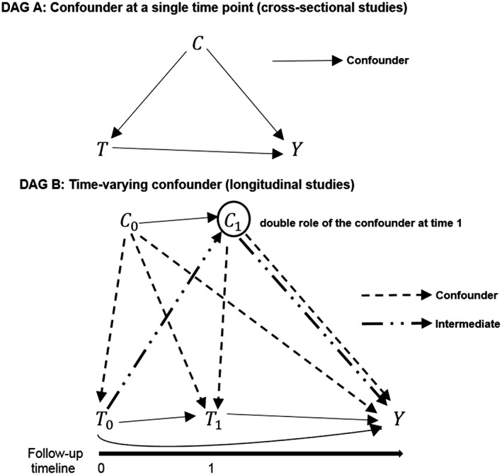
DAG A: Relationship between a confounder variable C, a treatment variable T, and an outcome variable Y in a time point study. DAG B: Relationships between a time‐varying exposure, a time‐varying confounder (which also acts as an intermediate factor), and an outcome variable in a longitudinal study. The double role of the confounder level C₁ is indicated drawing a double arrow. The observations at each time point of the time‐varying exposure and the time‐varying confounder are indicated, respectively, with T₀, T₁, C₀, and C₁ since they are measured at time 0 and at time 1. The variable Y indicates the outcome. For simplicity of the graphical representations, in DAG A and in DAG B a variable representing the set of potential unmeasured confounders has been omitted

4.1. Methods without any adjustment strategy

In many studies, methods that do not take into account time‐varying confounding factors have been used, attempting to estimate the association between the treatment and the outcome conditioning only on the baseline characteristics of the subjects (ITT approach). These kinds of methods essentially assume that the randomization balance of the treatment is preserved, in the sense that each subject receives the randomly assigned treatment during the entire follow‐up. However, the assumption of treatment randomization, either at baseline or over time, does not hold in pharmacoepidemiological investigations using observational data. Consequently, the ITT approach, which only considers baseline exposure and does not adjust for the time dependency of the confounders is not a proper estimation method for longitudinal studies, because it does not guarantee the comparability over time of the groups of interest.

4.2. Models with time‐varying covariates and propensity score‐based methods

Usually baseline (or time‐fixed) values of potential confounding factors are used to estimate the propensity score. However, a time‐varying propensity score to be added to the outcome model could be estimated to consider the variability of the data. Regression methods with time‐varying covariates21, 22, 23, 24, 25, 26, 27 or time‐varying propensity score can be used to adjust for time‐varying confounders only in the scenario that the time‐varying confounders are not affected by previous levels of the exposure, ie, they are not intermediates between the exposure and the outcome. In the most common scenario where the time‐varying confounder is also an intermediate between exposure and outcome, both regression with time‐varying covariates or time‐varying propensity score methods provide biased estimates.28 This adjustment will underestimate or overestimate the total effect of the exposure on the outcome because conditioning on intermediate variables removes from the estimation the indirect effect that the exposure has on the outcome passing through the intermediate variable.28 Using the propensity score for matching or stratification can lead to some bias even if the assumption of no unmeasured confounding holds because the method can fail to completely control for the time dependency of the confounding factors present in the study28 as depicted in Figure 2. Moreover, using time‐varying covariates and or time‐varying propensity score methods to adjust for a time‐varying confounder that is also intermediate may cause bias because such methods do not take into account the possibility that unmeasured confounders between intermediate factors and outcome can exist.29

Figure 2.

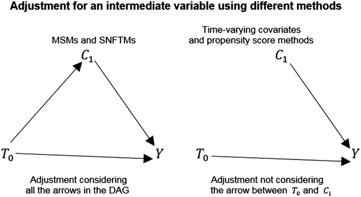
Two DAGs representing how different statistical methods account for a variable that acts as intermediate. MSMs and SNFTMs consider all the arrows that connect the level of the variable C with the level of the treatment variable T and an outcome variable Y. Methods such as regression models with time‐varying covariates and propensity score methods cannot adjust in the analysis for the arrow going from the value of the treatment variable T₀ and the value of the confounder variable C₁so removing from the estimation the indirect effect that the exposure to the treatment has on the outcome passing through the intermediate variable. For simplicity of the graphical representation, in the DAGs, a variable representing the set of potential unmeasured confounders has been omitted

4.3. Marginal structural models

Marginal structural models (MSMs)30, 31, 32 are mainly, but not exclusively, observational‐based methods and an important statistical tool proposed by Robins to adjust for time‐varying confounders. These models work under an extension for longitudinal data, of the potential outcomes framework proposed by Rubin.33 One of the most common and intuitive ways to estimate the parameters of a MSM is using the inverse probability of treatment weighted estimator (IPTW). The IPTW method enables accounting for both baseline and time‐varying confounders. A weighting system gives each unit under observation a weight corresponding to an inverse function of the probability to be exposed conditional on the history of the previous level of the exposure and baseline and time‐varying confounders. In the stabilised weights, the numerator is given by the probability of being exposed conditional on the history of the previous level of the exposure and only baseline confounders. To reduce the variability deriving by dominant subjects in the study, stabilised weights are recommended rather than the “non‐stabilised” weights (with numerator equal to one34), especially in the presence of strong correlation among the covariates and the treatment. The weight at each time point for each unit under observation incorporates the past weights' history multiplicatively. When the underlying assumptions of stable unit treatment value, correct model specification of the weights model, sequential positivity, and no unmeasured confounders35 hold, the IPTW creates a pseudo‐population in which the assignment of the treatment is like randomised, because controlling for the time‐varying confounders ensures both that they no longer are affected by the previous treatment levels and that they do not affect the subsequent treatment levels. A MSM is particularly useful in the case the time‐varying confounder is also an intermediate between the treatment and the response because it produces unbiased estimates of the effect of interest not conditioning on the intermediate variable.28 The main appeal of MSMs is the fact that they are a natural extension of the classical logistic and Cox model, i.e., a marginal structural logistic model is a weighted logistic model where the weights are constructed following the above technique, and similarly a marginal structural Cox model25 can be implemented. Some particular scenarios, as for example strong association between covariates and exposure, and deviation from one of the weight expectation, make it difficult to draw robust inferences from the MSM parameter estimates.36 One main limitation in the application of MSMs, as well as all the more advanced methods, is the lack of user‐friendly statistical packages for the most commonly used software where the methods can be fully implemented. Hernán et al. implemented a MSM to estimate the causal effect of zidovudine on the survival of HIV‐positive men.37 The weights for a MSM can be implemented in the R package ipw 38 which offers the possibility to estimate the weights but not the final MSM. In the website of the Harvard School of Public Health (https://www.hsph.harvard.edu/causal/software/), an example of the code to implement a marginal structural Cox model is provided in Stata and SAS.

4.4. Structural nested failure time models

In the context of survival analysis, SNFTMs are observational‐based methods that allow the unbiased estimation of the causal effect of an exposure on a time to event outcome, in the presence of time‐varying confounders that are also intermediates. An important assumption behind the model is the presence of the counterfactual failure times—time of death or time of another event of interest, e.g., time of the onset of a disease39—for each unit under study. Each individual must be a potential receiver of all possible treatment histories in such a way to have a counterfactual failure time under each possible treatment path. The counterfactual (counter to the facts) yields intuitive understanding that those failure times are potential outcomes for each individual, but that they could not actually have occurred, because each individual can only have 1 factual treatment history. A causal association between an exposure and an event of interest can be derived contrasting counterfactual failure times representing different treatment regimes. Suppose that the parameter of interest of a pharmacoepidemiological study is the average treatment effect40 of a certain drug in the survival of the study population. It can be defined as the difference in survival among treated and untreated individuals. Therefore, the average treatment effect can be derived through a SNFTM contrasting the average counterfactual event times under treatment with the average counterfactual event times under no treatment. The model for the estimation of the counterfactual failure times relates them to both observed treatment history and failure time, so that they can be estimated only for individuals with an observed failure time. The parameter of a SNFTM can be estimated with the g‐estimation procedure.41 The g‐estimation procedure has been less popular in applications, probably due to the computational intensity and the low intuitiveness with respect to the more applied MSMs.42 An advantage of SNFTMs over MSMs is that interactions among covariates and treatment variable can be considered in the model. SNFTMs provide valid statistical inferences of a drug effect of interest under stable unit treatment value and no unmeasured confounding. Chevrier et al.43 implemented a SNFTM with g‐estimation procedure to estimate the effect of exposure to metalworking fluids, when a healthy‐worker survivor effect is present, performing a comparison with other standard methods. To the best of our knowledge, the only available code that can be used as a reference for implementing a SNFTM is available at the website of the Harvard School of Public Health (https://www.hsph.harvard.edu/causal/software/).

5. METHODS FOR CUMULATIVE EXPOSURE AND LATENCY

In designing studies to investigate effects of a particular treatment, researchers should consider that different outcomes can occur at different instances and have different latency periods3 (time to initiation of the treatment to diagnosis). Therefore, different drugs require different exposure periods in relation to the latency. However, these latent periods are usually unknown, and a long follow‐up period allows different assumptions about latent periods to be tested. Different side effects, for example allergic reactions, infections, cardiovascular consequences, or cancers, require different times since exposure to occur. Moreover, while for some outcomes being exposed once is sufficient to consider the subject as exposed, the exposure to high cumulative duration or high cumulative dose is crucial for the majority of the associations. Consequently, the exposure definition and the temporal window considered should be a function of the particular outcome of interest in the plan of a study. For example, a short follow‐up would be sufficient, and simple estimation methods can be appropriate to investigate the association between a certain type of drug and allergic reactions or infections. However, a longer follow‐up and consequently more advanced methods are needed in investigating the association between a drug and a long‐term outcome, such as cancer. Several methods have been introduced which attempt to model a cumulative exposure and the latency, from less flexible approaches where the latency needs to be specified by a prior parametric function,44 to more flexible approaches where the latency is modelled with flexible cubic splines techniques.45, 46 In the next section, some of these methods are discussed.

5.1. Methods without any adjustment strategy

Considering the problem of interest related to outcomes that occur in long term after the exposure, the use of models that do not take into account in any way the time since exposure and the magnitude of the exposure will produce biased results. Moreover, the outcome of interest should be properly considered in the study design. In this sense, when data are available, the duration of the follow‐up should be appropriate for the outcome. The use of the same temporal window, for example, to investigate the effect of a particular treatment on the onset of allergic reactions and cancers will not be a good practice, because this approach will assume that time since exposure, duration of exposure, and cumulative dose have the same effect on both outcomes. A non‐acute adverse outcome such as cancer can be developed many years after the beginning of the exposure, requiring longer follow‐up and quantification of the exposure, whereas an acute allergic reaction can occur shortly after the first dose, requiring shorter follow‐up and a simpler exposure definition.

5.2. Weighted cumulative dose (WCD) model

Dixon et al. reported that the effect of glucocorticoid therapy on the risk of serious infection can change on the basis of how the exposure was modelled. They compared several different standard modelling approaches with a flexible WCD model47 introduced by Sylvestre et al. in 2009. A flexible WCD model attempts to consider 2 important factors in a time‐varying analysis: firstly, that the effects of the exposure can cumulate over time, and secondly, that the different time points of the exposure have different impacts on the outcome. In the study performed by Dixon et al., the exposure was modelled as a weighted sum of doses, with the weighting system reflecting the importance of the different time points of consumption of the dose. The functional form of the weights can be estimated using cubic regression B‐spline. In the approach proposed by Sylvestre, the functional form of the weights is estimated from the data using a regression spline‐based method for modelling the time‐varying cumulative exposure. The final model for the survival analysis is a Cox model with a time‐varying covariate representing the cumulative weighted exposure. The semi‐parametric estimation of the weighted cumulative exposure function does not require the researcher to specify a prior functional form for a continuous exposure avoiding misspecification problems. A potential limitation of the method is that in this time‐varying data structure, time‐varying confounders that act as intermediates are not accounted for, because a Cox model with time‐varying covariates cannot properly adjust for them. A WCD can be implemented with the R package WCE developed by Sylvestre et al. and available in the Comprehensive R Archive Network (CRAN) website (http://cran.r‐project.org/web/packages/WCE).

5.3. Fractional polynomials for the effect of cumulative duration of exposure

Fractional polynomials is a method introduced by Royston et al. in 199448 to model the functional form of the relationship between a continuous independent variable and a dependent variable. This approach has been readapted to model the association between a cumulative duration of exposure to a treatment and an outcome of interest, especially adverse outcomes. The cumulative duration of exposure can be incorporated in the final regression model selecting a proper fractional polynomial transformation. The main advantage of the method is the possibility to model time‐varying covariates effects, allowing for the variation over each time point of the follow‐up, of the effects of such covariates on the outcome. It also allows to avoid assumptions on the functional form of the hazard. In studies of the potential adverse outcomes of a treatment, the duration and dosage of the received treatment play an important role in the analysis. As in the WCD model approach, the final model for the survival analysis is a Cox model with a time‐varying covariate representing the cumulative duration of exposure. Austin et al. in 2014 applied the methods in 2 case studies, one on the association between the cumulative duration of previous amiodarone use and thyroid consequences, and the other investigating association between bisphosphonates use and atypical femoral fractures in women older than 68 years of age. They demonstrated the role of this method in modelling cumulative exposure‐adverse outcomes relationships, providing also guidelines for the use of this method to more general problems. Also, in this case, a potential limitation of the method is that time‐varying confounders acting as intermediates are not accounted for. Fractional polynomials can be implemented using the R package mfp available in the CRAN website (https://cran.r‐project.org/web/packages/mfp/).

6. METHODS FOR TREATMENT SWITCHING

In longitudinal studies assessing a treatment effect, the fact that patients can switch treatment during the follow‐up is a common issue. The reasons for switching can be different, ranging from adverse reactions, failure of therapeutic effects, to the individual behaviour of the patient in the compliance to the treatment.49 The DAG for the time‐varying confounder problem of Figure 1 can be extended to the switching problem as shown in Figure 3. The switching process from a treatment to an alternative treatment can be represented in a DAG (Figure 3) with a time‐varying indicator variable (S₁) describing if the patient remains under the initial treatment or passes to an alternative. The potential relationships between the switching indicator variable S₁ and the other variables under study are depicted with bolded arrows in the DAG. The graph shows that the switching process cannot be considered at random because it may be affected by many variables under study, and it may also affect the outcome of interest. To avoid bias in the investigation of drug effects, researchers should account for the mechanism behind the switching and not consider it a random process. Many methods have been proposed and used in studies affected by switching, but not all of them properly adjust for the confounding arising.4, 50

Figure 3.

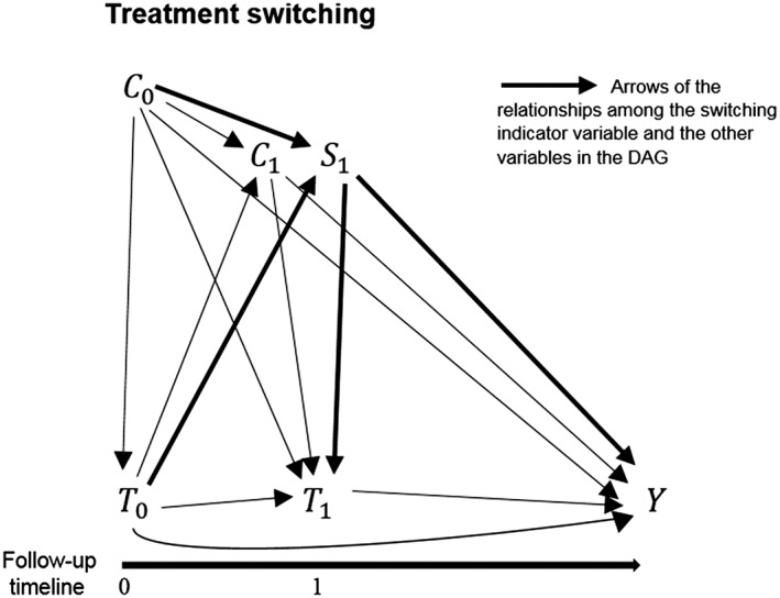
DAG depicting the potential relationships between a time‐varying exposures T, a time‐varying confounder C (which is also intermediate), a switching variable S, and an outcome variable Y in a longitudinal study. The observations at each time point of the time‐varying exposure and the time‐varying confounder are indicated, respectively, with T₀, T₁, C₀, and C₁since they are measured at time 0 and at time 1. The observation of the switching variable is indicated with S₁, measured at time 1 when patients may start to switch to an alternative treatment. The variable Y indicates the outcome. For simplicity of the graphical representation, in the DAG has been omitted a variable representing the set of potential unmeasured confounders

6.1. Methods without any adjustment strategy

Unadjusted regression methods are also used in the presence of treatment switching. The assumption behind such methods is that the treatment switching is a random mechanism and can be ignored in the estimation of a treatment effect because it does not affect the outcome of interest. Such methods adjust only for baseline confounders and evaluate the treatment effect as if all individuals remain under the assigned treatment until the end of the follow‐up (ITT approach).

6.2. Excluding and censoring switchers

Another category of methods evaluates the treatment effect excluding or censoring switchers from the analysis. Like methods without any adjustment strategy, the main assumption behind these approaches is that the switching happens at random such that it can be ignored in the investigation. Excluding and censoring switchers assume that there are no confounders that affect both the switch and the outcome, and moreover censoring switchers is equivalent to assuming that the censoring is not informative, in such a way that it is not related to the outcome.4 This is not a valid assumption and it may cause bias.

6.3. Models with time‐varying covariates

In some applications, the switch is added to a regression model as a time‐varying covariate. A regression model with time‐varying covariates produces unbiased estimates only in the case of no time‐varying confounders2, 37 that are also affected by the previous treatment levels. Moreover, adding a time‐varying covariate for the switch assumes that the switch is not an intermediate variable, and in this sense it is not affected by the prior treatment levels while affecting the outcome. This assumption is unlikely to hold because the prior treatment level is often one of the reasons for switching.

6.4. Marginal structural models with inverse probability of censoring weights

Inverse probability of censoring weighting (IPCW) is a method close to the IPTW estimator. Because in practice, longitudinal studies are often affected by both time‐varying confounders and switching, a MSM incorporating weights for both confounders and switching can be a useful tool. The weights for the non‐switchers are constructed to create a pseudo‐population in which all individuals have the counterfactual outcome as if they have never switched treatment. The model for the weights is based on an inverse function of the probability of not switching conditional on the history of the previous level of the exposure and baseline and time‐varying confounders. To recreate the population that would have been, in the case no switching had occurred, switchers are censored from the analysis, but they are represented through larger weights given to non‐switchers with similar history as the switchers. The advantages and limitations of MSM with IPCW are the same as reported in the time‐varying confounders section. However, another factor should be considered in the switching scenario. In the case the switching depends on clinical reasons (as for example tolerance to the treatment), the switcher should not be censored, but left in the analysis. Diaz et al. used a MSM with IPCW to perform an indirect comparison between the drugs pazopanib and sunitinib used in advanced renal cell carcinoma51 comparing MSM with IPCW to both simpler and other advanced methods. For the implementation of a MSM with IPCW, the R package ipw is available in the CRAN website (https://cran.r‐ project.org/web/packages/ipw/) for the estimation of the weights, and the code provided in the website of the Harvard School of Public Health (https://www.hsph.harvard.edu/causal/software/) can be used as reference to fully implement a MSM with IPCW.

6.5. Structural nested failure time models

SNFTMs produce an unbiased estimate of the effect of a treatment on a survival outcome also in the presence of treatment switching. In the time‐varying confounders scenario, the method is used to estimate the counterfactual times to event of all the individuals with an observed failure time. In the switching context, the method can be used to estimate the counterfactual event times for patients who switch treatment as if they would not have switched. In this situation, to estimate the counterfactual times for the switchers, their observed times to event become the sum of the time during which the patients were under treatment and the time that the patients were not under treatment. In such a way, the overall survival can be derived accounting also for the counterfactual event times of the switchers. The method estimates the overall survival relative to a specific treatment, constructing a pseudo‐population that hypothesises what would have happened to the survival of the switchers, if they would not have switched to the alternative treatment. The pseudo‐population derived through this method attempts to emulate the original randomization of the treatment. The complexity of the method increases with more treatment choices under comparison and with the number of switchers, because the counterfactual event times should be calculated for all the switchers for each treatment line. The advantages and limitations of the method are the same as reported in the time‐varying confounders section. Korhonen et al.5 used a rank‐preserving structural failure time (RPSFT) model (a subcase of SNFTMs for clinical trials) in the RECORD‐1 trial of effectiveness of Everolimus in metastatic renal‐cell carcinoma. To the best of our knowledge, the same as for the time‐varying confounders problem, the only available code that can be used as reference to implement a SNFTM is provided in the website of the Harvard School of Public Health (https://www.hsph.harvard.edu/causal/software/).

7. DISCUSSION

This paper is an attempt to address methodological issues related to time‐varying data in pharmacoepidemiological studies by a critical, and not general, review of the literature. We focused our exposition on four problems related to longitudinal data: construction of treatment episodes, time‐varying confounders, cumulative exposure and latency, and treatment switching. For each of the topics, several methodologies have been identified and described. The characterisation of the methods is not intended to provide an analytical illustration, but rather a conceptualization of the theoretical approach adopted attempting to address the involved complications.

In constructing treatment episodes, researchers used a number of approaches including methods using DDD assumption, methods accounting for overlap and gaps between drug prescriptions, and methods prospectively filling gaps to avoid bias.

When data on exact dose are missing, the use of the DDD assumption may be a useful standard to provide comparability of the studies. On the other hand, 1 DDD per day may not be the dose actually prescribed or consumed by the individual patient and may result in misclassification bias. Methods accounting for overlap and gaps between drug prescriptions and methods prospectively filling gaps are useful tools to properly build treatment episodes accounting for gaps and overlaps existing in prescription registers.

The choice of method to construct treatment episode depends on the therapeutic area of interest. In some therapeutic areas for example the assumption of consumption of 1 DDD per day of the prescribed drug may hold because it is close to the real dosage prescribed by the physicians. In other therapeutic areas, the real prescribed dosage may be very different. In the definition of the allowed gap, the particular type of treatment plays an important role; in fact, treatments can be long or short term, occasional or limited to 1 prescription. Generally, it is a good practice to allow gaps of few days for short term treatments and longer gaps for long‐term treatments.1 It is also recommended to perform a sensitivity analysis to assess how different assumptions influence the effect estimates.

A time‐varying exposure can be followed by the presence of time‐varying confounders, and different methods have been used including methods without any adjustment strategy, models with time‐varying covariates, and propensity score‐based methods, MSMs, and SNFTMs. Methods without any adjustment strategy, models with time‐varying covariates, and propensity score methods provide biased results in the presence of time‐varying confounders that act as intermediates between the exposure and the outcome. Conversely, MSMs and SFTMs can provide unbiased estimates of the treatment effect under the main assumption of no unmeasured confounders. The need of more user‐friendly statistical packages for the most advanced and complex methods calls for further research in this field to make a more extended use of appropriate methods.

For cumulative exposure and latency, the investigated approaches are methods without any adjustment strategy, WCD models, and fractional polynomials for the effect of cumulative duration of exposure. More advanced methods such as WCD models and fractional polynomials, and also longer follow‐up time, are recommended for long‐term outcomes. These advanced methods are useful tools when the effect of a treatment or a covariate on the outcome varies during follow‐up. Such methods account for the fact that the time since exposure has an impact on the response variable. One limitation of the methods is that potential time‐varying confounders that are also intermediates cannot be included as time‐varying covariates in the model because such strategy may provide a biased estimate of the treatment‐response relationship. In the presence of time‐varying confounders, a cumulative exposure could be modelled using a method such as MSM, but the assumption of no unmeasured confounders should be taken into account by the researchers.

For treatment switching, the investigated approaches are as follows: methods without any adjustment strategy, excluding and censoring switchers methods, models with a time‐varying covariate for the switching, MSMs with IPCW, and SNFTMs. Methods without any adjustment strategy, excluding and censoring switchers methods, and models with time‐varying covariates produce biased results because the switching mechanism is not properly accounted for. Conversely, MSMs with IPCW and SFTMs models correctly adjust for the switching mechanism under the main assumption of no unmeasured confounders. As previously stressed, more statistical packages implementing the advanced methods are greatly needed.

In longitudinal studies, a proper exposure definition, considering all the aspects of the magnitude of the exposure, such as duration and quantity, is strongly advised. Moreover, the presence of time‐varying confounders or treatment switching can lead to problems in the correct estimation of the effect of interest. In the literature, many applications do not consider the problem using methods that do not properly adjust for the bias introduced by a confounder that acts also as intermediate or a switching process. Methods such as MSMs and SNFTMs correctly adjust for such confounding, but the assumption of no unmeasured confounders in the use of these methods should be taken into account by the researchers. The applicability of such advanced methods depends strongly on the quality and the completeness of the data.

In the literature, many advanced methods have been proposed to try to address issues connected with longitudinal studies, but the most advanced methods are not commonly implemented. One of the reasons for this underuse of the methods could be the methodological complexity and the limited availability of implementation packages in commonly used statistical software.

Several advanced methods are developed that provide less biased results and hence can help to guide clinical decision making. However, these methods should be implemented and compared in order to identify which provide reasonably accurate results but is not overly complex to use and interpret. Further research on the application and implementation in pharmacoepidemiology of the most advanced and complex methods, as MSMs and SNFTMs, is needed. Construction of treatment episodes and models accounting for cumulative exposure and latency are research areas with a wide perspective for further investigations.

ETHICS STATEMENT

The authors declare that no ethical approval was needed for the study.

CONFLICT OF INTEREST

The Centre for Pharmacoepidemiology receives grants from several entities (pharmaceutical companies, regulatory authorities, and contract research organisations) for performance of drug safety and drug utilisation studies.

Emese Vago, Paul Stang, Mingliang Zhang, and David Myers are employees of Janssen Research and Development. The authors declare no other conflict of interest.

Pazzagli L, Linder M, Zhang M, et al. Methods for time‐varying exposure related problems in pharmacoepidemiology: An overview. Pharmacoepidemiol Drug Saf. 2018;27:148–160. https://doi.org/10.1002/pds.4372

REFERENCES

- 1. Gardarsdottir H, Souverein PC, Egberts TCG, Heerdink ER. Construction of drug treatment episodes from drug‐dispensing histories is influenced by the gap length. J Clin Epidemiol. 2010;63(4):422‐427. https://doi.org/10.1016/j.jclinepi.2009.07.001 [DOI] [PubMed] [Google Scholar]
- 2. Robins JM, Hernan MA, Brumback B. Marginal structural models and causal inference in epidemiology. Epidemiology. 2000;11(5):550‐560. https://doi.org/10.1097/00001648‐200009000‐00011 [DOI] [PubMed] [Google Scholar]
- 3. Dixon WG, Abrahamowicz M, Beauchamp ME, et al. Immediate and delayed impact of oral glucocorticoid therapy on risk of serious infection in patients with rheumatoid arthritis: a nested case‐control analysis using a weighted cumulative dose model. Arthritis Rheum. 2011;63:S960‐S960. [DOI] [PMC free article] [PubMed] [Google Scholar]
- 4. Latimer NR, Abrams KR, Lambert PC, et al. Adjusting for treatment switching in randomised controlled trials—a simulation study and a simplified two‐stage method. Stat Methods Med Res. 2014;26(2):724‐751. https://doi.org/10.1177/0962280214557578 [DOI] [PubMed] [Google Scholar]
- 5. Korhonen P, Zuber E, Branson M, et al. Correcting overall survival for the impact of crossover via a rank‐preserving structural failure time (Rpsft) model in the Record‐1 trial of everolimus in metastatic renal‐cell carcinoma. J Biopharm Stat. 2012;22(6):1258‐1271. https://doi.org/10.1080/10543406.2011.592233 [DOI] [PubMed] [Google Scholar]
- 6. Young JG, Hernan MA, Picciotto S, Robins JM. Relation between three classes of structural models for the effect of a time‐varying exposure on survival. Lifetime Data Anal. 2010;16(1):71‐84. https://doi.org/10.1007/s10985‐009‐9135‐3 [DOI] [PMC free article] [PubMed] [Google Scholar]
- 7. Rosholm JU, Andersen M, Gram LF. Are there differences in the use of selective serotonin reuptake inhibitors and tricyclic antidepressants? A prescription database study. Eur J Clin Pharmacol. 2001;56(12):923‐929. https://doi.org/10.1007/s002280000234 [DOI] [PubMed] [Google Scholar]
- 8. Merlo J, Wessling A, Melander A. Comparison of dose standard units for drug utilisation studies. Eur J Clin Pharmacol. 1996;50(1‐2):27‐30. https://doi.org/10.1007/s002280050064 [DOI] [PubMed] [Google Scholar]
- 9. Romppainen T, Rikala M, Aarnio E, Korhonen MJ, Saastamoinen LK, & Huupponen R. Measurement of statin exposure in the absence of information on prescribed doses. Eur J Clin Pharmacol. 2014;70(10):1275‐1276. https://doi.org/10.1007/s00228‐014‐1737‐3 [DOI] [PubMed] [Google Scholar]
- 10. Sihvo S, Wahlbeck K, McCallum A, et al. Increase in the duration of antidepressant treatment from 1994 to 2003: a nationwide population‐based study from Finland. Pharmacoepidemiol Drug Saf. 2010;19(11):1186‐1193. https://doi.org/10.1002/pds.2017 [DOI] [PubMed] [Google Scholar]
- 11. Bjerrum L, Rosholm JU, Hallas J, Kragstrup J. Methods for estimating the occurrence of polypharmacy by means of a prescription database. Eur J Clin Pharmacol. 1997;53:7‐11. https://doi.org/10.1007/s002280050329 [DOI] [PubMed] [Google Scholar]
- 12. Lunde P. In: Bergamn U, ed. Studies in Drug Utilisation. Methods and Applications. Copenhagen: WHO regional Office for Europe; 1979:17‐28. [Google Scholar]
- 13. Gardarsdottir H, Egberts TC, Stolker JJ, Heerdink ER. Duration of antidepressant drug treatment and its influence on risk of relapse/recurrence: immortal and neglected time bias. Am J Epidemiol. 2009;170(3):280‐285. https://doi.org/10.1093/aje/kwp142 [DOI] [PubMed] [Google Scholar]
- 14. Gardarsdottir H, van Geffen ECG, Stolker JJ, Egberts TCG, Heerdink ER. Does the length of the first antidepressant treatment episode influence risk and time to a second episode? J Clin Psychopharmacol. 2009;29(1):69‐72. https://doi.org/10.1097/JCP.0b013e31819302b1 [DOI] [PubMed] [Google Scholar]
- 15. Gichangi A, Andersen M, Kragstrup J, Vach W. Analysing duration of episodes of pharmacological care: an example of antidepressant use in Danish general practice. Pharmacoepidemiol Drug Saf. 2006;15(3):167‐177. https://doi.org/10.1002/pds.1160 [DOI] [PubMed] [Google Scholar]
- 16. Gardarsdottir H, Egberts TCG, Heerdink ER. The association between patient‐reported drug taking and gaps and overlaps in antidepressant drug dispensing. Ann Pharmacother. 2010;44(11):1755‐1761. https://doi.org/10.1345/aph.1P162 [DOI] [PubMed] [Google Scholar]
- 17. Nielsen LH, Lokkegaard E, Andreasen AH, Keiding N. Using prescription registries to define continuous drug use: how to fill gaps between prescriptions. Pharmacoepidem Dr S. 2008;17(4):384‐388. https://doi.org/10.1002/pds.1549 [DOI] [PubMed] [Google Scholar]
- 18. Suissa S. Immortal time bias in pharmacoepidemiology. Am J Epidemiol. 2008;167(4):492‐499. https://doi.org/10.1093/aje/kwm324 [DOI] [PubMed] [Google Scholar]
- 19. van Walraven C, Davis D, Forster AJ, Wells GA. Time‐dependent bias was common in survival analyses published in leading clinical journals. J Clin Epidemiol. 2004;57(7):672‐682. https://doi.org/10.1016/j.jclinepi.2003.12.008 [DOI] [PubMed] [Google Scholar]
- 20. Daniel RM, Cousens SN, De Stavola BL, Kenward MG, Sterne JAC. Methods for dealing with time‐dependent confounding. Stat Med. 2013;32(9):1584‐1618. https://doi.org/10.1002/sim.5686 [DOI] [PubMed] [Google Scholar]
- 21. Laurin LP, Gasim AM, Poulton CJ, et al. Treatment with glucocorticoids or calcineurin inhibitors in primary FSGS. Clin J Am Soc Nephrol. 2016;11(3):386‐394. https://doi.org/10.2215/CJN.07110615 [DOI] [PMC free article] [PubMed] [Google Scholar]
- 22. Wells PS, Gebel M, Prins MH, Davidson BL, Lensing AW. Influence of statin use on the incidence of recurrent venous thromboembolism and major bleeding in patients receiving rivaroxaban or standard anticoagulant therapy. Thromb J. 2014;12:1. [DOI] [PMC free article] [PubMed] [Google Scholar]
- 23. Tzeng H‐E, Muo CH, Chen HT, Hwang WL, Hsu HC, & Tsai CH. Tamoxifen use reduces the risk of osteoporotic fractures in women with breast cancer in Asia: a nationwide population‐based cohort study. BMC Musculoskelet Disord. 2015;16:1. [DOI] [PMC free article] [PubMed] [Google Scholar]
- 24. Sharma TS, Wasko MC, Tang X, et al. Hydroxychloroquine use is associated with decreased incident cardiovascular events in rheumatoid arthritis patients. J Am Heart Assoc. 2016;5(1):e002867. [DOI] [PMC free article] [PubMed] [Google Scholar]
- 25. Shirani A, Zhao Y, Karim ME, et al. Association between use of interferon beta and progression of disability in patients with relapsing‐remitting multiple sclerosis. JAMA. 2012;308(3):247‐256. [DOI] [PubMed] [Google Scholar]
- 26. Moura CS, Abrahamowicz M, Beauchamp ME, et al. Early medication use in new‐onset rheumatoid arthritis may delay joint replacement: results of a large population‐based study. Arthritis Res Ther. 2015;17:1. [DOI] [PMC free article] [PubMed] [Google Scholar]
- 27. Flynn RW, MacDonald TM, Hapca A, MacKenzie IS, Schembri S. Quantifying the real life risk profile of inhaled corticosteroids in COPD by record linkage analysis. Respir Res. 2014;15(1):141. [DOI] [PMC free article] [PubMed] [Google Scholar]
- 28. Ali MS, Groenwold RH, Belitser SV, et al. Methodological comparison of marginal structural model, time‐varying Cox regression, and propensity score methods: the example of antidepressant use and the risk of hip fracture. Pharmacoepidemiol Drug Saf. 2016;25:114‐121. https://doi.org/10.1002/pds.3864 [DOI] [PubMed] [Google Scholar]
- 29. Cole SR, Hernan MA. Fallibility in estimating direct effects. Int J Epidemiol. 2002;31(1):163‐165. https://doi.org/10.1093/ije/31.1.163 [DOI] [PubMed] [Google Scholar]
- 30. Gsponer T, Petersen M, Egger M, et al. The causal effect of switching to second‐line ART in programmes without access to routine viral load monitoring. AIDS. 2012;26(1):57‐65. https://doi.org/10.1097/QAD.0b013e32834e1b5f [DOI] [PMC free article] [PubMed] [Google Scholar]
- 31. Petersen M, Schwab J, Gruber S, Blaser N, Schomaker M, & van der Laan M. Targeted maximum likelihood estimation for dynamic and static longitudinal marginal structural working models. J causal inference. 2014;2(2):147‐185. [DOI] [PMC free article] [PubMed] [Google Scholar]
- 32. Schnitzer ME, Moodie EE, van der Laan MJ, Platt RW, Klein MB. Modeling the impact of hepatitis C viral clearance on end‐stage liver disease in an HIV co‐infected cohort with targeted maximum likelihood estimation. Biometrics. 2014;70(1):144‐152. [DOI] [PMC free article] [PubMed] [Google Scholar]
- 33. Rubin DB. Estimating causal effects of treatments in randomized and nonrandomized studies. J Educ Psychol. 1974;66(5):688‐701. https://doi.org/10.1037/h0037350 [Google Scholar]
- 34. Robins JM. Statistical Models in Epidemiology, the Environment, and Clinical Trials. Springer; 2000:95‐133. [Google Scholar]
- 35. Zhang J, Chen C. Correcting treatment effect for treatment switching in randomized oncology trials with a modified iterative parametric estimation method. Stat Med. 2016;35(21):3690‐3703. https://doi.org/10.1002/sim.6923 [DOI] [PubMed] [Google Scholar]
- 36. Karim ME, Gustafson P, Petkau J, et al. Marginal structural Cox models for estimating the association between beta‐interferon exposure and disease progression in a multiple sclerosis cohort. Am J Epidemiol. 2014;180(2):160‐171. https://doi.org/10.1093/aje/kwu125 [DOI] [PMC free article] [PubMed] [Google Scholar]
- 37. Hernan MA, Brumback B, Robins JM. Marginal structural models to estimate the causal effect of zidovudine on the survival of HIV‐positive men. Epidemiology. 2000;11(5):561‐570. [DOI] [PubMed] [Google Scholar]
- 38. van der Wal WM, Geskus RB. ipw: an R package for inverse probability weighting. J Stat Softw. 2011;43:1‐23. [Google Scholar]
- 39. Yamaguchi T, Ohashi Y. Adjusting for differential proportions of second‐line treatment in cancer clinical trials. Part I: structural nested models and marginal structural models to test and estimate treatment arm effects. Stat Med. 2004;23(13):1991‐2003. https://doi.org/10.1002/sim.1816 [DOI] [PubMed] [Google Scholar]
- 40. Imbens GW, Wooldridge JM. Recent developments in the econometrics of program evaluation. J Econ Lit. 2009;47(1):5‐86. [Google Scholar]
- 41. Robins JM. Structural nested failure time models. Encycl Biostatistics. 1998. [Google Scholar]
- 42. Joffe MM. Structural nested models, G‐estimation, and the healthy worker effect the promise (mostly unrealized) and the pitfalls. Epidemiology. 2012;23(2):220‐222. https://doi.org/10.1097/EDE.0b013e318245f798 [DOI] [PubMed] [Google Scholar]
- 43. Chevrier J, Picciotto S, Eisen EA. A comparison of standard methods with G‐estimation of accelerated failure‐time models to address the healthy‐worker survivor effect application in a cohort of autoworkers exposed to metalworking fluids. Epidemiology. 2012;23(2):212‐219. https://doi.org/10.1097/EDE.0b013e318245fc06 [DOI] [PubMed] [Google Scholar]
- 44. Richardson D, Latency B. Models for analyses of protracted exposures. Epidemiology. 2009;20(3):395‐399. https://doi.org/10.1097/EDE.0b013e318194646d [DOI] [PMC free article] [PubMed] [Google Scholar]
- 45. Abrahamowicz M, MacKenzie TA. Joint estimation of time‐dependent and non‐linear effects of continuous covariates on survival. Stat Med. 2007;26(2):392‐408. https://doi.org/10.1002/sim.2519 [DOI] [PubMed] [Google Scholar]
- 46. Berhane K, Hauptmann M, Langholz B. Using tensor product splines in modeling exposure‐time‐response relationships: application to the Colorado plateau uranium miners cohort. Stat Med. 2008;27(26):5484‐5496. https://doi.org/10.1002/sim.3354 [DOI] [PMC free article] [PubMed] [Google Scholar]
- 47. Sylvestre MP, Abrahamowicz M. Flexible modeling of the cumulative effects of time‐dependent exposures on the hazard. Stat Med. 2009;28(27):3437‐3453. https://doi.org/10.1002/sim.3701 [DOI] [PubMed] [Google Scholar]
- 48. Royston P, Altman DG. Regression using fractional polynomials of continuous covariates: parsimonious parametric modelling. Appl stat. 1994;43(3):429‐467. [Google Scholar]
- 49. Watkins C, Huang X, Latimer N, Tang YY, Wright EJ. Adjusting overall survival for treatment switches: commonly used methods and practical application. Pharm Stat. 2013;12(6):348‐357. https://doi.org/10.1002/pst.1602 [DOI] [PubMed] [Google Scholar]
- 50. Latimer NR, Abrams KR, Lambert PC, et al. Adjusting survival time estimates to account for treatment switching in randomized controlled trials‐an economic evaluation context: methods, limitations, and recommendations. Med Decis Making. 2014;34(3):387‐402. https://doi.org/10.1177/0272989x13520192 [DOI] [PubMed] [Google Scholar]
- 51. Diaz J, Sternberg CN, Mehmud F, et al. Overall survival endpoint in oncology clinical trials: addressing the effect of crossover—the case of Pazopanib in advanced renal cell carcinoma. Oncology. 2016;90(3):119‐126. https://doi.org/10.1159/000443647 [DOI] [PubMed] [Google Scholar]