Dual‐Sensitivity Multiple Sclerosis Lesion and CSF Segmentation for Multichannel 3T Brain MRI

ABSTRACT

BACKGROUND AND PURPOSE

A pipeline for fully automated segmentation of 3T brain MRI scans in multiple sclerosis (MS) is presented. This 3T morphometry (3TM) pipeline provides indicators of MS disease progression from multichannel datasets with high‐resolution 3‐dimensional T1‐weighted, T2‐weighted, and fluid‐attenuated inversion‐recovery (FLAIR) contrast. 3TM segments white (WM) and gray matter (GM) and cerebrospinal fluid (CSF) to assess atrophy and provides WM lesion (WML) volume.

METHODS

To address nonuniform distribution of noise/contrast (eg, posterior fossa in 3D‐FLAIR) of 3T magnetic resonance imaging, the method employs dual sensitivity (different sensitivities for lesion detection in predefined regions). We tested this approach by assigning different sensitivities to supratentorial and infratentorial regions, and validated the segmentation for accuracy against manual delineation, and for precision in scan‐rescans.

RESULTS

Intraclass correlation coefficients of .95, .91, and .86 were observed for WML and CSF segmentation accuracy and brain parenchymal fraction (BPF). Dual sensitivity significantly reduced infratentorial false‐positive WMLs, affording increases in global sensitivity without decreasing specificity. Scan‐rescan yielded coefficients of variation (COVs) of 8% and .4% for WMLs and BPF and COVs of .8%, 1%, and 2% for GM, WM, and CSF volumes. WML volume difference/precision was .49 ± .72 mL over a range of 0–24 mL. Correlation between BPF and age was r = .62 (P = .0004), and effect size for detecting brain atrophy was Cohen's d = 1.26 (standardized mean difference vs. healthy controls).

CONCLUSIONS

This pipeline produces probability maps for brain lesions and tissue classes, facilitating expert review/correction and may provide high throughput, efficient characterization of MS in large datasets.

Introduction

Multiple sclerosis (MS) is a chronic inflammatory and degenerative disease of the CNS, and a major contributor to physical disability and cognitive dysfunction.1, 2 Although gray matter (GM) degeneration is also observed, MS mainly affects the white matter (WM), with multiple demyelinating lesions that are the name‐giving hallmark of MS. Together with parenchymal atrophy, magnetic resonance imaging (MRI)‐based detection and tracking of MS lesions yields established diagnostic and therapeutic outcome markers.3, 4, 5

Several algorithms for automated lesion volumetrics have been introduced,6, 7, 8, 9, 10, 11, 12 but most are invariably tailored to specific image characteristics of resolution and contrast and not easily adapted to different acquisition protocols. They also commonly lack interfaces to introduce protocol‐specific regional heuristics. A well‐established principle used in automated WM lesion (WML) segmentation is to define lesions as outliers of the WM intensity distribution,9, 10 rather than seeking to model and segment them directly. This is most commonly implemented via an expectation‐maximization (EM) algorithm,13 or a fuzzy C‐means classifier instead of EM in conjunction with anatomical atlases,8 or the introduction of a trimmed‐likelihood estimator (instead of the maximum‐likelihood commonly implemented in EM) to improve robustness against outliers that otherwise bias the building of intensity distribution models.14 More complex pipelines isolate regions like the cerebellum with typical signal bias into a separate segmentation,7 similar in principle to the dual‐sensitivity approach in the 3T morphometry (3TM) pipeline presented here.

An intuitive two‐phase approach separated the task of WML detection from the task of delineation.6 It also used outliers to WM intensity distribution as initial WML candidates, but obtained the final segmentation through a subsequent region‐growing approach from the initial seed points, which proffers the advantage of considering local contrast (vs. absolute intensity) in the final delineation and thus can produce segmentations that agree well with the visual interpretation of an expert. Trained classifiers can provide excellent accuracy of lesion segmentation,15 but multiple reference segmentations are commonly required for training, which implies that a retraining would be necessary when the underlying image characteristics change. Some level of robustness can be achieved by the addition of spatial priors and intensity normalization,16 but the need for retraining remains, which is costly if a new reference training set has to be obtained. For additional background, we refer the reader to a comprehensive review of WML segmentation methods.17

The 3TM strategy does not represent a new segmentation algorithm per se, but a comprehensive processing pipeline to extend the applicability of such standalone algorithms with a larger constraint framework to facilitate routine application of MR morphometry, similar in concept to the size and intensity constraints described previously.18 Our main objectives in the present study were to: (1) incorporate an additional level of abstraction as a mechanism to translate anatomical heuristics into standard (Euclidian) spatial priors; (2) facilitate adjustments and recalibration to address changes in image acquisition parameters, scanner hardware, or software changes or scanner drift; and (3) provide an intuitive framework to address the spatial variation of image characteristics (eg, SNR or contrast) that become increasingly relevant at higher field strengths.

Given the wide and skewed distribution of lesion burden in longstanding MS, most clinical uses of MR volumetry, both longitudinal and cross sectional, tend to benefit more from robustness and precision than accuracy, ie, some level of systematic bias is preferable to the reduced sensitivity that is commonly introduced when tuning for optimal accuracy. This effect tends to be exacerbated as the range of disease burden widens. For example, the importance of addressing intensity variations was demonstrated by the significant improvement of k‐Nearest Neighbor (kNN)‐algorithms through different forms of intensity normalizations.16

The 3TM method presented herein defines MS WMLs as outliers in the image signal intensity distribution of WM,10 using an EM algorithm13 and a WM segmentation map as a spatial prior. Unlike the abovementioned methods, no generic probabilistic atlas is used as an anatomical prior. This reflects our current experience that overall accuracy and particularly sensitivity for juxtacortical lesions critically depends on accurate spatial priors. For such areas of high anatomical variance, in our experience, more accurate priors are obtained by direct segmentation than by an intersubject registration, despite the presence of pathology. A configurable set of heuristic rules corrects misclassifications in the anatomical prior (WM, gray matter [GM], cerebrospinal fluid [CSF]; for definitions, see Table 1) that originate from common artifacts or pathology.

Table 1.

Definitions

Term/Metric	Definition/Description
WM	Cortical and subcortical white matter
GM	Cortical and subcortical gray matter
cGM, cerGM	Cortical and cerebellar GM, respectively
CSF	Cerebrospinal fluid, including cortical and ventricular (lateral, third and fourth ventricles), and subarachnoid space overlying the brain surface
vCSF	Ventricular CSF, portion of the CSF class comprising the lateral, third and fourth ventricles
ICV	Intracranial volume, comprising all brain parenchyma including cortical and ventricular CSF, excluding the dura, ending inferiorly at the medulla. Segmented as part of the pipeline preprocessing (see Table 2, step 3)
BPF	Brain parenchymal fraction, defined as 1‐CSF/ICV, ie, brain parenchymal volume, normalized by the total intracranial volume
WML	White matter lesions, defined as regions of abnormally hyperintense (FLAIR, T2), exclusively within the WM
Infratentorial region	Anatomical structures inferior to the cerebellar tentorium, including structures of the cerebellum and brainstem. Defined based on the anatomical parcellation in the 3TM pipeline (see Table 2, step 4)

A “dual sensitivity” concept is introduced in our pipeline, which compiles the final segmentation from multiple runs of the EM algorithm at different sensitivity settings for predefined anatomical regions. The applied dual sensitivity concept departs from the assumption of spatially constant WM or WML properties, but instead builds on the premise that WM tissue properties vary regionally, and that this variation is exacerbated with advanced diffuse disease burden and further modulated by spatially variant noise of MRI scan sequences and the increasing inhomogeneity of higher field magnets. This is of critical relevance to the application of automated morphometry with a wide spectrum of disease burden and a background of sporadically changing MR protocols. The application of MS lesion morphometry in routine clinical care further implies a trade‐off between sensitivity and specificity that varies based on disease severity and duration: sensitivity is paramount in new and low disease burden, where false positives are preferable to false negatives in the assessment and monitoring of disease activity, which is crucial for treatment evaluation. With advanced (high) disease burden, robustness and precision become more important, and the manual correction and detection of change becomes prohibitive in effort.

A key feature of our 3TM method is an easy parameter tuning to optimize between varying and competing demands for sensitivity and specificity, a rationale arising from the objective of applying automated segmentation not only in controlled studies but also in clinical routine. This is realized by its modular design and the consistent exposure of parameters as well as abstraction layers for defining heuristic rule sets. Common reasons for adjustments are: (1) the need for higher sensitivity based on MS disease duration and severity; (2) the relative reliability of the different MRI channels and their specificity for segmentation; (3) the prevalence of false positives due to sequence‐specific artifacts; and (4) the implementation of heuristic rules to automatically recover from common false negatives like the misclassification of subcortical lesions as GM, or false positives from misclassifications of the choroid plexus as WMLs.

Methods

Subjects

Our test cohort included 29 patients with MS (20 women), age 47 ± 10 years (mean ± SD, range 24–70 years), with disease duration 12.5 ± 6.5 years (range 1–27 years) and Expanded Disability Status Scale (EDSS) scores 2.5 ± 1.6 (median ± SD; range 0–6). Disease subtypes were relapsing‐remitting (n = 21), secondary progressive (n = 5), primary progressive (n = 2), and clinically isolated demyelinating syndrome (n = 1). The scan‐rescan experiment included a different set of another 13 patients with MS (50 ± 8 years old, with 18 ± 10 years disease duration) and 15 healthy volunteers (38 ± 10 years old); these images have contributed to separate studies, in which the recruitment and acquisition procedures have been detailed.19, 20 The patients with MS were selected to represent a broad spectrum of disease severity to assess accuracy and precision of WML volume and brain atrophy. All subjects were scanned with written informed consent, which was approved by the local ethics committee of Partners Health Care. This human research was in compliance with the Helsinki Declaration.21

MRI

The brain MRI acquisition protocol (3T Siemens Skyra, 20‐channel head coil) comprised three 3‐dimensional high‐resolution sequences with T1‐, T2‐, and fluid‐attenuated inversion‐recovery (FLAIR)‐weighting, optimized in contrast for depicting WM/GM interfaces, CSF, and WMLs, respectively. All sequences were sagittally acquired, covering the whole head, with 1 mm isotropic voxel size. The additional MRI protocol details were: a T1‐weighted gradient echo (TE/TR = 2.96/2,300 milliseconds, TI = 900 milliseconds, flip angle = 9°), T2 spin echo (TE/TR = 300/2,500 milliseconds, echo train length = 160) and T2‐FLAIR (TE/TR = 389/5,000 milliseconds, TI = 1,800 milliseconds, echo train length = 248).

Segmentation Pipeline: Preprocessing

The main steps of the pipeline are outlined in Table 2. Key steps are spatial coregistration of the three core MR sequences, anatomical parcellation with subsequent heuristic correction of common misclassifications, and an EM algorithm to determine the final WM, GM, CSF, and WML segmentations. WMLs were classified as outliers in the WM intensity distribution, applied with dual sensitivity settings for the supratentorial and infratentorial regions, respectively, meaning that the intensity distributions for normal tissue and the outlier threshold estimates were obtained separately for each region. The pipeline is modular and utilizes a combination of existing and custom methods for each module, as detailed in Table 2. The specific methods for the individual steps are exchangeable.

Table 2.

3TM Pipeline Outline

	Module	Objective	Method	Parameters
1	Bias field correction	Removes intensity variation due to in‐homogeneities of coil sensitivity	N434	Three resolution levels, with fourfold subsampling
2	Coregistration	Spatially aligns all series of the exam (FLAIR, T2) to the reference series (T1); removes low‐level spatial distortions	BRAINS/ITK22	6, 7, 12 affine degrees of freedom + BSpline with 5 × 5 × 5 grid, mutual information similarity criterion
3	ICV/brain mask	Skull stripping and ICV mask generation	BET23	Based on T2, repeat runs with parameter range and final voting
4	Anatomic parcellation	Tissue class segmentation and anatomical parcellation. Serves as a rule base for heuristics of step 6 and also as a basis for spatial prior maps of step 8	Freesurfer27	Full parcellation including cortical tessellation (recon‐all)
5	Intensity normalization	Global matching of intensity distributions to a reference scan set (1 per channel, selected from the study dataset). Enables absolute intensities in heuristics of step 6	Custom35	Computes global shift and scale from weighted WM, GM, and CSF class comparisons
6	Heuristic rules	Correct misclassifications in the anatomical parcellation by comparison with the coregistered FLAIR image	Custom	See Table 3
7	Spatial prior maps	Generate individual tissue probability maps for the spatial distribution of WM, GM, and CSF	Custom	Based on the parcellation in step 4
8	EM	Tissue class (WM, GM, CSF) and WML segmentation	Custom EM, based on prior work10	Mahalanobis distance 2.3 for the supratentorial region and 3.0 for the infratentorial region
9	Postprocessing	Island removal and FP reduction	Custom	Minimal lesion size = 3 mm

Note: Listed in sequence are the image processing steps of the 3T morphometry (3TM) automated MS lesion and tissue class segmentation. Principal outputs are anatomical parcellation‐label maps and probability maps for white matter (WM), gray matter (GM), cerebrospinal fluid (CSF), and white matter lesions (WMLs). ICV = total intracranial volume; BET = Brain Extraction Tool; EM = expectation maximization; FP = false positive; FLAIR = fluid‐attenuated inversion recovery.

The intraexam image registration contains affine and nonrigid transformations22 to harmonize the varying amounts of spatial distortions and protocol‐specific distortion corrections present (eg, common differences in distortion correction between the T1 gradient‐echo and T2 and FLAIR spin‐echo‐based sequences).

The intracranial volume (ICV) mask was obtained using a variation of the Brain Extraction Tool (BET) algorithm.23 The T2 series was used as the input to BET to capture the subarachnoid space along the outer brain contour and avoid clipping of cortical CSF. For better robustness, BET was run on a consecutive range of parameters (fractional threshold and radius), summing the results at each step to form a cumulative probability map. This map was then thresholded at an empirically predefined level (the same for all subjects).

While a lesion‐filling scheme24, 25 is possible and compatible with this pipeline, it was not used, since the anatomical parcellation already segmented T1‐hypointensities, and misclassifications are effectively captured by the heuristic rule set (see step 6 in Table 2 and also Table 3). While lesion‐filling is indicated for gray‐white distinctions, its effect on whole‐brain measurements has shown to be negligible.26

Table 3.

Heuristic Rule Set for Correcting Misclassifications

Rule	Location of FP/FN	Description	Target	Reference	Z	D
1	Choroid plexus FN	Hyperintensities inside the lateral ventricles are likely choroid plexus	vCSF	CSF	3.0	–
2	Periventricular Halo (FN)	Mild hyperintensities at the edges of the lateral ventricles are likely WMLs	vCSF	WM	1.8	1
3	Cortical GM FP	Hyperintense GM >8 mm from the cortical surface is likely a WML	cGM	GM	2.5	>8
4	Cerebral GM FP	Very hyperintense GM is likely a WML irrespective of cortex proximity	GM	GM	4.0	–
5	Cerebellar GM FP	Hyperintense GM in cerebellum is likely a WML	cerGM	GM	3.0
6	Caudate FP	Hyperintense caudate is likely a WML	Caudate	Caudate	3.0

Note: A sequence of customizable rules is applied to correct misclassifications in the T1‐based anatomical parcellation. The reference image for the intensity rules in the presented configuration was the fluid‐attenuated inversion‐recovery image. Target = the label class where misclassifications are suspected; Reference = the label class used to build a reference intensity distribution; Z = Z‐score threshold, eg, for rule 3: any voxel labeled as cortical gray matter (GM) with intensities more than 2.5 standard deviations above the mean GM intensity is relabeled. D = minimum or maximum distance in millimeter away from the boundary of the reference structure; vCSF = ventricular cerebrospinal fluid; cGM = cortical GM; cerGM = cerebellar GM; FP/FN = false positive/negative; WML = white matter lesion.

Atlas‐Based Anatomical Parcellation and Heuristic Rule Set

The 3TM pipeline includes an atlas‐based anatomical parcellation as a preprocessing step (step 4 in Table 2). This automated labeling of cortical and subcortical regions, and initial GM, WM, and CSF tissue classes, is performed via a standard Freesurfer27 pipeline (version 5.3), based on the T1‐ and a coregistered FLAIR series. It produces voxel‐wise labeling based on a template atlas containing 120 distinct anatomical structures. These labels are used to define regions of interest for the heuristic rules listed in Table 3, and to generate initial tissue probability maps of WM, GM, and CSF for the EM‐segmentation step. We use the term parcellation to distinguish the results of this step from the final segmentations of the entire pipeline, and to emphasize their use as anatomical priors rather than for direct morphometry. Summary definitions of the key compartments are given in Table 1.

A hierarchical heuristic rule system was implemented to easily compile rules for correcting misclassifications in the above T1‐based anatomical parcellation (Table 3). To allow tuning for a particular protocol, the system is extendable and constrained only by the detail and quality of the anatomical parcellation that defines the rules. Such binding via anatomical labels and class hierarchies rather than spatial coordinates provides an ontology that connects segmentation tuning with higher level workflow systems and knowledge bases.

The rule mechanism includes options for intensity and distance thresholds. Euclidian distance maps based on anatomical structures enable straightforward implementation of heuristics based on anatomical location. Intensity thresholds are implemented as Z‐scores relative to a reference structure. For example, rule 3 (Table 3) computes the FLAIR intensity distribution of all voxels classified as cortical GM and flags (as potential WMLs) all voxels more than 8 mm from the cortical surface and with intensities more than 2.5 standard deviations above the mean FLAIR intensity of GM. This addresses the common issue of false‐negative cortical lesions labeled as cortical GM.

The final segmentation is produced by an EM‐segmenter that models WMLs as outliers from the normal WM tissue class via a Mahalanobis distance.10 All three scans (T1, T2, and FLAIR) are used in a multichannel approach, with individual weights per class, with FLAIR the most heavily weighted and T2 the least (Table 2, step 8) to minimize false positives from CSF partial volume effects.12 In the dual‐sensitivity option, the EM step was executed at two different Mahalanobis thresholds for segmenting supratentorial and infratentorial lesions, respectively. In our implementation, the infratentorial region comprises all cerebellar and brainstem structures and is identified automatically based on the automated anatomical parcellation (Table 2, step 4).

Segmentation postprocessing included a study‐specific threshold of the probability maps produced by the EM segmenter, followed by speckle filtering and a minimal lesion size criterion of five contiguous voxels, equivalent to a length of circa 3 mm in any direction (Table 2, step 9). The minimal lesion size was implemented via 3‐dimensional connectivity applied to the lesion map to identify objects (islands) below a fixed size threshold.

Validation

The method was validated for WML and CSF segmentation accuracy against manual delineation by an expert operator on the subjects described above, chosen as representative of a wide spectrum of disease severity in both brain lesion burden and atrophy, with the expert blinded to both patients’ characteristics and 3TM segmentation results. The manual lesion identification and contouring was performed by a postdoctoral fellow, medical doctor (S. Tummala), with 3 years of experience in MS‐MRI analysis in the Laboratory for Neuroimaging Research (LNR). His work was supervised by a faculty member, medical doctor (S. Tauhid), with 8 years of experience in LNR. Any discrepancies were resolved by a senior faculty member, the LNR director (R. Bakshi). Precision was evaluated in an additional scan‐rescan experiment of 13 patients with MS and 15 healthy volunteers, where subjects were scanned twice within hours, leaving the scanner in between.19, 20

To estimate the effect of the dual‐sensitivity option on WML segmentation, the 3TM pipeline was also run at a single (global) sensitivity setting, using the settings of the supratentorial compartment. Note that, in the tested configuration, the dual‐sensitivity option affects only the WML segmentation and leaves GM, WM, and CSF segmentations unchanged. For further comparison, the validation dataset was also processed by the LST lesion segmentation algorithm (available through SPM).6

Statistical Analysis

Segmentation accuracy was assessed by comparing total WML volumes, as structure overlap using the Dice and Jaccard similarity coefficients28, 29 and the mean Hausdorff distance. Specificity was measured as TN/(FP+TN), with TN and FP denoting true negatives and false positives, respectively. Positive predictive value (PPV) and true positive rate (TPR) are also reported. Group comparisons between methods and between clinical subgroups were evaluated using a Wilcoxon signed rank test. Accuracy was assessed by comparison of segmented volumes to the manual gold‐standard, using intraclass correlation (ICC) and linear regression. Scan‐rescan precision was evaluated using Bland‐Altman plots.30 Comparisons for bias between methods and relations to clinical and demographic variables were evaluated with direct linear regression. Effect size for detecting brain atrophy was assessed by the standardized mean difference (Cohen's d ).31 All statistical tests were performed in Matlab (R2016b, Mathworks Inc., Natick MA, USA).

Results

Results of the validation against manual delineation are summarized in Tables 4 and 5. ICCs between manual and automated methods were .95 and .91 for WML and CSF segmentation, respectively. An ICC of .86 was observed for brain parenchymal fraction (BPF, computed as 1‐CSF/ICV). The 3TM method produced similar or improved segmentation accuracy compared to LST (Table 5), and significant improvements were observed by the dual sensitivity approach (Table 6).

Table 4.

Comparison of WML Segmentation Accuracy

	LST	3TM Single		3TM Dual
Sensitivity	.28 ± .13	.32 ± .14	P = .03	.46 ± .11	P < .01
Specificity	1.00 ± .00	1.00 ± .00	P = .13	.99 ± .01	P < .01
Dice	.40 ± .14	.42 ± .15	P = .05	.51 ± .11	P < .01
Jaccard	.26 ± .11	.27 ± .11	P = .07	.35 ± .10	P < .01
PPV	.80 ± .12	.64 ± .18	P < .01	.61 ± .13	P < .01
mHD	6.90 ± 6.37	5.71 ± 3.89	P = .07	4.57 ± 3.82	P < .01
TPR	.26 ± .08	.40 ± .10	P < .01	.44 ± .11	P < .01
ICC	.73	.86		.95

Note: Data are mean ± standard deviation unless otherwise indicated. White matter lesion (WML) segmentation accuracy of single‐ and dual‐sensitivity approaches on segmentation performance, and comparison with a statistical parametric mapping/lesion segmentation tool (SPM/LST). Reported as mean ± standard deviation; P‐values report Wilcoxon signed rank test comparison (single sensitivity to LST and dual to single sensitivity). All metrics, except positive predictive value (PPV), confirm significantly improved accuracy for the dual‐sensitivity approach. Dice = Dice overlap coefficient;²⁸ Jaccard = Jaccard overlap coefficient; mHD = mean Hausdorff Distance; TPR = true positive rate; ICC = intraclass correlation coefficient; 3TM = 3T morphometry. The data shown in this table comprise the 29 gold‐standard cases only, ie, cases do not overlap with the subjects evaluated in the scan‐rescan experiment (Fig 4).

Table 5.

Comparison of CSF Segmentation Accuracy

	LST	3TM Single and Dual
Sensitivity	.85 ± .17	.76 ± .06	P<.01
Specificity	.90 ± .03	.96 ± .01	P<.01
Dice	.74 ± .08	.78 ± .05	P<.01
Jaccard	.59 ± .10	.65 ± .07	P<.01
PPV	.67 ± .07	.81 ± .06	P<.01
mHD	2.20 ± .21	2.00 ± .22	P<.01
TPR	.67 ± .28	.33 ± .16	P<.01
ICC	.49	.91

Note: Data are mean ± standard deviation unless otherwise indicated. Cerebrospinal fluid (CSF) segmentation accuracy of statistical parametric morphometry/lesion segmentation tool (SPM/LST) and 3T morphometry (3TM) compared to manual expert delineation. Reported as mean ± standard deviation; P‐values report Wilcoxon signed rank test comparison to LST. Note that CSF segmentation is identical for single and dual sensitivity. Dice = Dice overlap coefficient;²⁸ Jaccard = Jaccard overlap coefficient; PPV = positive predictive value; mHD = mean Hausdorff distance; TPR = true positive rate; ICC = intraclass correlation coefficient. The data shown in this table comprise the 29 gold‐standard cases only, ie, cases do not overlap with the subjects evaluated in the scan‐rescan experiment (Fig 4).

Table 6.

Effect of the Dual‐Sensitivity Option on the Reduction of Infratentorial WML False Positives

Total WML volume	9.2 ± 10.3	(.4‐40.3)	mL
Infratentorial WML volume	.1 ± .2	(.0‐.8)	mL
Infratentorial WML volume	3.5 ± 8.6	(.0‐46.9)	%
Infratentorial false positives	.1 ± .2	(.0‐.8)	mL
False positive reduction	16.0 ± 19.3	(.0‐83.0)	%

Note: While, on average, infratentorial lesion volume comprised less than 5% of the total lesion burden, the region was responsible for up to 80% of false positives. Use of the dual‐sensitivity approach yielded an average 16% reduction in false positives. Data are in mean ± standard deviation (range). WML = white matter lesion.

Examples of segmentations of WMLs and CSF for low, medium, and high disease burden are shown in Figure 1. A summary frequency map of false positives is shown in Figure 2. Total WML volume was 9.2 ± 10.3 mL (Table 6). While infratentorial WMLs accounted for less than 5% of the total lesion burden, the region was responsible for up to 80% (mean 16 ± 19%) of all false positives (Table 6).

Figure 1.

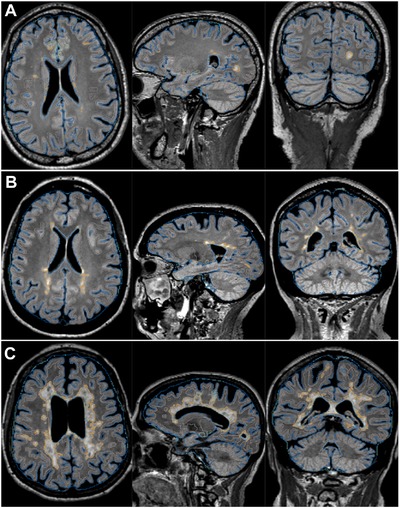
Example segmentations for 3 patients with multiple sclerosis with mild (A), moderate (B), and severe lesion burden (C), respectively. Image planes from left to right represent axial, sagittal, and coronal views. Lesion and cerebrospinal fluid segmentations are shown as orange and blue outlines, respectively.

Figure 2.

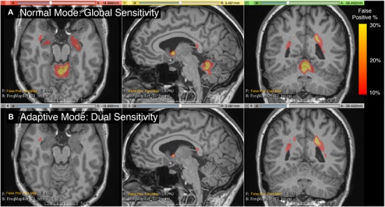
Frequency map of false positives from 20 randomly selected subjects, overlaid on the T1 of a single subject selected as reference. The color overlay shows the frequency of false positive lesions segmented by the automated pipeline. A = normal mode, B = dual sensitivity. A significant reduction in false positive white matter lesions (WMLs) is apparent for the infratentorial region. While infratentorial WMLs accounted for less than 5% of the total lesion burden, this region was responsible for up to 80% (mean 16 ± 19%) of all the false positives (Table 6).

A direct comparison between manual (expert) and automated (3TM) segmentation is shown in Figure 3. The scan‐rescan precision was high for measurements of all segmented tissue classes (WM, GM, CSF, WML, and ICVs) as well as derived BPF metrics, as shown in Bland‐Altman plots in Figure 4. The scan‐rescan experiment yielded coefficients of variation (COVs) of 8% and .4% for automated WMLs and BPF and COVs of .8%, 1%, and 2% for GM, WM, and CSF volumes, respectively. Absolute WML volume difference/precision was .49 ± .72 mL over a WML range of 0–24 mL. Relations between manual and automated WML volume and disease duration as well as EDSS are shown in Figure 5. Relations between manual and automated BPF and disease duration as well as EDSS are shown in Figure 6. Direct correlation between age and 3TM‐derived BPF was r = .62 (n = 29, P = .0004) and r = .58 (P = .001) for automated and manually derived BPF, respectively. Group comparisons between WML volume and BPF for clinical subtypes are shown in Figure 7. The cohort was too small and unbalanced with respect to clinical subgroups to reach significant power, but trends are discernible. WML volumes and BPF for the clinical subgroups were not significantly different between manual and automated methods. Effect size for detecting brain atrophy via automated BPF was d = 1.26 for the entire cohort (29 MS and 15 HC) and d = 1.04 for age‐matched cohorts (23 MS and 12 HC), respectively. An effect size above .8 is considered large and above 1.2 very large.31, 32 However, this effect size should be interpreted as representative for a cohort with a wide range of disease burden as selected here, and not necessarily generalizable to a random sample. A group comparison between the 29 patients with MS and 15 healthy controls is shown in Figure 8. Many standard metrics of segmentation performance are sensitive to the size of objects compared; hence, cases with lower WML burden tend to be consistently rated lower. This effect is shown in a group comparison of segmentation performance for three categories of WML burden in Figure 9.

Figure 3.

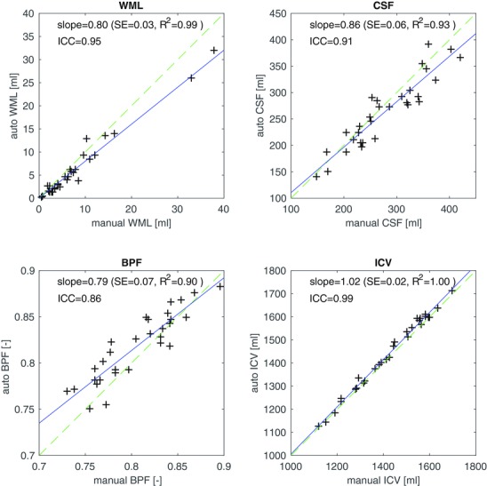
3T morphometry (3TM) segmentation results compared to manual gold standard, for white matter lesion (WML) volume, cerebrospinal fluid (CSF), brain parenchymal fraction (BPF), and total intracranial volume (ICV). The solid (blue) line is a linear regression, and the dashed (green) line represents unity.

Figure 4.

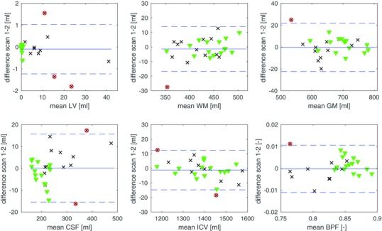
Bland‐Altman plots for the scan‐rescan experiment, in which 15 healthy volunteers (green triangles) and 13 patients with multiple sclerosis (MS) (black x) were scanned twice. The plots show the precision of the automated unedited segmentation for total volumes of white matter (WM), WM lesions volume (LV), gray matter (GM), cerebrospinal fluid (CSF), total intracranial volume (ICV), and brain parenchymal fraction (BPF).

Figure 5.

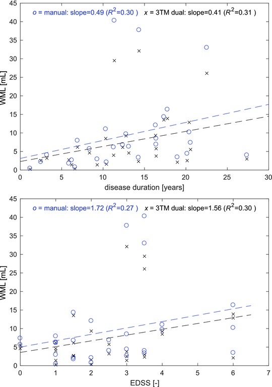
Relationship between white matter lesions (WML) volume and disease duration (top) and Expanded Disability Status Scale (EDSS) score (bottom). x (black) = Automated 3T morphometry (3TM) segmentation, o (blue) = manual WML segmentation. Dashed lines show linear regression fits for both methods.

Figure 6.

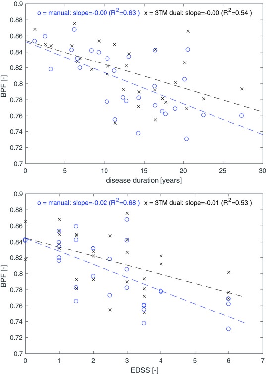
Relationship between brain parenchymal fraction (BPF) and disease duration (top) and Expanded Disability Status Scale (EDSS) score (bottom). x (black) = Automated 3T morphometry (3TM) segmentation, o (blue) = manual white matter lesion segmentation. Dashed lines show linear regression fits for both methods.

Figure 7.

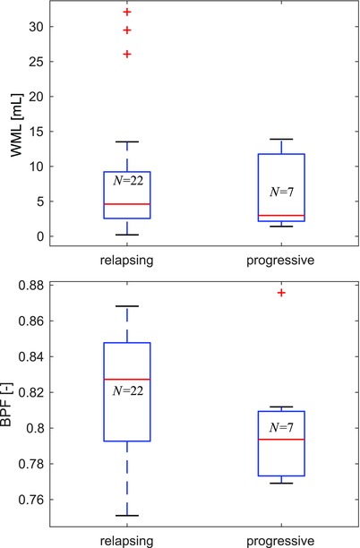
Group comparison of automated MRI segmentation results between relapsing (pooled clinically isolated syndrome + relapsing‐remitting, n = 22) and progressive (pooled primary progressive + secondary progressive, n = 7) multiple sclerosis (MS) subtypes. Trends for higher disease severity (lower BPF) in progressive MS are discernible, but not statistically significant (P > .1) perhaps due to the small and unbalanced cohort. Only the results of automated segmentation are shown; the automated and manual metrics did not differ significantly for the relapsing and progressive subgroups. BPF = brain parenchymal fraction; N = number of patients.

Figure 8.

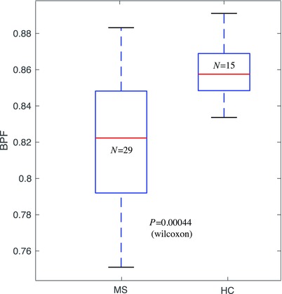
Effect size for detecting atrophy in multiple sclerosis (MS) via the automated brain parenchymal fraction (BPF) measure. Group comparison between patients with MS and healthy controls (HC) yields P < .001 (Wilcoxon). Effect size estimate (Cohen's d) was d = 1.26 (standardized mean difference)31 for the entire cohort (29 MS and 15 HC) and d = 1.04 for age‐matched cohorts.

Figure 9.

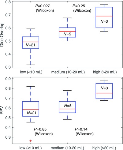
Comparison of performance metrics (manual vs. automated) over the spectrum of disease burden. The cohort was grouped/stratified into WML volume categories of low (less than 10 mL), medium (10‐20 mL), and high (more than 20 mL). Relative metrics, such as Dice or Jaccard, become unstable as objects become smaller and their size approaches a single voxel. Accordingly, Dice scores for lower disease burden (with smaller lesions) are consistently lower. Other metrics like positive predictive value (PPV) or Hausdorff distance are less sensitive to this effect (bottom plot), but have the opposite problem of being less representative as WML volume increases and lesions become confluent. WML = white matter lesion.

Discussion

A fully automated pipeline for the segmentation of WMLs and CSF from high‐resolution multichannel MRI was presented and validated on a cohort of patients with MS and healthy control subjects. A modular framework enabled high flexibility for implementing a complex, multistep image analysis pipeline that exposes a broad range of algorithmic parameters and enables adaptation by configuration rather than reimplementation. Compared to established, existing methods for measuring morphometric parameters of structural brain damage,6, 7, 8, 10, 11, 12 the presented 3TM pipeline introduces a dual‐sensitivity concept and heuristic priors to provide flexibility in processing heterogeneous MRI datasets. By testing the pipeline on a population of subjects showing a wide range of structural brain abnormalities, we provided evidence of such flexibility while maintaining high accuracy and precision performance.

Lesion filling and probabilistic atlases were not used in the tested implementation, but could easily be integrated into the modular pipeline concept. For example, if relative GM versus WM atrophy is used as an outcome metric, lesion filling approaches have proven beneficial.25 Comparison with manual delineation showed good agreement with a low and fairly consistent bias in the total volume of both CSF and WMLs. Since the overall intraclass correlation with expert segmentation is high (ICC_WML = .95, ICC_CSF = .91), we interpret this bias as mostly a result of differences in the working definitions of “hyperintense WM,” ie, an issue of calibrating contrast between manual and automated methods. Such systematic bias does not affect longitudinal or group comparisons and can be addressed by additional calibration and by post‐hoc methods such as imputation.33

A group comparison of segmentation performance for three categories of WML burden is shown in Figure 9. Overlap metrics, such as Dice, are sensitive to object size and thus show significantly lower scores for low disease burden with smaller lesions. Other metrics like PPV or Hausdorff distance are less sensitive to this effect (bottom plot of Fig 9), but have the opposite problem of being less representative as WML volume increases and lesions become confluent.

A key innovation of our presented workflow is in the dual‐sensitivity approach to detect WMLs. We found that a significant improvement in automated WML segmentation from multichannel MRI can be achieved by a dual‐sensitivity approach that employs a separate intensity model for the infratentorial region (Table 5, Fig 2). Significant reductions in false positives were observed, affording increases in global sensitivity without losing specificity. Because infratentorial lesions have elevated significance in terms of disability and progression prognosis, reliable morphometry of this region is important in routine MRI assessment and individual studies may weigh the sensitivity‐specificity trade‐off differently for this region. The dual‐sensitivity concept can easily be extended to additional regions, approaching a model of WM appearance that changes with anatomical region, in modulation with the MRI acquisition protocol.

The 3TM pipeline includes a configurable and extendable set of heuristic rules (Table 3) to correct for typical misclassifications, based on the combination of location, size, and intensity of anatomical substructures. The main goal of this additional step was to improve accuracy and precision of the tissue class segmentation that serves as the spatial prior for the final EM segmentations. A precise anatomical context is needed for those rules, which we found more reliably obtained from a subject‐specific parcellation than from a probabilistic intersubject atlas alone. The motivation for the emphasis on such a rule set and a precise rather than generic anatomical prior is twofold. First, an intuitive and accessible anatomical rule is difficult to obtain in a purely Euclidian context. Second, intensity‐based segmentation algorithms commonly assume spatially uniform tissue appearance (in both intensity and noise) across the brain, which leads to misclassifications where contrast and noise characteristics vary across different regions. This effect, exacerbated at higher MRI field strengths, is also more readily modeled in an anatomical rather than a Euclidian context.

Among the limitations of our work is that the 3TM pipeline was validated only on high‐resolution 3T MRI. However, the basic elements are also applicable to 1.5T MRI, and preliminary tests showed promising results (not shown). Validation also lacks longitudinal data to assess the sensitivity to WML change or progression of atrophy via direct volumetry. Similar to other WML segmentation methods, the 3TM approach relies heavily on the FLAIR image for dissociating the intensity characteristics of WMLs from normal appearing WM and also for defining the heuristic rule set (Table 3). In the absence of an FLAIR image, such rules need to be reconfigured to use a different contrast, such as a proton density or T2‐based series, and would likely require an additional rule to curb false positive WMLs from partial volume effects of the CSF. Similarly, the use of the Freesurfer parcellation27 can be substituted by another tissue class segmentation or anatomical parcellation.

The presented dual‐sensitivity approach departs from the assumption that individual lesions represent independent measurements with a constant error, as the raw measurement sensitivity now varies across the image and introduces a deliberate regional bias. However, in its current form of discrete anatomical regions rather than unconstrained spatial priors, such bias is more readily addressed in statistical analysis. To the extent that the segmentation is to be reviewed and corrected by a manual operator, the adjustment represents a mere efficiency tool to reduce the number of false positives that need be edited by the operator.

We conclude that the presented 3TM pipeline is a reliable tool to perform quantitative analysis of clinically relevant MRI correlates of brain damage in patients with MS. The high accuracy and precision of the measurements across a broad range of disease burden, and the inherent flexibility and intuitive parameter tuning provide a fully automated workflow for the analysis of large and heterogeneous sets of MRI data in large clinical studies.

References

- 1. Confavreux C, Vukusic S. The clinical epidemiology of multiple sclerosis. Neuroimaging Clin N Am 2008;18:589‐622. [DOI] [PubMed] [Google Scholar]
- 2. Weiner HL. The challenge of multiple sclerosis: how do we cure a chronic heterogeneous disease? Ann Neurol 2009;65:239‐48. [DOI] [PubMed] [Google Scholar]
- 3. Kim G, Chu R, Yousuf F, et al. Sample size requirements for one‐year treatment effects using deep gray matter volume from 3T MRI in progressive forms of multiple sclerosis. Int J Neurosci 2017;127:971‐80. [DOI] [PubMed] [Google Scholar]
- 4. Polman CH, Reingold SC, Banwell B, et al. Diagnostic criteria for multiple sclerosis: 2010 revisions to the McDonald criteria. Ann Neurol 2011;69:292‐302. [DOI] [PMC free article] [PubMed] [Google Scholar]
- 5. Filippi M, Rocca MA, Arnold DL, et al. EFNS guidelines on the use of neuroimaging in the management of multiple sclerosis. Eur J Neurol 2006;13:313‐25. [DOI] [PubMed] [Google Scholar]
- 6. Schmidt P, Gaser C, Arsic M, et al. An automated tool for detection of FLAIR‐hyperintense white‐matter lesions in multiple sclerosis. Neuroimage 2012;59:3774‐83. [DOI] [PubMed] [Google Scholar]
- 7. Datta S, Narayana PA. A comprehensive approach to the segmentation of multichannel three‐dimensional MR brain images in multiple sclerosis. Neuroimage Clin 2013;2:184‐96. [DOI] [PMC free article] [PubMed] [Google Scholar]
- 8. Shiee N, Bazin PL, Ozturk A, et al. A topology‐preserving approach to the segmentation of brain images with multiple sclerosis lesions. Neuroimage 2010;49:1524‐35. [DOI] [PMC free article] [PubMed] [Google Scholar]
- 9. Jain S, Sima DM, Ribbens A, et al. Automatic segmentation and volumetry of multiple sclerosis brain lesions from MR images. Neuroimage Clin 2015;8:367‐75. [DOI] [PMC free article] [PubMed] [Google Scholar]
- 10. Van Leemput K, Maes F, Vandermeulen D, et al. Automated segmentation of multiple sclerosis lesions by model outlier detection. IEEE Trans Med Imaging 2001;20:677‐88. [DOI] [PubMed] [Google Scholar]
- 11. Wei X, Warfield SK, Zou KH, et al. Quantitative analysis of MRI signal abnormalities of brain white matter with high reproducibility and accuracy. J Magn Reson Imaging 2002;15:203‐9. [DOI] [PubMed] [Google Scholar]
- 12. Wu Y, Warfield SK, Tan IL, et al. Automated segmentation of multiple sclerosis lesion subtypes with multichannel MRI. Neuroimage 2006;32:1205‐15. [DOI] [PubMed] [Google Scholar]
- 13. Wells WM, Grimson WL, Kikinis R, et al. Adaptive segmentation of MRI data. IEEE Trans Med Imaging 1996;15:429‐42. [DOI] [PubMed] [Google Scholar]
- 14. Garcia‐Lorenzo D, Prima S, Arnold DL, et al. Trimmed‐likelihood estimation for focal lesions and tissue segmentation in multisequence MRI for multiple sclerosis. IEEE Trans Med Imaging 2011;30:1455‐67. [DOI] [PMC free article] [PubMed] [Google Scholar]
- 15. Anbeek P, Vincken KL, van Bochove GS, et al. Probabilistic segmentation of brain tissue in MR imaging. Neuroimage 2005;27:795‐804. [DOI] [PubMed] [Google Scholar]
- 16. Steenwijk MD, Pouwels PJ, Daams M, et al. Accurate white matter lesion segmentation by k nearest neighbor classification with tissue type priors (kNN‐TTPs). Neuroimage Clin 2013;3:462‐9. [DOI] [PMC free article] [PubMed] [Google Scholar]
- 17. Garcia‐Lorenzo D, Francis S, Narayanan S, et al. Review of automatic segmentation methods of multiple sclerosis white matter lesions on conventional magnetic resonance imaging. Med Image Anal 2013;17:1‐18. [DOI] [PubMed] [Google Scholar]
- 18. Horsfield MA, Bakshi R, Rovaris M, et al. Incorporating domain knowledge into the fuzzy connectedness framework: application to brain lesion volume estimation in multiple sclerosis. IEEE Trans Med Imaging 2007;26:1670‐80. [DOI] [PubMed] [Google Scholar]
- 19. Keshavan A, Paul F, Beyer MK, et al. Power estimation for non‐standardized multisite studies. Neuroimage 2016;134:281‐94. [DOI] [PMC free article] [PubMed] [Google Scholar]
- 20. Chu R, Hurwitz S, Tauhid S, et al. Automated segmentation of cerebral deep gray matter from MRI scans: effect of field strength on sensitivity and reliability. BMC Neurol 2017;17:172. [DOI] [PMC free article] [PubMed] [Google Scholar]
- 21. World Medical Association . WMA Declaration of Helsinki ‐ ethical principles for medical research involving human subjects. Available at: www.wma.net/policies-post/wma-declaration-of-helsinki-ethical-principles-for-medical-research-involving-human-subjects/. Accessed November 12, 2017. [Google Scholar]
- 22. Johnson H, Harris G, Williams K. BRAINSFit: mutual information registrations of whole‐brain 3D images, using the insight toolkit. Insight J. Available at: http://hdl.handle.net/1926/1291. Accessed November 12, 2017. [Google Scholar]
- 23. Smith SM. Fast robust automated brain extraction. Hum Brain Mapp 2002;17:143‐55. [DOI] [PMC free article] [PubMed] [Google Scholar]
- 24. Ceccarelli A, Jackson JS, Tauhid S, et al. The impact of lesion in‐painting and registration methods on voxel‐based morphometry in detecting regional cerebral gray matter atrophy in multiple sclerosis. AJNR Am J Neuroradiol 2012;33:1579‐85. [DOI] [PMC free article] [PubMed] [Google Scholar]
- 25. Valverde S, Oliver A, Llado X. A white matter lesion‐filling approach to improve brain tissue volume measurements. Neuroimage Clin 2014;6:86‐92. [DOI] [PMC free article] [PubMed] [Google Scholar]
- 26. Dell'Oglio E, Ceccarelli A, Glanz BI, et al. Quantification of global cerebral atrophy in multiple sclerosis from 3T MRI using SPM: the role of misclassification errors. J Neuroimaging 2015;25:191‐9. [DOI] [PMC free article] [PubMed] [Google Scholar]
- 27. Fischl B, Salat DH, Busa E, et al. Whole brain segmentation: automated labeling of neuroanatomical structures in the human brain. Neuron 2002;33:341‐55. [DOI] [PubMed] [Google Scholar]
- 28. Zijdenbos AP, Dawant BM, Margolin RA, et al. Morphometric analysis of white matter lesions in MR images: method and validation. IEEE Trans Med Imaging 1994;13:716‐24. [DOI] [PubMed] [Google Scholar]
- 29. Dice LR. Measures of the amount of ecologic association between species. Ecology 1945;26:297‐302. [Google Scholar]
- 30. Bland JM, Altman DG. Statistical methods for assessing agreement between two methods of clinical measurement. Lancet 1986;1:307‐10. [PubMed] [Google Scholar]
- 31. Cohen J. Statistical Power Analysis for the Behavioral Sciences. Hillsdale, NJ: Lawrence Erlbaum Associates, 1988. [Google Scholar]
- 32. Sawilowsky S. New effect size rules of thumb. J Mod Appl Stat Methods 2009;8:597‐9. [Google Scholar]
- 33. Chua AS, Egorova S, Anderson MC, et al. Using multiple imputation to efficiently correct cerebral MRI whole brain lesion and atrophy data in patients with multiple sclerosis. Neuroimage 2015;119:81‐8. [DOI] [PubMed] [Google Scholar]
- 34. Tustison NJ, Avants BB, Cook PA, et al. N4ITK: improved N3 bias correction. IEEE Trans Med Imaging 2010;29:1310‐20. [DOI] [PMC free article] [PubMed] [Google Scholar]
- 35. Meier DS, Guttmann CR. Time‐series analysis of MRI intensity patterns in multiple sclerosis. Neuroimage 2003;20:1193‐209. [DOI] [PubMed] [Google Scholar]