Sample size determination for a matched-pairs study with incomplete data by using exact approach

Abstract

This research was motivated by a clinical trial design for a cognitive study. The pilot study was a matched-pairs design where some data are missing, specifically the missing data coming at the end of the study. Existing approaches to determine sample size are all based on asymptotic approaches (e.g., the GEE approach). When the sample size in a clinical trial is small to medium, these asymptotic approaches may not be appropriate for use due to the unsatisfactory type I and II error rates. For this reason, we consider the exact unconditional approach to compute the sample size for a matched-pairs study with incomplete data. Recommendations are made for each possible missing pattern by comparing the exact sample sizes based on three commonly used test statistics, with the existing sample size calculation based on the GEE approach. An example from a real surgeon-reviewers study is used to illustrate the application of the exact sample size calculation in study designs.

1 Introduction

The Alzheimer’s Disease Cooperative Study (ADCS) initiated a Prevention Instrument (PI) project to investigate the cognitive and functional change for elderly adults over 4 years (Cummings et al., 1994, 2006; Banks & Weintraub, 2009; Banks et al., 2014; Bernick & Banks, 2013; Ferris et al., 2006). This is a longitudinal study with a total of 644 cognitively healthy elderly participants who were initially enrolled. These participants were randomized to receive experimental instruments either at home within 2 weeks of their clinic visit or during the clinic visit. In the end, 417 participants completed the study. The missing rate at the end of the study is calculated to be (644 − 417)/644 = 35%, and this missing data is the result of participants lost to follow up. In this ADCS-PI project, six domains were assessed: cognition, behavior, activities of daily living, global change, pharmacoeconomics, and quality of life (Banks et al., 2014). The Clinical Dementia Rating (CDR) is a five-point scale that is often used to quantify the severity of dementia symptoms in the cognition domain: 0=normal, 0.5=very mild dementia, 1=mild dementia, 2=moderate dementia, and 3=severe dementia (Cummings et al., 1994; Banks et al., 2014). The CDR value of zero is used as the threshold to classify the participants as either normal or abnormal at baseline and at the end of the ADCS-PI project. This study has 417 complete samples and 227 incomplete samples with measurements at baseline only.

A general study of the aforementioned dementia example would be a matched-pairs study with incomplete data at baseline or at the end of the study. Matched-pairs studies are often important and popularly adopted in clinical research due to a lack of large numbers of potential participants. This design allows for more confidence in results by removing much of the variation between the two groups, allowing for meaningful clinical studies with smaller participant pools (Xu et al., 2011; Maust et al., 2014). In many cases the outcome measure may be binary, such as mild cognitive impairment vs. dementia, or obese vs. non-obese, institutionalization vs. mortality. Being able to account for missing data points in such studies is important in understanding the disease, especially in rare diseases.

Choi and Stablein (1982) were among the first to identify this practical problem and investigated seven test statistics with regards to type I error control based on simulation studies. These tests include the commonly used McNemar test (McNemar, 1947) by using complete pairs only, the likelihood ratio test, and the test based on the unbiased estimators for the marginal proportions. Tang and Tang (2004) introduced the exact unconditional approach for statistical inference based on the two test statistics recommended by Choi and Stablein (1982) when the sample size is relatively small (no more than 40 in total), for data with missing completely at random. Later, Lin et al. (2009) proposed a new p-value calculation from a Bayesian perspective for a matched-pairs study with missing data.

Recently, Zhang, Cao, and Ahn (2015) developed a new closed-form sample size formula based on the GEE approach for a matched-pairs study with incomplete data. Their simulation studies showed that the nominal power level is controlled well, but the type I error rate could be inflated or conservative in some cases. To overcome the unsatisfactory performance of the error rate control, we propose using the exact unconditional approach based on maximization for sample size determination. Under the unconditional framework, the tail probability is a function of two nuisance parameters for this data, and the p-value is computed as the worst case scenario over the two-dimensional parameter space. We use an improved version of the centroid algorithm by Benke and Skinner (1991) to search for the p-value. Three different test statistics are used in conjunction with the exact unconditional approach for the sample size calculation. We make our recommendations after extensive numerical studies.

The remainder of this article is organized as follows. In Section 2, we introduce the problem in a general case that allows missing data either at baseline or at the end of the study, we then review the existing sample size calculation based on the GEE approach. After that, we present the detailed sample size calculation by using the exact unconditional approach based on three different test statistics. In Section 3, first we numerically compare the sample sizes by using the exact approach and the GEE approach, we then use a real example from a surgeon-reviewer study to illustrate the application of these approaches. In Section 4, we provide some remarks for comparing two paired proportions with missing data.

2 Methods

In a matched-pairs study (e.g., a study in which each participant is measured at baseline and at the end of the study (Type 1 study), or each participant is assessed by two experts (Type 2 study)), the data can be expressed as (X_i1, X_i2) for the i-th participant in the study. In practice, it is possible that some participants miss one of the two measurements (X_i1 or X_i2 could be missing), and others have complete data. We use the Type 1 study to introduce the problem. Suppose N, B, and A are the the numbers of subjects with complete samples (X_i1, X_i2), incomplete samples at baseline only (X_i1,.), and incomplete samples at the end of the study only (., X_i2), respectively. Then the total number of subjects is M = N + A + B. For a study with binary outcomes, let S be the outcome from the study with S = 1 for a positive result and S = 0 for a negative result, see Table 1 for the data structure.

Table 1.

Data for a matched-pairs study with incomplete data

Complete pairs
		After		Total
		S = 1	S = 0
Before	S = 1	n11	n10	n1+(p0)
	S = 0	n01	n00	n0+
Subtotal		n+1(p1)	n+0	N
Incomplete samples
		S = 1	S = 0
Before only		b1	b0	B
After only		a1	a0	A

Let p₀ = n₁₊/N and p₁ = n₊₁/N be the probability of S = 1 at baseline and at the end of the study, respectively. In such studies, it is often assumed that the probability of the response rate is consistent between the complete samples and incomplete samples: $p_0=\frac{b_1}{B}$, and $p_1=\frac{a_1}{A}$. We are interested in testing the following hypotheses

$$H_0:p_0=p_1\text{against}{H}_a:p_0\ne p_1.$$

Zhang et al. (2015) used the GEE approach to compute the sample size when comparing two paired proportions with incomplete data. To attain the pre-specified power 1−β at the significance level of α, the closed-form sample size formula for a given design parameter (p₀, p₁, ρ, q₀, q₁) is presented as

$$M_{\mathit{GEE}}=\frac{[q_0{p}_0(1-p_0)+q_1{p}_1(1-p_1)-2(q_0+q_1-1)\rho p_0(1-p_0)p_1(1-p_1)]{(z_{1-\alpha /2}+z_{1-\beta })}^2}{q_0{q}_1{p}_0(1-p_0)p_1(1-p_1){\left[\mathit{log}\left(\frac{p_1}{1-p_1}/\frac{p_0}{1-p_0}\right)\right]}^2},$$ (1)

where ρ is the correlation coefficient with a range from −1 to 1, and q₀ and q₁ are the proportions of subjects who complete their measurements at baseline and at the end, respectively. In the neurological study analyzed by Choi and Stablein (1982), the missing rate is between 5% and 20%. In the recent work by Zhang et al. (2015) to compute the sample size for a colorectal cancer prevention outreach program, a 20% missing rate is assumed for before or after the intervention. The total missing rate is 40% in their study as assumed. In the aformentioned ADCS study, the missing rate is around 35% (Banks et al., 2014). When (q₀, q₁) = (1, 1), this is a complete study without any missing data, and this missing pattern is considered for reference in our later numerical studies.

The sample size calculation by using the GEE approach in Equation (1) is based on the limitation distribution of the standardized test statistic, which is the GEE parameter estimate divided by its associated asymptotic standard error. This sample size calculation performs well when M goes to +∞. When the required sample size for a study is from small to medium, the sample size calculation based on the GEE approach may not be accurate. In other words, the calculated sample size, M_GEE, could be over- or under-estimated. When M_GEE is under-estimated, a study could fail due to insufficient participants. When it is over-estimated, a longer time for a project is needed in order to address the research questions from the project, and the cost of the project is increased accordingly. For these reasons, we develop a new exact sample size calculation for comparing two paired proportions with incomplete data. The incomplete data is often due to technique issues, such as administration problems (Tang & Tang, 2004), not related to the disease status. For this reason, the missing mechanism is assumed to be missing completely at random in this article.

Exact unconditional approach is often used in conjunction with an existing test statistic to order the sample space to determine the rejection region. Among the two test statistics recommended by Choi and Stablein (1982), under the exact unconditional framework (Tang & Tang, 2004), the test statistic T_c in Equation (2) is more powerful than the other when N is relatively larger than B and A which is often the case in practice. This test statistic is expressed as,

$$T_c=\frac{(B+A)\frac{A{b}_1-B{a}_1}{\sqrt{(b_1+a_1)(B+A-b_1-a_1)}}\sqrt{\frac{(B+A)}{BA}}+2N\frac{n_{10}-n_{01}}{\sqrt{n_{10}+n_{01}}}}{\sqrt{{(B+A)}^2+{(2N)}^2}}.$$ (2)

The test statistic T_c combines the test statistics for comparing the proportions when only the complete pairs are used or only the incomplete samples are used. Under the null hypothesis, T_c asymptotically follows the standard normal distribution (Choi & Stablein, 1982). If the asymptotic distribution under the alternative with p₀ ≠ p₁ can be found, then the sample size can be determined from these two asymptotic distributions. We do not find the alternative asymptotic distribution in existing literature. In addition, sample size calculation based on asymptotic distributions may not be reliable due to unsatisfactory type I and II error control, especially when the sample size is not that large.

For this reason, we consider the exact unconditional approach based on maximization to compute sample size for comparing two paired proportions with missing data. In this unconditional framework, all possible sample points are enumerated, given the subtotal sample sizes (N, B, and A), and the complete sample space is presented as

$$\mathrm{\Omega }=\{(n_{10},n_{01},b_1,a_1):0\le n_{10}\le N,0\le n_{01}\le (N-n_{10}),0\le b_1\le B,0\le a_1\le A\}.$$

It should be noted that the test statistic T_c does not depend on n₁₁ and n₀₀ values. In other words, when two samples have the same value of (n₁₀, n₀₁, b₁, a₁), they should have the same test statistic. Since this is a two-sided problem, $T_c^2$ is used to order the sample space Ω. The null hypothesis is rejected for a large $T_c^2$ value.

Let X = (n₁₀, n₀₁, b₁, a₁) be a sample from Ω and x be the observed data from a study. The tail area is defined as

$$\mathrm{\Omega }(\mathbf{x})=\{\mathbf{x}:T_c^2(\mathbf{x})\ge T_c^2(\mathbf{x})\}.$$

Under the null hypothesis with p₀ = p₁ = p, the exact p-value is calculated as

$$P_{\mathit{Exact}}(\mathbf{x})=\underset{0\le {\pi }_{11}\le p\le 1}{\text{max}}{\displaystyle \sum _{\mathbf{x}\in \mathrm{\Omega }(\mathbf{x})}\frac{N!}{n_{01}!n_{10}!n_{11}!(N-n_{01}-n_{10}-n_{11})!}{(p-{\pi }_{11})}^{n_{01}+n_{10}}{\pi }_{11}^{n_{11}}{(1-2p+{\pi }_{11})}^{(N-n_{01}-n_{10}-n_{11})}\times \frac{B!}{b_1!(B-b_1)!}\frac{A!}{a_1!(A-a_1)!}{p}^{b_1+a_1}{(1-p)}^{B+A-a_1-b_1},}$$

where π₁₁ = P (X_i1 = 1, X_i1 = 1). This exact p-value is computed by maximizing the tail probability over the two nuisance parameters π₁₁ and p, with a range of 0 ≤ π₁₁ ≤ p ≤ 1. In order to search for the global maximum of the tail probability over the two nuisance parameters, the search algorithm proposed by Benke and Skinner (1991) is utilized to find the global maximum. This is an iterative algorithm that averages random perturbations in estimating the nuisance parameters. Specifically, we use this efficient search algorithm with 200 iterations. We calculate the results from the first 100 iterations and the remaining 100 iterations. If they have the same results, the maximum is considered as the global maximum. Otherwise, an additional 100 iterations will be conducted to confirm the global maximum.

To search for the required sample size to attain the pre-specified power (e.g., 1 − β = 80%) at the significance level of α = 0.05 by using the exact approach, we start with a relatively small sample size whose power is below 1 − β. We found that 75% of the sample size formula in Equation (1) given by Zhang et al. (2015), is often small enough with power being lower than 1 − β for the cases studied in this article. In the case that power is still over 1 − β, one can further reduce the sample size until the power at that sample size is lower than 1 − β. Suppose the initial sample size is M₀. The sample sizes for complete and incomplete samples are

$$B=[M_0(1-q_1)],A=[M_0(1-q_0)],\text{and}N=M_0-B-A,$$

where [e] is the largest integer that is less than or equal to e. To compute the power of a study with the sample size M₀, the tail set at the significant level of α should be calculated first. The tail set is defined as the largest set of Ω(x) such that the type I error is guaranteed

$$P_{\mathit{Exact}}(\mathbf{x})\le \alpha .$$

Once the tail set is obtained, the power of the study under the alternative with p₀ ≠ p₁ is calculated as

$${\displaystyle \sum _{\mathbf{x}\in \mathrm{\Omega }(\mathbf{x})}\frac{N!}{n_{01}!n_{10}!n_{11}!(N-n_{01}-n_{10}-n_{11})!}{(p_1-{\pi }_{11})}^{n_{01}}{(p_0-{\pi }_{11})}^{n_{10}}{\pi }_{11}^{n_{11}}{(1-p_0-p_1+{\pi }_{11})}^{(N-n_{01}-n_{10}-n_{11})}\times \frac{B!}{b_1!(B-b_1)!}{p}_0^{b_1}{(1-p_0)}^{B-b_1}\frac{A!}{a_1!(A-a_1)!}{p}_1^{a_1}{(1-p_1)}^{A-a_1},}$$

where ${\pi }_{11}=\rho \sqrt{p_0(1-p_0)p_1(1-p_1)}+p_0{p}_1$ is calculated from the correlation coefficient of a bivariate distribution (Choi & Stablein, 1982). If the power is less than 1 − β, the total sample size is then increased by 1, and the tail set and the power are calculated again under the new sample size M₀ + 1. This procedure is continued until the power is over 1 − β. The total sample size from the last iteration is the required sample size to attain 1 − β power based on the exact approach.

It should be noted that the test statistic, T_c, in Equation (2), can be used to test the data with q₀ < 1 and q₁ < 1. When q₀ = 1 and q₁ = 1, this is a study with complete pairs without any missing data, the McNemar test statistic (McNemar, 1947),

$$T_{MC}=\frac{{(n_{10}-n_{01})}^2}{n_{10}+n_{01}},$$

can be used to compute the exact sample size. Recently, Shan and Zhang (2016) compared the exact sample sizes with the existing asymptotic sample size calculations by Borkhoff, Johnston, Stephens, and Atenafu (2015) based on the asymptotic unconditional McNemar approach, and the GEE approach by using a Wald test statistic (GEE-W) (Pan, 2001). They found that the exact unconditional approach often needs less participants as compared to the GEE-W approach. This research is an important practical extension of their work on exact sample size calculation for complete data to data with incomplete samples when two paired proportions are compared.

In the case with the missing patterns of (q₀ < 1, q₁ = 1) or (q₀ = 1, q₁ < 1), for simplicity, the McNemar test statistic can be used to order the sample space for p-value and power calculations. In this article, we are interested in a study with the missing pattern of (q₀ = 1, q₁ < 1) instead of (q₀ < 1, q₁ = 1) for two reasons: we expect the results from the second missing pattern to be similar to the first missing pattern q₀ = 1 and q₁ < 1; it is very rare for a study to have missing data at baseline but complete data at the end. For a study with the missing pattern of (q₀ = 1, q₁ < 1), a test statistic proposed by Choi and Stablein (1982) can be used, which is

$$T_u=\frac{{\left(\frac{n_{10}+n_{11}+z}{N+B}-\frac{n_{01}+n_{11}}{N}\right)}^2}{\frac{(N-n_{10}-n_{11})(n_{10}+n_{11}){\phi }^2}{N^3}+\frac{(N-n_{10}-n_{11})(n_{01}+n_{11})}{N^3}-\frac{2(n_{00}{n}_{11}-n_{10}{n}_{01})\phi }{N^3}+\frac{b_1(B-b_1){(1-\phi )}^2}{B^3}},$$

where φ = N/(N + B). In this test statistic, $\frac{n_{10}+n_{11}+z}{N+B}$ and $\frac{n_{01}+n_{11}}{N}$ are the unbiased estimates of p₀ and p₁. A general version of T_u can be used for data with missing at baseline or at the end of a study. That test statistic was compared with T_c under the exact unconditional framework, and the results showed that the exact approach based on the general version of T_u is generally not as powerful as that based on the combined test T_c (Tang & Tang, 2004). For this reason, we use T_c for sample size calculation when the incomplete data occurs at baseline or at the end of a study. For the data with missing at the end of a study only, both T_u and T_MC can be used for sample size calculation, and they are compared in the numerical study section.

3 Numerical study

The GEE approach and the proposed exact approach are compared at various p₀, p₁, and ρ to attain 80% power at the significance level of α = 0.05. The correlation coefficients ρ = −0.2, 0, 0.2, 0.4, and 0.6 are studied. Three p₀ values are investigated: 20%, 30%, and 50%, and multiple response rate differences Δ = p₁ − p₀ are studied: 15%, 20%, 25%, and 30%. We consider 6 missing patterns:

$$Q1:(q_0,q_1)=(1,1),Q2:(q_0,q_1)=(0.9,0.7),Q3:(q_0,q_1)=(0.8,0.8),Q4:(q_0,q_1)=(0.7,0.9),Q5:(q_0,q_1)=(1,0.6).$$

The missing patterns Q2 to Q4 represent the data with incomplete samples at baseline or at the end of a study. The pattern Q5 is for samples with missing data that occur only at the end of a study. Suissa and Shuster (1991) were the first to compute exact sample sizes for a matched-pairs study with complete data (Q1) by using T_MC as the test statistic for sample space ordering (Lloyd, 2008b; Fagerland, Lydersen, & Laake, 2013; Shan & Wilding, 2014).

We compute the proposed exact sample size, M_Exact, by enumerating all possible samples given the total sample size N for the complete samples, and B and A for the incomplete samples. As was said, there is no simulation involved in determining the sample size. The competitor is the approach based on the GEE approach, M_GEE, with a closed-form sample size formula (Zhang et al., 2015). The actual type I and II error rates of the proposed approach are computed exactly while the GEE approach computes the actual error rates by using simulation studies (Zhang et al., 2015).

We first compare the performance of the GEE approach and the proposed approach with regards to type I error control. In a table of Zhang et al. (2015) (Table 2 of their work), almost half of the cases have the actual type I error rates over the nominal level, and over 25% of the cases have power being less than the desired power, for data with complete samples, or incomplete samples at baseline or at the end of a study. In Table 3, we provide the actual type I error rate of the GEE approach and the proposed approach with three different correlation coefficients: ρ = 0, 0.15, and 0.3, for complete samples (Q1) and incomplete samples at the end (Q5). The actual type I error rate based on the GEE approach and its associated sample size are from Zhang, Cao, and Ahn (2014). The exact sample size and its actual type I error rate are computed by using T_MC as the test statistic for complete samples and T_u for the incomplete samples. It can be seen that the proposed exact approach guarantees the type I error rate while the existing GEE approach does not. The actual type I error rate of the proposed exact approach is always less than or equal to the nominal level, and Table 4 is used to illustrate this property when p₀ = 20%, and p₁ = 45% at the nominal level of α = 0.05. It can be seen that the exact approach preserves the significance level of a test.

Table 2.

Data from a malpractice review study

Complete pairs
		Reviewer 2		Total
		Yes	No
Reviewer 1	Yes	26	1	27
	No	5	18	23
Subtotal		31	19	N = 50
Incomplete samples
		Yes	No
Reviewer 1 only		2	9	B = 11
Reviewer 2 only		4	4	A = 8

Table 3.

Actual type I error rate comparison between the GEE approach and the proposed exact approach at α = 0.05 when p₀ = 20% and p₁ = 40%. Sample sizes are calculated to attain 80% power.

Missing	ρ	MGEE | MExact: sample size (actual type I error rate)
Complete samples (q0, q1) = (1, 1)	0	85 (0.049) | 84 (0.0499)
	0.15	73 (0.054) | 72 (0.0496)
	0.3	61 (0.056) | 58 (0.0478)
Incomplete samples (q0, q1) = (1, 0.6)	0	108 (0.050) | 95 (0.0483)
	0.15	96 (0.048) | 87 (0.0498)
	0.3	83 (0.045) | 72 (0.0498)

M_GEE and the actual type I error rate by using the GEE approach are from Zhang et al. (2014).

Table 4.

Actual type I error rates for the proposed exact approach when p₀ = 20%, and p₁ = 45% at the nominal level of α = 0.05.

Missing Pattern	ρ = −0.2	ρ = 0	ρ = 0.2	ρ = 0.4
Q1	0.0496	0.0477	0.0479	0.0483
Q2	0.0500	0.0500	0.0498	0.0497
Q3	0.0500	0.0494	0.0500	0.0494
Q4	0.0499	0.0500	0.0499	0.0499
Q5	0.0484	0.0491	0.0496	0.0493

Test statistic T_c is used for sample size calculation when the missing patterns are Q2, Q3, or Q4 with missing data at baseline or at the end, and T_MC is used for a study with no missing data, Q1. When the missing data pattern is Q5, T_u and T_MC can be used. In Figure 1, we compare the sample size calculation based on these two test statistics for data with the missing pattern Q5 when p₀ = 20%, p₁ from 35% to 50%, and correlation coefficient ρ from −0.2 to 0.6. For a given response rate p₁, sample size for each ρ is plotted in the figure. The sample size M_Exact(T_u) is less than M_Exact(T_MC) when the point is above the diagonal line. It can be seen that the exact approach based on T_u always needs fewer participants as compared to that based on T_MC when (q₀, q₁) = (1, 0.6) with 40% of subjects having missing data at the end of the study. The exact approach based on T_u performs better than the other when Δ = p₁ − p₀ is small, although these two exact approaches are comparable when Δ is large and ρ is zero or negative. Similar results are observed for other configurations. We would recommend using the exact approach based on T_u for data with the missing pattern Q5, and T_u is used in the following comparison for a study with this missing pattern.

Figure 1.

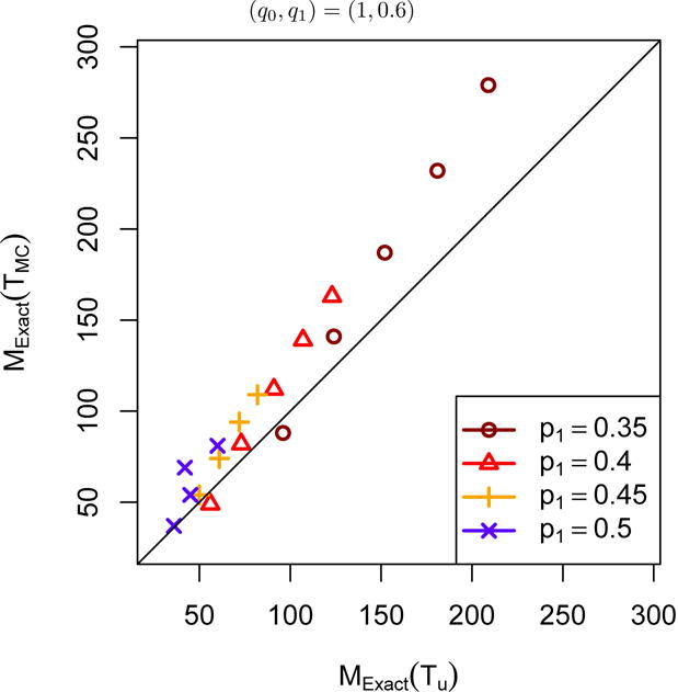
Sample size comparison between M_Exact(T_u) and M_Exact(T_MC) to attain 80% power at α = 0.05 when p₀ = 20% and p₁ = 35%, 40%, 45%, 50%. The sample size M_Exact(T_u) is less than M_Exact(T_MC) when the point is above the diagonal line.

As suggested by one of the reviewers, alternatively the likelihood ratio (LR) test could be used to order the sample size for exact sample size calculation. For a study with complete data, Lloyd (2008b) found that the LR test and the McNemar test have similar performance with regards to power for such studies with complete data. For this reason, the example size based on these two tests should be close to each other. For a study with missing data either at baseline or at the end of a study, the likelihood function is expressed as

$$L(p_0,p_1,{\pi }_{11})={(p_1-{\pi }_{11})}^{n_{01}}{(p_0-{\pi }_{11})}^{n_{10}}{\pi }_{11}^{n_{11}}{(1-p_0-p_1+{\pi }_{11})}^{(N-n_{01}-n_{10}-n_{11})}{p}_0^{b_1}{(1-p_0)}^{B-b_1}{p}_1^{a_1}{(1-p_1)}^{A-a_1}.$$

Then, the LR test is given as

$$LR=-2\log \frac{{\text{max}}_{0}L(p_0,p_1,{\pi }_{11})}{L({\widehat{p}}_0,{\widehat{p}}_1,{\widehat{\pi }}_{11})},$$

where max₀ L(p₀, p₁, π₁₁) is the maximum likelihood function under the null hypothesis, and $L({\widehat{p}}_0,{\widehat{p}}_1,{\widehat{\pi }}_{11})$ is the maximum of the likelihood function. In general, there is no closed-formula to compute these maximum likelihood functions, and one has to compute them by using iterative methods (Choi & Stablein, 1982). The LR test asymptotically follows a chi-squared distribution with one degree of freedom. For each possible data point, we compute the LR test first. We compare the required sample sizes based on the LR test and the T_c test in Table 5. We also provide the actual type I and II error rates for the exact sample size calculation based on the test statistic T_c and the LR test in this table. Both test statistics are used to order the sample space, and the p-value is then computed by using the exact approach as discussed in the manuscript. Table 5 illustrates that both are exact with type I and II error rates guaranteed. It can be seen that they have similar sample sizes in these cases, although the T_c test can save a few participants in general. Obviously, T_c is easy to use in sample size calculation since it has a closed-formula. For this reason, T_c is recommended for use in sample size determination. The LR test is not used in the following sample size comparisons. Therefore, the proposed approach utilizes T_MC for complete data, T_c for data missing at baseline or at the end of a study, and T_u for missing data at the end of a study.

Table 5.

Exact sample size comparison between M_LR based on the likelihood ratio method and $M_{T_c}$ based on the test statistic T_c for the missing types Q₂, Q₃, and Q₄ to attain 80% power at α = 0.05 when p₀ = 20% and p₁ = 50%.

Missing	$M_{LR}|M_{T_c}$: sample size (actual type I error rate, actual power)
	ρ = 0	ρ = 0.2
Q2	56(0.0499, 0.8091) | 53 (0.0498, 0.8049)	46 (0.04980, 0.8083) | 43 (0.04990, 0.8015)
Q3	55(0.0496, 0.8078) | 51 (0.0500, 0.8039)	47 (0.04990, 0.8171) | 42 (0.05000, 0.8064)
Q4	55(0.0499, 0.8024) | 53 (0.0498, 0.8099)	46 (0.04970, 0.8091) | 43 (0.04970, 0.8050)

We present the sample sizes, M_GEE and M_Exact, for various combinations of p₁ and ρ when p₀ = 20% in Table 6. Under the alternative with p₀ and p₁ as the marginal response rates, the response rate for π₁₁ is calculated as ${\pi }_{11}=\rho \sqrt{p_0(1-p_0)p_1(1-p_1)}+p_0{p}_1$, where 0 < π₁₁ < min(p₀, p₁). We found that π₁₁ is larger than p₀ = 20% when p₁ = 45% or 50%. In these cases, sample size calculations based on the exact approach does not exist. Although one can still use the GEE sample size calculation formula in Equation (1) to compute the required sample size, this may not be practically correct since the estimate of π₁₀ is negative which is not considered a constraint in the GEE sample size calculation.

Table 6.

Sample size comparison between M_GEE and M_Exact to attain 80% power at α = 0.05 when p₀ = 20%.

		MGEE | MExact
p1	Missing	ρ = −0.2	ρ = 0	ρ = 0.2	ρ = 0.4	ρ = 0.6
p1 = 35%	Q1	170 | 168	142 | 140	114 | 113	87 | 86	59 | 53
	Q2	203 | 221	177 | 189	150 | 155	124 | 119	97 | 79
	Q3	204 | 209	178 | 179	152 | 149	126 | 115	99 | 77
	Q4	211 | 217	185 | 186	158 | 153	131 | 119	105 | 78
	Q5	209 | 209	182 | 181	154 | 152	126 | 124	98 | 96
p1 = 40%	Q1	102 | 99	85 | 84	69 | 68	52 | 50	36 | 30
	Q2	122 | 131	106 | 112	90 | 92	74 | 69	58 | 45
	Q3	122 | 124	107 | 105	91 | 88	76 | 68	60 | 44
	Q4	127 | 128	111 | 110	95 | 91	79 | 69	64 | 46
	Q5	125 | 123	108 | 107	91 | 91	75 | 73	58 | 56
p1 = 45%	Q1	69 | 66	58 | 57	47 | 45	36 | 33
	Q2	82 | 86	72 | 75	61 | 61	50 | 46
	Q3	83 | 82	72 | 70	62 | 58	51 | 44
	Q4	86 | 85	75 | 73	65 | 61	54 | 46
	Q5	84 | 82	73 | 72	62 | 61	51 | 50
p1 = 50%	Q1	51 | 49	42 | 42	34 | 33	26 | 23
	Q2	60 | 62	52 | 53	44 | 43	37 | 33
	Q3	60 | 59	53 | 51	45 | 42	38 | 32
	Q4	63 | 61	55 | 53	47 | 43	40 | 33
	Q5	61 | 60	53 | 42	45 | 45	37 | 36

It can be seen in Table 6 that the required sample size generally decreases as the correlation coefficient ρ increases for a given design configuration for both approaches. When the response rate difference, Δ = p₁ − p₀, increases from 15% to 30% as in the table, the sample size is decreased. For a study with the missing pattern Q1 or Q5, M_Exact is always slightly smaller than M_GEE, and the sample size difference between these two approaches is often small. For the other missing patterns from Q2 to Q4, although the exact approach may need more participants in a few configurations with negative or zero correlation, the exact approach generally needs fewer subjects than the GEE approach, and the sample size savings from the exact approach is substantial when ρ is large.

We plot the sample sizes, M_GEE against M_Exact, when p₀ = 30%, p₁ = 50%, and ρ = −0.2 to 0.6, in Figure 2. Similar to the results observed from Table 6, sample size increases as the correlation coefficient ρ goes down from 0.6 to −0.2. The sample size based on the exact approach is smaller than that based on the GEE approach when ρ is large, and this trend is reversed when ρ is small or negative and the missing patterns are Q2 to Q4. Out of the 30 total cases seen in Figure 2, the exact sample size is less than or equal to that based on the GEE approach in the majority of the cases. We also provide the sample size calculation when p₀ = 50% in Table 7. Similar results are observed to these in Table 6 and Figure 2.

Figure 2.

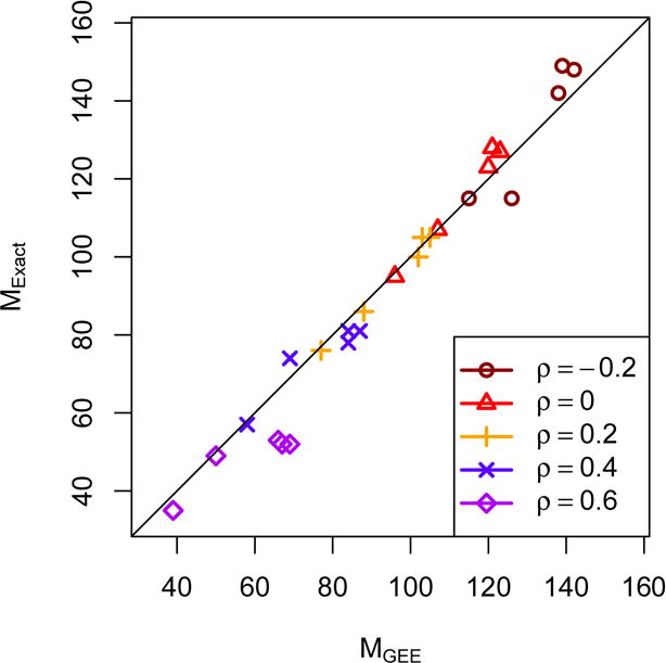
Sample size comparison between M_GEE and M_Exact to attain 80% power at α = 0.05 with ρ from −0.2 to 0.6, when p₀ = 30% and p₁ = 50%. The sample size M_Exact is less than M_GEE when the point is below the diagonal line.

Table 7.

Sample size comparison between M_GEE and M_Exact to attain 80% power at α = 0.05 when p₀ = 50%.

		MGEE | MExact
p1	Missing	ρ = −0.2	ρ = 0	ρ = 0.2	ρ = 0.4	ρ = 0.6	ρ = 0.7
p1 = 65%	Q1	207 | 206	172 | 173	138 | 137	104 | 105	69 | 67	52 | 44
	Q2	253 | 269	220 | 231	187 | 191	155 | 147	122 | 99	106 | 71
	Q3	248 | 258	215 | 222	183 | 184	151 | 143	119 | 97	103 | 69
	Q4	250 | 271	218 | 232	185 | 191	152 | 147	119 | 99	103 | 72
	Q5	267 | 266	232 | 232	198 | 197	164 | 162	129 | 127	112 | 111
p1 = 70%	Q1	115 | 115	96 | 95	77 | 76	58 | 57	39 | 35
	Q2	142 | 148	123 | 127	105 | 105	87 | 81	69 | 53
	Q3	138 | 142	120 | 123	102 | 100	84 | 78	67 | 50
	Q4	139 | 149	121 | 128	103 | 105	84 | 81	66 | 53
	Q5	150 | 147	131 | 130	112 | 111	93 | 92	74 | 71
p1 = 75%	Q1	73 | 72	61 | 61	49 | 49	37 | 36
	Q2	90 | 92	79 | 79	68 | 65	56 | 49
	Q3	88 | 88	76 | 76	65 | 63	54 | 48
	Q4	88 | 93	76 | 79	65 | 65	53 | 49
	Q5	96 | 93	84 | 81	72 | 69	60 | 58

3.1 Examples

We use a real example to illustrate the application of the proposed new exact sample size, M_Exact, as compared to the existing asymptotic sample size, M_GEE. This study involved two surgeon-reviewers who evaluated the 69 cases (Greenberg et al., 2007). They were asked whether ‘hand-offs in care’ was a contributing factor in communication breakdowns. Their answers to each question were either ‘Yes’ or ‘No’. Among these 69 claims, 50 were reviewed by both surgeon-reviewers, and 11 claims were reviewed by reviewer 1 only, and the remaining 8 claims were assessed by reviewer 2 only. The detailed data are given in Table 2. We combine all data to estimate the response rate of ‘Yes’ for each reviewer: p₀ = 29/61 = 47.5% for reviewer 1, and p₁ = 35/58 = 60% for reviewer 2. The missing rates are estimated as q₀ = 80% and q₁ = 85%. We use the complete samples to estimate the correlation coefficient as ρ = 0.75. To attain 80% power at α = 0.05, the GEE sample size is M_GEE = 125, and the proposed exact sample size based on the test statistic T_c is M_Exact = 78. The required sample size by the exact approach is much smaller than the GEE sample size. When the nomial level is increased to α = 0.1, the required sample sizes are M_GEE = 99 and M_Exact = 59, respectively. In the case for a study at α = 0.01, M_GEE = 186 and M_Exact = 122 are required based on the GEE approach and the proposed exact approach.

The difference between these two approaches is relatively large as compared to those in the simulation study. In order to meet the condition that all the probabilities are positive, the upper bound for correlation coefficient ρ is 0.7766. The correlation coefficient is estimated as 0.75 from the example, which is very close to the upper bound. It can be seen from the numerical study that the exact approach saves more sample sizes as compared to the GEE approach when the correlation increases for this type of missing pattern.

4 Discussion

In this article, we developed a new exact sample size calculation for a matched-pairs study with incomplete data. As compared to the exact approach for sample size calculation, (Lloyd, 2007, 2014, 2008a; Shan, 2013; Shan, Ma, Hutson, & Wilding, 2012; Shan & Ma, 2016; Shan, 2015; Shan, Wilding, Hutson, & Gerstenberger, 2016; Shan, Moonie, & Shen, 2016; Shan, 2015), the existing GEE approach does not guarantee type I and II error rates although it is computationally easy with a closed form. With the wide availability of powerful computers or supercomputers, exact sample size computation is practical and feasible. The program to compute exact sample sizes is written in R, (Shan & Wang, 2013), and it is available by request from the first author. The exact sample sizes are recommended for use in practice to improve the effectiveness of a study, and have the potential to increase the success rate of clinical trials with adequate and accurate sample size to attain the pre-specified power.

In this article, we compared the performance of the McNemar test with the test statistics proposed by Choi and Stablein (1982), T_u, by using the exact approach for a study with missing data at the end only (missing pattern Q5). The test statistic T_u uses all data while the McNemar test only uses the complete samples without considering the incomplete samples. The test statistic T_u is often more powerful than T_MC for data with the missing pattern of q₀ = 1 and q₁ < 1, and is associated with fewer participants in general. When data is missing at random or missing not at random, the assumption of response rate consistency between complete data and incomplete data is not valid. Li and Caffo (2011) conducted a simulation study to compare proportions with missing data. They assumed that the missing process is dependent on two covariates in the simulation study. A logistic regression model was used in the simulation study to investigate the robustness of their developed maximum likelihood estimator for a binary outcome. They considered 10 different missing at random scenarios to investigate the results. They found that the performance of their proposed estimator is dependent on the missing scenario. We consider comparing the performance and robustness of the GEE approach and the proposed exact approach in sample size calculation for a matched-pairs study with missing at random or missing not at random, as future work. When the required sample size is large, exact approaches could be computationally intensive, and other approaches based on Monte Carlo simulation (Muthén & Muthén, 2002) or the bootstrap method (Yuan & Hayashi, 2003) could be used.

If different approaches are used in sample size calculation and final data analysis, it is possible that we may fail to reject the null hypothesis given the sufficient sample size calculated from an efficient method in the sample size planning. For this reason, we would highly recommend researchers analyze the final data consistently by using the same approach used in the sample size calculation. In addition to that, researchers should also be encouraged to identify the most appropriate approach for analyzing the data by controlling for other possible confounding factors.

References

- Banks SJ, Raman R, He F, Salmon DP, Ferris S, Aisen P, Cummings J. The Alzheimer’s disease cooperative study prevention instrument project: longitudinal outcome of behavioral measures as predictors of cognitive decline. Dementia and geriatric cognitive disorders extra. 2014;4(3):509–516. doi: 10.1159/000357775. Retrieved from http://view.ncbi.nlm.nih.gov/pubmed/25685141. [DOI] [PMC free article] [PubMed] [Google Scholar]
- Banks SJ, Weintraub S. Generalized and symptom-specific insight in behavioral variant frontotemporal dementia and primary progressive aphasia. The Journal of neuropsychiatry and clinical neurosciences. 2009;21(3):299–306. doi: 10.1176/appi.neuropsych.21.3.299. Retrieved from http://dx.doi.org/10.1176/appi.neuropsych.21.3.299. [DOI] [PMC free article] [PubMed] [Google Scholar]
- Benke KK, Skinner DR. A Direct Search Algorithm for Global Optimisation of Multivariate Functions. Australian Computer Journal. 1991;23(2):73–85. [Google Scholar]
- Bernick C, Banks S. What boxing tells us about repetitive head trauma and the brain. Alzheimer’s Research & Therapy. 2013;5(3):23+. doi: 10.1186/alzrt177. Retrieved from http://dx.doi.org/10.1186/alzrt177. [DOI] [PMC free article] [PubMed] [Google Scholar]
- Borkhoff CM, Johnston PR, Stephens D, Atenafu E. The special case of the 2 2 table: asymptotic unconditional McNemar test can be used to estimate sample size even for analysis based on GEE. Journal of clinical epidemiology. 2015 Jul;68(7):733–739. doi: 10.1016/j.jclinepi.2014.09.025. Retrieved from http://view.ncbi.nlm.nih.gov/pubmed/25510372. [DOI] [PubMed] [Google Scholar]
- Choi SC, Stablein DM. Practical Tests for Comparing Two Proportions with Incomplete Data. (Series C (Applied Statistics)).Journal of the Royal Statistical Society. 1982;31(3):256–262. [Google Scholar]
- Cummings JL, Mega M, Gray K, Rosenberg-Thompson S, Carusi DA, Gornbein J. The Neuropsychiatric Inventory: comprehensive assessment of psychopathology in dementia. Neurology. 1994 Dec;44(12):2308–2314. doi: 10.1212/wnl.44.12.2308. Retrieved from http://view.ncbi.nlm.nih.gov/pubmed/7991117. [DOI] [PubMed] [Google Scholar]
- Cummings JL, Raman R, Ernstrom K, Salmon D, Ferris SH, Alzheimer’s Disease Cooperative Study Group ADCS Prevention Instrument Project: behavioral measures in primary prevention trials. Alzheimer disease and associated disorders. 2006;20(4 Suppl 3) doi: 10.1097/01.wad.0000213872.17429.0f. Retrieved from http://view.ncbi.nlm.nih.gov/pubmed/17135808. [DOI] [PubMed] [Google Scholar]
- Fagerland MW, Lydersen S, Laake P. The McNemar test for binary matched-pairs data: mid-p and asymptotic are better than exact conditional. BMC medical research methodology. 2013 Jul 13;13 doi: 10.1186/1471-2288-13-91. Retrieved from http://view.ncbi.nlm.nih.gov/pubmed/23848987. [DOI] [PMC free article] [PubMed] [Google Scholar]
- Ferris SH, Aisen PS, Cummings J, Galasko D, Salmon DP, Schneider L, Alzheimer’s Disease Cooperative Study Group ADCS Prevention Instrument Project: overview and initial results. Alzheimer disease and associated disorders. 2006;20(4 Suppl 3) doi: 10.1097/01.wad.0000213870.40300.21. Retrieved from http://view.ncbi.nlm.nih.gov/pubmed/17135805. [DOI] [PubMed] [Google Scholar]
- Greenberg CC, Regenbogen SE, Studdert DM, Lipsitz SR, Rogers SO, Zinner MJ, Gawande AA. Patterns of communication breakdowns resulting in injury to surgical patients. Journal of the American College of Surgeons. 2007 Apr;204(4):533–540. doi: 10.1016/j.jamcollsurg.2007.01.010. Retrieved from http://view.ncbi.nlm.nih.gov/pubmed/17382211. [DOI] [PubMed] [Google Scholar]
- Li X, Caffo BS. Comparison of Proportions for Composite Endpoints with Missing Components. Journal of Biopharmaceutical Statistics. 2011 Feb 28;21(2):271–281. doi: 10.1080/10543406.2011.550109. Retrieved from http://dx.doi.org/10.1080/10543406.2011.550109. [DOI] [PMC free article] [PubMed] [Google Scholar]
- Lin Y, Lipsitz S, Sinha D, Gawande AA, Regenbogen SE, Greenberg CC. Using Bayesian p-values in a 2 2 table of matched pairs with incompletely classified data. (Series C, Applied statistics).Journal of the Royal Statistical Society. 2009 May 1;58(2):237–246. doi: 10.1111/j.1467-9876.2008.00645.x. Retrieved from http://view.ncbi.nlm.nih.gov/pubmed/19657473. [DOI] [PMC free article] [PubMed] [Google Scholar]
- Lloyd CJ. Efficient and exact tests of the risk ratio in a correlated 2 × 2 table with structural zero. Computational Statistics & Data Analysis. 2007 May;51:3765–3775. Retrieved from http://portal.acm.org/citation.cfm?id=1234418.1234637. [Google Scholar]
- Lloyd CJ. Exact p-values for discrete models obtained by estimation and maximization. Australian and New Zealand Journal of Statistics. 2008a;50(4):329–345. doi: 10.1111/j.1467-842x.2008.00520.x. Retrieved from http://dx.doi.org/10.1111/j.1467-842x.2008.00520.x. [DOI] [Google Scholar]
- Lloyd CJ. A new exact and more powerful unconditional test of no treatment effect from binary matched pairs. Biometrics. 2008b;64(3):716–723. doi: 10.1111/j.1541-0420.2007.00936.x. Retrieved from http://dx.doi.org/10.1111/j.1541-0420.2007.00936.x. [DOI] [PubMed] [Google Scholar]
- Lloyd CJ. On the exact size of tests of treatment effects in multi-arm clinical trials. Australian and New Zealand Journal of Statistics. 2014 Dec 1;56(4):359–369. doi: 10.1111/anzs.12089. Retrieved from http://dx.doi.org/10.1111/anzs.12089. [DOI] [Google Scholar]
- Maust DT, Kim HM, Seyfried LS, Chiang C, Kavanagh J, Schneider L, Kales HC. Number Needed to Harm for Antipsychotics and Antidepressants in Dementia. The American Journal of Geriatric Psychiatry. 2014 Mar;22(3):S119–S120. doi: 10.1016/j.jagp.2013.12.137. Retrieved from http://dx.doi.org/10.1016/j.jagp.2013.12.137. [DOI] [Google Scholar]
- McNemar Q. Note on the sampling error of the difference between correlated proportions or percentages. Psychometrika. 1947 Jun;12(2):153–157. doi: 10.1007/BF02295996. Retrieved from http://view.ncbi.nlm.nih.gov/pubmed/20254758. [DOI] [PubMed] [Google Scholar]
- Muthén LK, Muthén BO. How to Use a Monte Carlo Study to Decide on Sample Size and Determine Power. Structural Equation Modeling: A Multidisciplinary Journal. 2002 Oct 1;9(4):599–620. doi: 10.1207/s15328007sem0904\_8. Retrieved from http://dx.doi.org/10.1207/s15328007sem0904\_8. [DOI] [Google Scholar]
- Pan W. Sample size and power calculations with correlated binary data. Controlled clinical trials. 2001 Jun;22(3):211–227. doi: 10.1016/s0197-2456(01)00131-3. Retrieved from http://view.ncbi.nlm.nih.gov/pubmed/11384786. [DOI] [PubMed] [Google Scholar]
- Shan G. A Note on Exact Conditional and Unconditional Tests for Hardy-Weinberg Equilibrium. Human Heredity. 2013;76(1):10–17. doi: 10.1159/000353205. Retrieved from http://dx.doi.org/10.1159/000353205. [DOI] [PubMed] [Google Scholar]
- Shan G. Exact Statistical Inference for Categorical Data. 1st. Academic Press; 2015. Paperback. Retrieved from http://www.worldcat.org/isbn/0081006810. [Google Scholar]
- Shan G, Ma C. Unconditional tests for comparing two ordered multinomials. Statistical methods in medical research. 2016 Feb 01;25(1):241–254. doi: 10.1177/0962280212450957. Retrieved from http://dx.doi.org/10.1177/0962280212450957. [DOI] [PubMed] [Google Scholar]
- Shan G, Ma C, Hutson AD, Wilding GE. An efficient and exact approach for detecting trends with binary endpoints. Statistics in Medicine. 2012;31(2):155–164. doi: 10.1002/sim.4411. Retrieved from http://dx.doi.org/10.1002/sim.4411. [DOI] [PubMed] [Google Scholar]
- Shan G, Moonie S, Shen J. Sample size calculation based on efficient unconditional tests for clinical trials with historical controls. Journal of biopharmaceutical statistics. 2016;26(2):240–249. doi: 10.1080/10543406.2014.1000545. Retrieved from http://view.ncbi.nlm.nih.gov/pubmed/25551261. [DOI] [PubMed] [Google Scholar]
- Shan G, Wang W. ExactCIdiff: An R Package for Computing Exact Confidence Intervals for the Difference of Two Proportions. The R Journal. 2013;5(2):62–71. [Google Scholar]
- Shan G, Wilding GE. Powerful Exact Unconditional Tests for Agreement between Two Raters with Binary Endpoints. PLoS ONE. 2014 May 16;9(5):e97386+. doi: 10.1371/journal.pone.0097386. Retrieved from http://dx.doi.org/10.1371/journal.pone.0097386. [DOI] [PMC free article] [PubMed] [Google Scholar]
- Shan G, Wilding GE, Hutson AD, Gerstenberger S. Optimal adaptive two-stage designs for early phase II clinical trials. Statist Med. 2016 Apr 15;35(8):1257–1266. doi: 10.1002/sim.6794. Retrieved from http://dx.doi.org/10.1002/sim.6794. [DOI] [PMC free article] [PubMed] [Google Scholar]
- Shan G, Zhang H. Exact unconditional sample size determination for paired binary data (letter commenting: J Clin Epidemiol. 2015;68:733–739) Journal of Clinical Epidemiology. 2016;78 doi: 10.1016/j.jclinepi.2016.07.018. [DOI] [PubMed] [Google Scholar]
- Suissa S, Shuster JJ. The 2 × 2 matched-pairs trial: exact unconditional design and analysis. Biometrics. 1991 Jun;47(2):361–372. Retrieved from http://view.ncbi.nlm.nih.gov/pubmed/1912252. [PubMed] [Google Scholar]
- Tang ML, Tang NS. Exact Tests for Comparing Two Paired Proportions with Incomplete Data. Biom J. 2004 Feb 1;46(1):72–82. doi: 10.1002/bimj.200210003. Retrieved from http://dx.doi.org/10.1002/bimj.200210003. [DOI] [Google Scholar]
- Xu WL, Atti AR, Gatz M, Pedersen NL, Johansson B, Fratiglioni L. Midlife overweight and obesity increase late-life dementia risk. Neurology. 2011 May 03;76(18):1568–1574. doi: 10.1212/wnl.0b013e3182190d09. Retrieved from http://dx.doi.org/10.1212/wnl.0b013e3182190d09. [DOI] [PMC free article] [PubMed] [Google Scholar]
- Yuan KHH, Hayashi K. Bootstrap approach to inference and power analysis based on three test statistics for covariance structure models. The British journal of mathematical and statistical psychology. 2003 May;56(Pt 1):93–110. doi: 10.1348/000711003321645368. Retrieved from http://view.ncbi.nlm.nih.gov/pubmed/12803824. [DOI] [PubMed] [Google Scholar]
- Zhang S, Cao J, Ahn C. A GEE Approach to Determine Sample Size for Pre- and Post-Intervention Experiments with Dropout. Computational statistics & data analysis. 2014 Jan;69 doi: 10.1016/j.csda.2013.07.037. Retrieved from http://view.ncbi.nlm.nih.gov/pubmed/24293779. [DOI] [PMC free article] [PubMed] [Google Scholar]
- Zhang S, Cao J, Ahn C. Sample size calculation for before-after experiments with partially overlapping cohorts. Contemporary clinical trials. 2015 Sep 28; doi: 10.1016/j.cct.2015.09.015. Retrieved from http://view.ncbi.nlm.nih.gov/pubmed/26416696. [DOI] [PMC free article] [PubMed]