Family of boundary overlap metrics for the evaluation of medical image segmentation

Abstract.

All medical image segmentation algorithms need to be validated and compared, yet no evaluation framework is widely accepted within the imaging community. None of the evaluation metrics that are popular in the literature are consistent in the way they rank segmentation results: they tend to be sensitive to one or another type of segmentation error (size, location, and shape) but no single metric covers all error types. We introduce a family of metrics, with hybrid characteristics. These metrics quantify the similarity or difference of segmented regions by considering their average overlap in fixed-size neighborhoods of points on the boundaries of those regions. Our metrics are more sensitive to combinations of segmentation error types than other metrics in the existing literature. We compare the metric performance on collections of segmentation results sourced from carefully compiled two-dimensional synthetic data and three-dimensional medical images. We show that our metrics: (1) penalize errors successfully, especially those around region boundaries; (2) give a low similarity score when existing metrics disagree, thus avoiding overly inflated scores; and (3) score segmentation results over a wider range of values. We analyze a representative metric from this family and the effect of its free parameter on error sensitivity and running time.

1. Introduction

It is often necessary to evaluate the results of image segmentation (and, indeed, compare contours in general) in an established systematic way. Despite attempts by several authors to classify and analyze methods for evaluating medical image segmentation, this field still lacks a widely accepted evaluation framework.

We propose a new family of boundary overlap metrics which detect and measure a wider range of segmentation errors than are detected by most existing metrics. Throughout this paper we use the term “metric” to refer to an evaluation measure of a segmentation result. Strictly speaking, a metric should be symmetric with respect to its operands, whereas some of the discussed similarity or difference criteria listed below are asymmetric. Existing literature uses both “measure” and “metric” interchangeably,^1–3 but metric is intuitive to a wider audience. Our proposed metrics combine features of both overlap-based metrics and boundary-distance-based metrics in order to assess the similarity or difference of two regions: they do this by analyzing the overlap in boundary neighborhoods. The metrics, therefore, assess the percentage of boundary match between the expected correct shape and the segmentation result.

Empirical discrepancy methods (as per Zhang’s classification⁴) compare segmented images to ground truth by exploring the similarity or difference of the labeled regions. The term “ground truth” describes the reference regions against which segmentations are compared. These reference regions are either generated synthetically or are produced manually by trained human operators. For our synthetic data, the ground truth consists of two-dimensional (2-D) black and white images. For medical data, it is a mask that has been hand-drawn onto 2-D or three-dimensional (3-D) medical scan images. Each metric outputs a score that measures the similarity or difference between the given ground truth and a segmented region. The term “machine segmentation” refers to results obtained automatically, semiautomatically, or even manually.

We consider three common classes of such metrics: overlap-, size-, and boundary-distance-based, and examine the most frequently used members of these classes. These metrics are only sensitive to limited, mostly separate, ranges of segmentation errors; they produce contradictory scores and rankings. Heimann et al.⁵ proposed a framework for combining results from several metrics to produce a single score. Nevertheless, this remains an open question. More recent reports comparing segmentation algorithms avoid this by using one metric as the main indicator of segmentation quality⁶ or by averaging rankings of algorithms obtained with different metrics.⁷

An ideal metric should

• a.be able to flag even minute differences between any machine segmentation and its corresponding ground truth,
• b.be able to flag different types of segmentation errors (size, location, and shape),
• c.spread its scores over much of its domain (say between 0% and 100%),
• d.be usable as a ranking tool for different segmentation algorithms.

We first construct a dataset of 52 synthetic images to simulate segmentation results with varying deviations from a chosen ground truth. We measure these images with a range of evaluation metrics (including our own) and reveal how well these correlate with specific segmentation errors. We subsequently compare the performance of the same metrics on real 3-D scan images, using automatically segmented medical images⁸ and hand-drawn ground truth masks. These experimental results show that our metrics fulfill the above goals.

Based on the results illustrated, we propose a new metric from the boundary overlap family which can be used systematically in assessing the results of segmentation, alongside existing metrics. In the future, our metric family can substitute effectively a number of existing metrics or can be adopted as a single general way of evaluation.

2. Existing Evaluation Methods

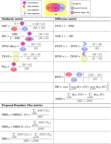
Because there is no agreed upon framework for evaluating the results of segmentation, authors choose their own metrics. In many cases, a metric is chosen because it was used in a prior reference paper with which a newly designed method is being compared. While this enables direct comparison, it also generates a vicious circle which perpetuates the use of less than ideal metrics. Based on our own literature survey,⁹ although new evaluation methods have been proposed,¹⁰ the most popular methods in use in the segmentation literature are still metrics with simple definitions and/or simple descriptions. Their definitions are presented in Fig. 1.

Fig. 1.

(1) Overlap-based: DSC and SVD; JSC and VOE; TPVF, TNVF, FPVF, and FNVF; precision and recall. (2) Size-based: RVD. (3) Boundary-distance-based: HD and ASSD. (4) Our new metric: SBD; its directional variants: ${\mathrm{DBD}}_G$ and ${\mathrm{DBD}}_M$.

2.1. Overlap-Based Methods

2.1.1. Dice similarity coefficient and symmetric volume difference

Originally introduced by Dice¹¹ for ecological studies, the Dice similarity coefficient (DSC) (also known as $F1$ score) is one of the evaluation metrics most frequently used in medical image segmentation.^12–14 Symmetric volume difference (SVD) is a Dice-based error metric which gives the symmetric difference of the segmentation result and the reference shape.^15,16 The term symmetric volume overlap is introduced by Campadelli et al.¹⁷ for $\mathrm{SVO}=1-\mathrm{SVD}$, and is essentially the same as Dice, and used as their main metric.

2.1.2. Jaccard similarity coefficient and volumetric overlap error

The Jaccard similarity coefficient (JSC), used by Liu et al.¹⁸ (presented as similarity ratio), is defined as the intersection between the machine segmentation and the ground truth regions over their union. It is related to DSC, as shown in Fig. 1. Volumetric overlap error (VOE) is the corresponding error metric.^19,20

2.1.3. Volume fractions

Four metrics—true positive (TPVF), true negative (TNVF), false positive (FPVF), and false negative (FNVF) volume fractions—are borrowed from statistical decision theory metrics (sensitivity and specificity).² Only two of the proposed metrics should be used together (e.g., TPVF and FPVF, but not TPVF and FNVF) because of the dependence relationships. Some authors^18,19 give an alternative definition for FPVF by normalizing the number of false-positive voxels over the ground truth rather than the rest of the image. The TPVF–TNVF pair is used by some authors,^21–23 while others^20,24,25 compute the TPVF–FPVF pair.

2.1.4. Precision and recall

Precision normalizes the volume of the correctly segmented region over the volume of the result of the segmentation. Recall (same as TPVF) normalizes the size of the correctly segmented region over the ground truth. Precision does not account for undersegmentation errors, while oversegmentation is not reflected in recall. This pair is used in Refs. ¹³ and ²⁶. It is also used extensively in computer vision.

2.2. Size-Based Methods

2.2.1. Relative volume difference

Relative volume difference (RVD) measures the absolute size difference of the regions, as a fraction of the size of the reference. The metric is sometimes also called relative absolute volume difference. It is used commonly alongside other metrics.^{5,12,19,20,27,28}

2.3. Boundary-Distance-Based Methods

A distance metric for a voxel $x$ from a set of voxels $A$ is defined as: $\mathbf{d}(x,A)={\min }_{y\in A}d(x,y)$, where $d(x,y)$ is the Euclidean distance between individual voxels incorporating the real spatial resolution of the image. A number of metrics are based on this definition of distance and quantify the dissimilarity (measured in absolute length, such as millimeters) of the machine segmentation from the ground truth.

2.3.1. Hausdorff distance

Let the directed distance between two sets of points be defined as the maximum distance from a point in the first set to a nearest point in the other one.²⁹ The symmetric Hausdorff metric for the boundaries of the segmented regions, also referred to as maximum symmetric surface distance,⁵ is the maximum of the two directed distances between the boundaries of the segmented regions. For each voxel on the boundary of machine segmentation, there is guaranteed to be a voxel of the ground truth boundary in a distance of at most Hausdorff distance (HD), and vice versa.^18–20,30

2.3.2. Average symmetric surface distance

The average symmetric surface distance (ASSD) is the average of all the distances from points on the boundary of machine segmented region to the boundary of the ground truth, and vice versa. See Refs. ^{5, 16, 19, 20, 30}, and ³¹ for numeric results with this metric.

2.4. Advantages and Disadvantages of Existing Metrics

Individual similarity or difference metrics fail to capture all the aspects of the segmented regions. Size-based metrics rely only on the difference in size between the segmentation and the ground truth. The best attainable score can be achieved even when the segmentation and the ground truth are disjoint. Overlap-based methods account only for the number of correctly classified or misclassified voxels without taking into account their spatial distribution. A segmentation that has “leaked” [i.e., it features false positives adjacent to the area of true positives, Fig. 2(a)] is scored the same as a leak-free one with a separate disconnected region of false positives, the same size as the leakage area [Fig. 2(c)]. Similarly, the conventional distance-based methods take into account only the distance from each point on one boundary to the other boundary. These metrics are oblivious to the absolute size of the regions involved.

Fig. 2.

(a) and (b) get the same size-based score; (a) and (c) get the same overlap-based score; (d) and (e) get the same boundary-distance-based score.

Figure 2 shows different types of segmentation errors which nevertheless receive equal similarity or difference scores from size-based methods, overlap-based methods, or boundary-distance-based methods. In Figs. 2(a) and 2(b), the ground truth and machine segmentation are of equal size (in the number of pixels), hence their size-based scores will be the same (best attainable difference score of 0). In Figs. 2(a) and 2(c), we can see that the two images have the same pixel counts in the true positive, true negative, false positive, and false negative classes. Hence, the overlap-based scores for these images are the same. This is despite the obvious differences in the spatial distributions of the regions.

Figures 2(d) and 2(e) show discs representing machine segmentations having radii of 0.5 and 1.5 times the radius of the ground truth. In each of (d) and (e), the distance between the two boundaries is the same and equal to a half of the radius of the ground truth disc. Therefore, boundary-distance-based metrics fail to differentiate between case (d) and case (e). These examples are revisited in Sec. 4.1.2.

3. Methods Based on Boundary Overlap

3.1. Definitions

We introduce a family of metrics with hybrid features, based on the concept of boundary overlap defined below. For this, we borrow features from both overlap-based metrics and boundary-distance-based metrics.

The boundary $\partial A$ of region $A$ is defined as the set of the pixels of $A$ that have at least one neighboring pixel outside $A$. A chosen fixed-size neighborhood of a boundary pixel can be regarded as a smaller image. In such a neighborhood, subsets $S_A$ and $S_B$ (potentially empty) of two separate regions $A$ and $B$ can be scored using any of the definitions in Sec. 2.1. In order to compare regions $A$ and $B$ overall, we consider each of the points on the boundaries $\partial A$ and $\partial B$. We look at local neighborhoods of those boundary pixels [see Fig. 3(a)], scoring the overlap of $S_A$ and $S_B$ in each of those neighborhoods, and taking an average of this overlap over all the boundary pixels. That overall average constitutes the boundary overlap metric. Since Sec. 2.1 offers a choice of several overlap metrics, we formally define a whole family of boundary overlap metrics in this way.

Fig. 3.

(a) Some of the fixed-size neighborhoods of the points on the boundaries of the segmented regions. (b) A more realistic situation, where the two boundaries are closer to each other. Directed boundary overlap considers only red (or only blue) neighborhoods. Symmetric boundary overlap considers both red and blue neighborhoods.

Figure 3(b) shows a more realistic situation, where the two boundaries are closer to each other. In some of the neighborhoods the match is near-perfect, in some others high overlap scores indicate large intersections of the subregions, i.e., a good match between the boundaries being compared.

The boundary overlap can be either directed or symmetric. Directed boundary overlap considers the neighborhoods of all the points on either the boundary of the machine segmentation or the boundary of the ground truth segmentation. Symmetric boundary overlap considers all the points on each boundary. A 100% symmetric boundary overlap score can be interpreted as absolute match between $\partial A$ and $\partial B$ and, hence, between $A$ and $B$. At the other end of the spectrum, a 0% score means no overlap of $\partial A$ and $\partial B$ and indicates a failed segmentation result.

It is important that any new evaluation metric allow for a succinct explanation in lay terms. Although not a precise description, it would be appropriate to say informally that boundary overlap metrics quantify the overlap percentage along the boundaries of the two regions.

3.1.1. Symmetric boundary Dice

Let $N_x$ be the local neighborhood of some radius $r$ of a point $x$: $N_x=\{y,d(x,y)\le r\}$, where $d(x,y)$ is the distance between points $x$ and $y$. Let $A(N_x)$ and $B(N_x)$ be the portions of regions $A$ and $B$ in that neighborhood $N_x$.

Let us denote the DSC between region portions in neighborhood $N_x$ by $\mathrm{DSC}(N_x)=\frac{2|A(N_x)\cap B(N_x)|}{|A(N_x)|+|B(N_x)|}$. Now we can define directed boundary Dice (DBD) as the average of these overlap scores over all points on the first boundary

$$\mathrm{DBD}(A,B)=\frac{\sum _{x\in \partial A}\frac{2|A(N_x)\cap B(N_x)|}{|A(N_x)|+|B(N_x)|}}{|\partial A|}.$$

The symmetric variant of this metric can be defined—symmetric boundary Dice (SBD)

$$\mathrm{SBD}(A,B)=\frac{\sum _{x\in \partial A}\mathrm{DSC}(N_x)+\sum _{y\in \partial B}\mathrm{DSC}(N_y)}{|\partial A|+|\partial B|}.$$

According to these definitions, both our metrics have a fixed range of values between 0 and 1, where a higher value indicates a better match between the regions. We can change the separate components in the above definitions, thus getting other metrics in the same family. New metrics can be defined, for instance, by replacing the boundary averaging by another boundary distance feature, such as taking the maximum. Similarly, the overlap metric in the neighborhood can be replaced by any other metric. Corresponding difference metrics can also be introduced, such as $1-\mathrm{SBD}$.

3.1.2. Other boundary overlap metrics

We introduce a number of boundary overlap metrics based on the conventional overlap metrics discussed in Sec. 2.1.

Directed boundary Jaccard (DBJ) is defined as the average of JSC results in the neighborhoods of all points on the first boundary

$$\mathrm{DBJ}(A,B)=\frac{\sum _{x\in \partial A}\mathrm{JSC}(N_x)}{|\partial A|}=\frac{\sum _{x\in \partial A}\frac{|A(N_x)\cap B(N_x)|}{|A(N_x)\cup B(N_x)|}}{|\partial A|}.$$

And the symmetric boundary Jaccard (SBJ) metric is defined as

$$\mathrm{SBJ}(A,B)=\frac{\sum _{x\in \partial A}\mathrm{JSC}(N_x)+\sum _{y\in \partial B}\mathrm{JSC}(N_y)}{|\partial A|+|\partial B|}.$$

Unlike DSC and JSC, the other overlap-based metrics considered are not inherently symmetric: they differentiate between the ground truth and machine segmented regions (see TPVF, TNVF, Prec definitions in Fig. 1). Thus, we define directed boundary metrics for TPVF, TNVF, and Prec separately on the ground truth boundary (subscript $G$) and the machine segmentation boundary (subscript $M$). Technically, these are evaluation measures rather than metrics.

Considering the ground truth boundary, we get directed boundary true positive fraction (${\mathrm{DBTP}}_G$), directed boundary true negative fraction (${\mathrm{DBTN}}_G$), and directed boundary precision (${\mathrm{DBP}}_G$) defined, respectively, as

$$\begin{gathered} {\mathrm{DBTP}}_G=\frac{\sum _{x\in \partial G}\mathrm{TPVF}(N_x)}{|\partial G|}=\frac{\sum _{x\in \partial G}\frac{|M(N_x)\cap G(N_x)|}{|G(N_x)|}}{|\partial G|}, \\ {\mathrm{DBTN}}_G=\frac{\sum _{x\in \partial G}\mathrm{TNVF}(N_x)}{|\partial G|}=\frac{\sum _{x\in \partial G}\frac{|N_x|-|M(N_x)\cup G(N_x)|}{|N_x|-|G(N_x)|}}{|\partial G|}, \\ {\mathrm{DBP}}_G=\frac{\sum _{x\in \partial G}\mathrm{Prec}(N_x)}{|\partial G|}=\frac{\sum _{x\in \partial G}\frac{|M(N_x)\cap G(N_x)|}{|M(N_x)|}}{|\partial G|}. \end{gathered}$$

The corresponding directed boundary metrics on the boundary of the region obtained by machine segmentation are

$$\begin{gathered} {\mathrm{DBTP}}_M=\frac{\sum _{y\in \partial M}\mathrm{TPVF}(N_y)}{|\partial M|}=\frac{\sum _{y\in \partial M}\frac{|M(N_y)\cap G(N_y)|}{|G(N_y)|}}{|\partial M|}, \\ {\mathrm{DBTN}}_M=\frac{\sum _{y\in \partial M}\mathrm{TNVF}(N_y)}{|\partial M|}=\frac{\sum _{y\in \partial M}\frac{|N_y|-|M(N_y)\cup G(N_y)|}{|N_y|-|G(N_y)|}}{|\partial M|}, \\ {\mathrm{DBP}}_M=\frac{\sum _{y\in \partial M}\mathrm{Prec}(N_y)}{|\partial M|}=\frac{\sum _{y\in \partial M}\frac{|M(N_y)\cap G(N_y)|}{|M(N_y)|}}{|\partial M|}. \end{gathered}$$

Finally, the corresponding symmetric boundary metrics—symmetric boundary true positive fraction (SBTP), symmetric boundary true negative fraction (SBTN), and symmetric boundary precision (SBP)—relying both on ground truth and machine segmentation boundaries are defined as

$$\begin{gathered} \mathrm{SBTP}=\frac{\sum _{x\in \partial G}\mathrm{TPVF}(N_x)+\sum _{y\in \partial M}\mathrm{TPVF}(N_y)}{|\partial G|+|\partial M|}, \\ \mathrm{SBTN}=\frac{\sum _{x\in \partial G}\mathrm{TNVF}(N_x)+\sum _{y\in \partial M}\mathrm{TNVF}(N_y)}{|\partial G|+|\partial M|}, \\ \mathrm{SBP}=\frac{\sum _{x\in \partial G}\mathrm{Prec}(N_x)+\sum _{y\in \partial M}\mathrm{Prec}(N_y)}{|\partial G|+|\partial M|}. \end{gathered}$$

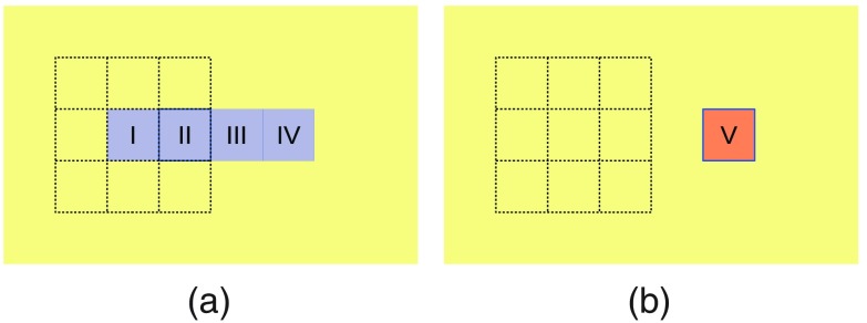
Note that the local overlap-based metrics may not be computable in some of the boundary neighborhoods. For instance, if we consider $x$ on $\partial G$ and $|M(N_x)|=0$, then $\mathrm{Prec}(N_x)$ is unknown (zero divided by zero). Because such cases indicate a mismatch of the boundaries, we want to decrease their score and, hence, we replace such unknowns with zeroes in the above definitions. A simplified example is presented in Fig. 4. In this example, the ground truth consists of four pixels (I to IV) and the machine segmentation consists of single pixel V, which overlaps with pixel IV of the ground truth. The precision metric is undefined in the local Moore neighborhoods of pixels I and II. In the neighborhoods of pixels III and IV, the precision score is 1 [both the local intersection $G(N_{IV})\cap M(N_{IV})$ and the local machine segmentation $M(N_{IV})$ count exactly one pixel, IV]. The neighborhood of pixel V is the same as the neighborhood of pixel IV, hence that neighborhood has a precision score of 1. If we were to exclude the neighborhoods with undefined precision from the SBP definition, this machine segmentation would get a best attainable SBP score of $\frac{3\times 1}{3}=1$. When we replace the unknowns with zeroes, the SBP score of this example becomes $\frac{2\times 0+3\times 1}{5}=0.6$, a more realistic figure.

Fig. 4.

A simplified segmentation case with undefined local precision in some of the boundary neighborhoods. (a) Ground truth pixels I to IV; (b) machine segmentation pixel V. The highlighted Moore neighborhood of pixel I contains no machine segmentation pixels, hence the precision metric is undefined there.

Table 1 lists the newly defined metrics in the family; an experimental comparison of these new metrics is given in Sec. 5.

Table 1.

Proposed boundary-overlap-based similarity metrics: directional and symmetric variants.

Boundary Dice metrics	Boundary Jaccard metrics
${\mathrm{DBD}}_G=\frac{\sum _{x\in \partial G}\mathrm{DSC}(N_x)}{|\partial G|}$	${\mathrm{DBJ}}_G=\frac{\sum _{x\in \partial G}\mathrm{JSC}(N_x)}{|\partial G|}$
${\mathrm{DBD}}_M=\frac{\sum _{y\in \partial M}\mathrm{DSC}(N_y)}{|\partial M|}$	${\mathrm{DBJ}}_M=\frac{\sum _{y\in \partial M}\mathrm{JSC}(N_y)}{|\partial M|}$
$\mathrm{SBD}=\frac{\sum _{x\in \partial G}\mathrm{DSC}(N_x)+\sum _{y\in \partial M}\mathrm{DSC}(N_y)}{|\partial G|+|\partial M|}$	$\mathrm{SBJ}=\frac{\sum _{x\in \partial G}\mathrm{JSC}(N_x)+\sum _{y\in \partial M}\mathrm{JSC}(N_y)}{|\partial G|+|\partial M|}$
Boundary TPVF metrics	Boundary TNVF metrics
${\mathrm{DBTP}}_G=\frac{\sum _{x\in \partial G}\mathrm{TPVF}(N_x)}{|\partial G|}$	${\mathrm{DBTN}}_G=\frac{\sum _{x\in \partial G}\mathrm{TNVF}(N_x)}{|\partial G|}$
${\mathrm{DBTP}}_M=\frac{\sum _{y\in \partial M}\mathrm{TPVF}(N_y)}{|\partial M|}$	${\mathrm{DBTN}}_M=\frac{\sum _{y\in \partial M}\mathrm{TNVF}(N_y)}{|\partial M|}$
$\mathrm{SBTP}=\frac{\sum _{x\in \partial G}\mathrm{TPVF}(N_x)+\sum _{y\in \partial M}\mathrm{TPVF}(N_y)}{|\partial G|+|\partial M|}$	$\mathrm{SBTN}=\frac{\sum _{x\in \partial G}\mathrm{TNVF}(N_x)+\sum _{y\in \partial M}\mathrm{TNVF}(N_y)}{|\partial G|+|\partial M|}$
Boundary Prec metrics
${\mathrm{DBP}}_G=\frac{\sum _{x\in \partial G}\mathrm{Prec}(N_x)}{|\partial G|}$
${\mathrm{DBP}}_M=\frac{\sum _{y\in \partial M}\mathrm{Prec}(N_y)}{|\partial M|}$
$\mathrm{SBP}=\frac{\sum _{x\in \partial G}\mathrm{Prec}(N_x)+\sum _{y\in \partial M}\mathrm{Prec}(N_y)}{|\partial G|+|\partial M|}$

3.2. Parameterization

Each boundary overlap metric can be parameterized by the neighborhood radius; and thereby, increase or decrease the visibility of local overlap. In our current experiments, we consider cube-shaped Moore neighborhoods of radius 1 (i.e., 9- and 27-neighborhoods in 2-D and 3-D, respectively), all the way up to radius 5, and we compare experimentally the performance of SBD for each radius. This systematic study follows in Sec. 4.3.2.

3.3. Implementation and Complexity

Algorithm 1 presents how SBD can be implemented for 2-D images. The Neighb procedure returns the set of positions in the Moore neighborhood of point $p$ with radius. The Boundary procedure constructs and returns the set of points on the boundary of mask, a binary representation of a region. The Subarray procedure constructs a submask with radius of the given mask at position pos. DSC and SBD are the procedures that calculate the corresponding metrics.

Algorithm 1.

The calculation of SBD in 2-D.

1: procedure SBD (gt, ms, radius) ▹ The SBD of the gt and ms binary masks

2: $sum\leftarrow 0$

3: $number\leftarrow 0$

4: for all$pos\in$Boundary (gt, radius) $+$Boundary (ms, radius) do ▹ position may be considered twice

5:  gtsub ← Subarray (gt, pos, radius)

6:  mssub ← Subarray (ms, pos, radius)

7:  sum ← sum + DSC (gtsub, mssub)

8:  $number\leftarrow number+1$

9: end for

10:return$sum÷number$

11: end procedure

12: procedureBoundary (mask, radius) ▹ The Boundary of the mask with given radius

13: for all$p\in positions$do ▹ positions is the set of positions in mask

14:  if$mask[p]$and$\exists q\in$Neighb ($p,radius$), $\neg mask[q]$then

15:   yield$p$ ▹ include $p$ in the Boundary set

16:  end if

17: end for

18: end procedure

In terms of complexity, boundary overlap metrics allow for straightforward implementation which is linear in region size. From this perspective, they are more similar to overlap metrics and outperform boundary distance metrics, which have to consider all the pairs of points from the two boundaries (although nearly linear implementations exist for these³²).

4. Experimental Results

The existing metrics disagree greatly: some metrics are sensitive to specific types of errors while other metrics are not, and vice versa for other images. Depending on the clinical application, different aspects of the evaluation can take priority: sometimes errors in the shape are more important (e.g., cancerous tissue), sometimes the precise location is crucial (e.g., in radiotherapy), other times it is the overall volume that matters more (e.g., in volume evaluation of lung cancer). In an ideal world, the evaluation of any segmentation procedures would be carried out with feature-specific metrics. In practice, existing metrics have often been “inherited” from past research and are being used without particular attention to the type of error that they reveal. For example, the DSC has become a “classic,” even if good performance measured the Dice way is not necessarily relevant to the application.³³

4.1. Synthetic Data

Before we look at medical scan data (in Sec. 4.2), we first investigate SBD using a set of 2-D synthetic images carefully constructed so as to demonstrate instances where the existing metrics fail. The collection in Figs. 5 and 6 contains simple geometric shapes (rectangle, disc, ellipse, and star) and fractals, in order to enable us to reason about and visualize the behavior of both old and new comparison metrics. For each shape, there are images (left column) to serve as ground truth and a sequence of synthetic images (right columns) to simulate segmentation results. These shapes are constructed to simulate departure from the ground truth in size, location, orientation, or combinations thereof. Another potential departure from the ground truth can be in voxel or group-of-voxels errors; these are simulated by “salt-and-pepper” pixels in the synthetic segmentations. The salt-and-pepper pixels are obtained by flipping pixels in the synthetic ground truth image with some probability. Disc, ellipse, and star images 9 and 10 are constructed by flipping pixels inside the white region with 20% and 5% probabilities, respectively. Corresponding images 11 and 12 are achieved by flipping all image pixels with 5% and 0.1% probabilities.

Fig. 5.

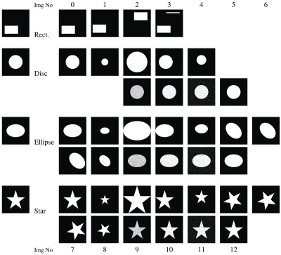
Synthetic dataset: ground truth images (left column) along with images for segmented regions incorporating size, location, shape, simulated salt-and-pepper errors in the segmentation, or combinations. The text refers to these images with a combination of one of the letters “r,” “d,” “e,” or “s,” and a number: r0 corresponds to the first—and ground truth—rectangle image; d12 is the last disc image, etc.

Fig. 6.

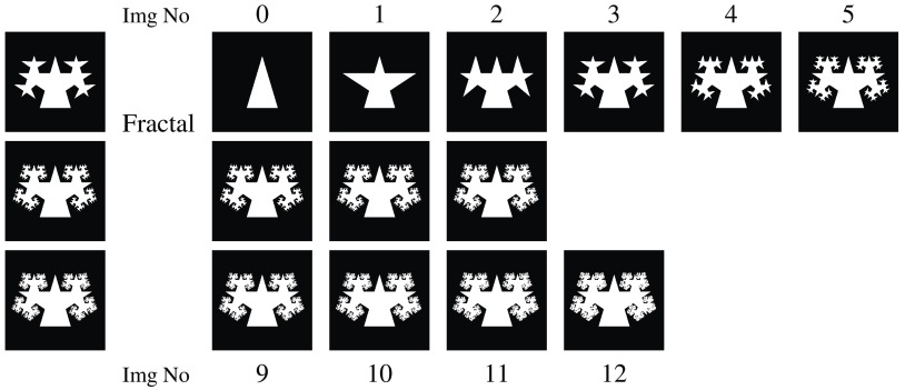
Sequence of synthetic fractal images with new isosceles triangles added at each recursive step (0 to 12). The three images at steps 3, 6, and 9—used as ground truth—are also presented in the left column. The text refers to these images with a combination of the letter “f” and a number: f6 is the image at recursive step 6; f12 is the image at recursive step 12, i.e., the last image.

We proceed to compare the white or near-white regions in the right-hand columns (representing potential segmentation results) against the white region in the left-hand column (representing ground truth).

4.1.1. Simple geometric shapes

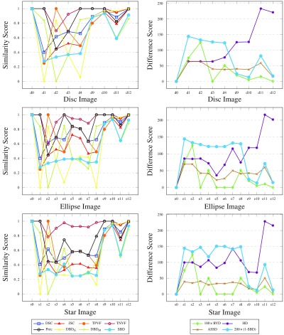
Our experiments in Figs. 7 and 8 compare the segmented images against the ground truth using the existing metrics and some of our boundary overlap metrics. While most conventional metrics are unable to differentiate clearly between images in a given sequence, SBD assigns them each a different score. Note that some of the difference metrics have been scaled in the graphs to be brought into similar value ranges. Such differences are the result of varying metric units.

Fig. 7.

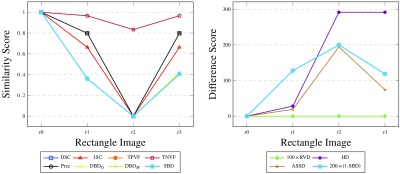
Results for synthetic rectangle images, comparing the segmented images against the ground truth, with all the considered metrics. Note that DSC, TPVF, and Prec scores are identical for all four images and their plots are not easily traced (similarity graph on the left). Likewise, ${\mathrm{DBD}}_G$ and ${\mathrm{DBD}}_M$ plots are almost identical with SBD.

Fig. 8.

Results for synthetic disc, ellipse, and star images, comparing the segmented images against the ground truths, with all the considered metrics. Note that some overlap-based (boundary-distance-based) scores are equal in the left graphs (right graphs) for a few images and their plots are not easily traced.

Our results show that SBD generally penalizes segmentation errors more than the other metrics, resulting in a wider (and hence easier to use) range of scores. The score assigned to the synthetic images designed with segmentation errors by most existing metrics is frequently the best attainable one. A few examples of such unfair scoring in Fig. 8 include Prec and TNVF scores for images e8 to e10, RVD scores for images s5 to s7, TPVF scores for d2 and e2, etc. By contrast, SBD never assigns the best attainable score to an image with an obvious segmentation fault. For images with simulated salt-and-pepper errors in the segmentation (disc, ellipse, and star images 9 to 12), where other metrics mostly disagree, SBD averages the overoptimistic scores of overlap-based metrics and the overpessimistic scores of boundary-distance-based metrics. In other words, SBD penalizes the random false negatives inside and false positives outside of the expected shapes more than the overlap metrics and less than the boundary distance metrics do.

SBD also assigns a low score to all images featuring some mismatch against the ground truth, thus showing better sensitivity to a larger span of error types. The directional variants of boundary Dice (${\mathrm{DBD}}_G$ and ${\mathrm{DBD}}_M$) show interestingly contradictory results for images where other metrics evidently disagree; these contradictions are neutralized in the symmetric variant (SBD).

4.1.2. Examples for discussion

We revisit the examples from Sec. 2.4 in order to analyze the performance of existing metrics and SBD. Note that the synthetic images for rectangle shape (r0 as ground truth, r1 to r3 as segmented, see Fig. 5) correspond to the discussed cases in Figs. 2(a)–2(c); and Figs. 2(d) and 2(e) match disc images d1 and d2 (d0 is the ground truth). Evidently, such extreme segmentation faults are rare in real world situations. We chose to use these so as to simplify the demonstration: we care less about the quality of the segmentation and are only interested in how the metrics react to such segmentation faults.

As expected, the RVD score is zero throughout the rectangle examples (see Fig. 7) since the sizes of the ground truth and the segmented regions are the same. The overlap-based metrics—DSC, JSC, TPVF, TNVF, Prec—give equal scores to the r1 and r3 images ignoring the different location errors in these images. HD fails to differentiate between images r2 and r3. The only two metrics that assign different scores to all four images are ASSD and SBD, although they disagree on the ranking of the r1 and r3 images: while ASSD claims r1 to be better, SBD prefers r3 since there is an absolute match of a segment of the boundary in this image with the ground truth.

Let us imagine that we want to rank the three rectangle segmentations (r1 to r3) with respect to the ground truth r0. DSC ranks r1 and r3 as a shared first with a score of 80%; r2 is third with 0% (see Fig. 7 left). HD ranks r1 first with a distance score of 28 units; r2 and r3 are second with an extremely high distance score of 292 units (see Fig. 7 right) and can be considered as failed segmentation results. Should r3 be considered a relatively good segmentation or should it be considered as a total failure? Evidently, r2, also Fig. 2(b), is a worse result than r3, also Fig. 2(c), and this should be reflected in the evaluation scores and the segmentation ranking. It can be argued that for specific tasks, where correct location of boundaries is a priority, r3 can be considered a better segmentation than r1. This is because most false positives in r3 can be removed automatically by an algorithm which deletes the disconnected rectangle at the top of Fig. 2(c). However, we acknowledge that the expected ranking of the images can be arguable and task-dependent; hence, the choice of evaluation metric should also be task-dependent.

As discussed in Sec. 2.4 and illustrated in Figs. 2(d) and 2(e), the boundary-distance-based metrics (HD, ASSD) score images d1 and d2 identically. Some of the overlap-based metrics assign the best attainable scores to these images: TNVF, Prec to image d1; TPVF to d2. Image d1 is preferred to image d2 by TNVF, Prec, and RVD; while d2 is considered better by DSC, JSC, TPVF, and SBD. It is worth noting that the directional variants of boundary Dice (${\mathrm{DBD}}_G$ and ${\mathrm{DBD}}_M$) successfully highlight the total mismatch of the ground truth and segmented boundaries with ${\mathrm{DBD}}_G=0$ for d1 and ${\mathrm{DBD}}_M=0$ for d2. SBD gives the two images scores of 0.278 and 0.335, which are sufficiently low to indicate segmentation errors in both cases, and are nonequal to point out that the errors are different.

Images d9–d12, e9–e12, and s9–s12 with simulated salt-and-pepper errors have been constructed to analyze the sensitivity of the considered metrics to random segmentation errors. The overlap-based metrics class d12, e12, and s12 as near-perfect segmentation results and rank them higher than d1 to d4 and d9 to d11, e1 to e11, s1 to s11, respectively. However, boundary-distance-based metrics such as HD rank images d12, e12, and s12 as second worst in their corresponding image sequences. The high but not the best attainable similarity scores that SBD assigns to these images indicate three properties: first, the random errors are reflected in the scores; second, the errors in these images affect the segmentation quality less than the errors in images such as e1 to e8, s1 to s8; third, such random errors are easier to eliminate in segmentation postprocessing.

4.1.3. Fractals

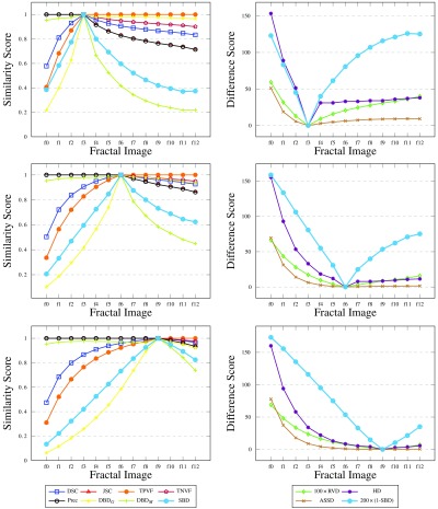
Additional to the simple shapes, the synthetic data contain a sequence of fractals (Fig. 6). These help reveal how the metrics react to boundary errors, where the boundary consists of increasingly intricate detail. The initial region is an isosceles triangle (image f0). At each step of the recursion, new triangles with the same ratio of side lengths $(4:7)$ are added on the equal sides of each triangle. The images from steps 3, 6, and 9 of the recursion are assigned as ground truth in turn, producing the results reported in Fig. 9.

Fig. 9.

Results for synthetic fractals. Fractals at steps 3, 6, and 9 of the recursion considered as ground truth, respectively.

The graphs illustrate interesting patterns. Images f0 to f2 (f0 to f5, f0 to f8) are undersegmented, and images f4 to f12 (f7 to f12, f10 to f12) are oversegmented. Note, on the one hand, that the conventional metrics DSC (and JSC), TPVF, HD, and ASSD show more variability for the undersegmented images—they fail to differentiate properly the oversegmented images. On the other hand, TNVF and Prec are insensitive to undersegmentation errors. The directional variants of the new metric show similar behavior to the first and the second group of metrics, respectively. RVD performs relatively better but still fails to capture differences at the level of local neighborhoods on the region boundary.

By contrast, SBD easily identifies the under- and oversegmentation errors, and reflects those in its scoring. It shows high sensitivity to even small differences between the boundaries of the ground truth and segmented images, and uses a wide scoring range to illustrate those differences. For DSC, HD, or ASSD, the differences in score for images f0 to f2 (f0 to f5, f0 to f8) are significantly higher than for images f4 to f12 (f7 to f12, f10 to f12). Unlike the existing metrics, SBD uses a similar range of values on both sides of the ground truth. These examples showcase how well SBD outperforms all the other metrics, especially for segmentation errors near the boundary of the intended region.

4.2. Real Scan Data

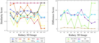
We ran a segmentation algorithm⁸ on nine different CT scan 3-D images, between 1 and 38 slices each. We automatically labeled 13 kidneys (left or right), for which we also manually produced ground truth masks. The results of validating the segmented 3-D images against the ground truths are presented in Fig. 10.

Fig. 10.

Results for medical kidney scans, i.e., 3-D regions in 3-D images. Results for 11 kidneys (left or right) from nine 3-D medical CT scans, between 1 and 38 slices each. Note that some overlap-based scores are identical in the left graph for a few images and their plots are not easily traced.

Since the machine segmentation results are produced by a single automated algorithm, errors of a similar nature are expected in all cases. The small ranges of score values produced by the various metrics illustrate this. TNVF values are all above 99%, due to the kidney occupying only a small portion of the 3-D image voxels. TPVF and Prec scores are complementary on most images: one of these metrics is only sensitive to undersegmentation and the other one—to oversegmentation. As was the case with 2-D synthetic images, SBD tends to penalize errors more harshly, producing smaller similarity scores (and hence, higher difference scores) than most existing metrics. In this experiment, its value range agrees better with DSC, JSC, and HD.

When there is great disagreement between classes of metrics or between metrics inside a class, such as in k10 and k11, SBD acknowledges the errors without being overly sensitive to the error. These two kidney segmentations are ranked higher than k1 to k9 by Prec, HD, and ASSD. At the same time, DSC, JSC, TPVF, and RVD penalize these segmentations ranking them lowest. SBD is the only metric that does not yield extreme scores for these two cases; its directional variants (${\mathrm{DBD}}_G$ and ${\mathrm{DBD}}_M$) do, as do the two groups of conventional metrics.

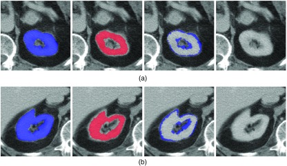
The great disagreement of the existing metrics for these two particular kidneys is explained by the variation in the number of slices in the images considered. Images k10 and k11 consist of only a single CT slice. The number of CT slices for k1 to k9 is at least 5, where k1 is the biggest image with 38 slices. We present the ground truth and the automated segmentation of k10 and k11 in Fig. 11. For comparison, we report a few slices from k1 in Fig. 12. This is a typical example where, although DSC is high (93%), at the same time the images show a poor segmentation around the boundary: 9(b) leaks and 9(c) presents salt-and-pepper errors (of the sort we simulated in the synthetic data). A further study of the effect of image size on the metric scores is presented in Sec. 4.3.3.

Fig. 11.

The labeled regions are: blue ground truth GT (first column), red machine segmentation⁸ MS (second), GT\MS (third), and MS\GT (last). These are shown for (a) k10 and (b) k11. In each case, the automated segmentation contains slightly fewer pixels than the ground truth (i.e., is slightly undersegmented).

Fig. 12.

The labeled regions are: blue ground truth GT (first column), red machine segmentation⁸ MS (second), GT\MS (third), and MS\GT (last). These are shown for three different slices (a)–(c) of k1. On close inspection, these slices present examples of undersegmentation, oversegmentation, and also random errors, each of the order of a few pixels. The random errors are similar to our simulated salt-and-pepper and are visible in the second and third columns in (c).

In order to preserve the level of detail in the graphs, Fig. 10 does not include data points for two kidney scans with pathological cases where the ground truth disagreed strongly with the machine segmentation. For these images, the machine segmented 3-D region was more than 3.5 times larger than the ground truth (because the human operator decided not to include any necrotic tissue in the ground truth). SBD scored these kidney segmentations around 0.33 and 0.38, sharing the sensitivity of other metrics: DSC of 0.28 and 0.34, and HD of 97 and 85 mm. RVD flags this stark difference and should always be applied first, as a sanity check.

4.3. Further Tests

4.3.1. Ranking tests

We set up a small experiment in order to understand the correlation between segmentation rankings produced with evaluation metrics and end user expectations. For that, we asked four researchers in image segmentation to rate the synthetic fractal images (Fig. 6) against the ground truth image f6. They were offered a discrete scoring range of 0 to 10, where 0 indicates segmentation failure and 10 indicates that the segmented region matches the ground truth perfectly. There was a mutual agreement that this scoring range was adequate to rank the images (f0 to f12) unambiguously.

The comparison of the averaged human ranking (mapped from 0 to 10 onto [0,1]) of the fractal images and the considered metrics, including SBD, is reported in Fig. 13. We exclude those metrics that produce the best attainable scores on one or the other side of the ground truth—TPVF, TNVF, and Prec (see Fig. 9). Difference metrics have been scaled and converted into corresponding similarity metrics to fit the scoring range between 0 and 1. As the graphs show, the human ranking correlates best with SBD with a single ranking disagreement at f4. In addition, their maximum absolute difference in score per image stands at less than 9.3%. For comparison, corresponding differences between the human ranking and DSC or $1-\mathrm{RVD}$ stand at more than 44.6% or 29.5%. These are encouraging initial results for possible future study of ranking properties of evaluation metrics versus human perception of segmentation results.

Fig. 13.

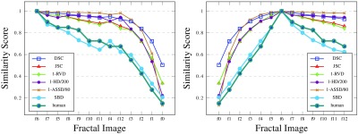
The ranking of the fractal images with different metrics with the ground truth set at f6. The images are sorted in the order of human ranking in the first graph; the second graph preserves the order of fractal recursion.

4.3.2. Parameterization tests

In addition to comparing SBD to existing and commonly used metrics, we analyzed how the SBD performance changes based on its parameterization. Consistently changing the Moore neighborhood radius from 1 to 5 for the synthetic data, we reveal that SBD similarity scores gradually increase for larger radii (for most images). The growth is around 9% to 10% between radius 1 and 5 in average, although for specific segmentation results it reaches 46% to 47%. Our overall conclusion here is that the simple neighborhood with radius 1 should be generally preferred (in the case of fixed resolution experiments). Increasing the size of neighborhood has only a minor effect on similarity score values and ranges but extends execution times.

The sample graphs in Fig. 14 depict how the SBD values vary with the change in Moore neighborhood radius from 1 to 5. The growth of the neighborhood size causes only a tiny rise in the similarity score for most images. For a few images this is slightly more noticeable, e.g., ellipse images e6 and e11 feature a score increase of 30% to 32%.

Fig. 14.

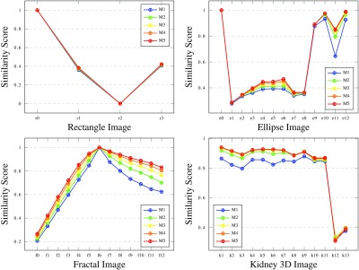
Comparison of SBD results for rectangle, ellipse, and fractal (ground truth at step 6) images and medical kidney 3-D images using Moore neighborhoods of radius 1 to 5. Note that some SBD scores with different neighborhood radii are equal or have very close values for a few images, and their plots are not easily traced.

When the neighborhood size increases, more internal points of the segmented regions end up labeled as boundary points. Those, in turn, introduce higher local similarity Dice scores; thus, for the new extended set of local scores, the average increases. Table 2 presents additional data for star images illustrating this trend. The lower bounds of value ranges and average scores (over 13 star images) form increasing sequences, from lower neighborhood sizes to larger ones. It is important to note that the average score rise is only from 0.509 to 0.552. This growth in scores for larger neighborhoods means (only slightly) decreased sensitivity to segmentation errors; therefore, we propose generally using simple neighborhoods of radius 1.

Table 2.

Value ranges and average values of SBD results over 13 star images using Moore neighborhoods of radii 1 to 5.

Moore radius	1	2	3	4	5
Value range	0.246 to 1	0.258 to 1	0.265 to 1	0.272 to 1	0.276 to 1
Average	0.509	0.534	0.543	0.548	0.552

Finally, we considered how the execution time increases for larger neighborhood radii. We implemented a Python SBD scoring script for a sequence of synthetic images against a single ground truth for a user-set neighborhood radius. The real execution time of the program ranged between 10.8 s and 3 min 7.4 s (12 s and 3 min 22.3 s) for the 13 fractal images, where image f3 (f6) was taken as ground truth. The lowest and highest running times in these ranges correspond to radii 1 and 10. In both cases, the execution times show monotonic growth with the increase of the radius between 1 and 10. This fact supports our preference for smaller neighborhoods.

4.3.3. Size and resolution tests

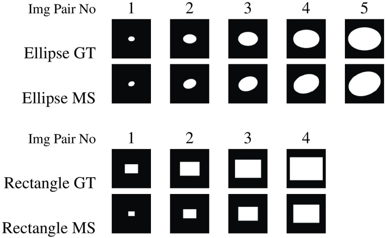
A further aspect of interest is the response of the metrics to variations in the size of segmented regions and in image resolution. Figure 15 lists the contents of a small synthetic dataset that was constructed to analyze the impact of region size and image resolution variations on metric scores. The corresponding evaluation results for region size variation are reported in Table 3. Most existing metrics for the five ellipse image pairs behave very differently from the same metrics for the four rectangle image pairs. An exception to this pattern is seen for TNVF and Prec. For the five ellipse image pairs, TNVF is absolutely insensitive to the errors in the image pairs with smaller regions (ellipse image pairs 1–2) and slightly more sensitive for the larger regions (ellipse image pairs 4–5). Prec is stably high for the five ellipse image pairs. The best attainable TNVF and Prec scores for the four rectangle image pairs are explained by their total insensitivity to undersegmentation.

Fig. 15.

A small collection of simulated machine segmentation (MS) and ground truth (GT) image pairs with monotonically increasing region size based on ellipse and rectangle shapes. The image resolution is set at $512\times 512$.

Table 3.

The impact of region size variation on metric scores using simulated segmentation images with ellipse and rectangle shapes.

	DSC	JSC	TPVF	TNVF	Prec	RVD	HD	ASSD	SBD
Ellipse pair
1	0.921	0.854	0.922	0.999	0.921	0.000	5.000	2.606	0.502
2	0.923	0.857	0.923	0.995	0.922	0.001	8.944	5.307	0.460
3	0.922	0.855	0.922	0.987	0.922	0.000	13.454	8.150	0.441
4	0.922	0.855	0.922	0.974	0.922	0.000	17.692	10.974	0.434
5	0.922	0.855	0.922	0.950	0.921	0.000	21.932	13.816	0.428
Rectangle pair
1	0.397	0.248	0.248	1.000	1.000	0.752	52.202	36.748	0.264
2	0.614	0.443	0.443	1.000	1.000	0.557	53.600	36.225	0.319
3	0.720	0.562	0.562	1.000	1.000	0.438	51.865	35.720	0.342
4	0.780	0.639	0.639	1.000	1.000	0.361	52.431	35.717	0.355

The other overlap-based metrics (DSC, JSC, and TPVF) and the size-based RVD metric maintain approximately the same value for all five ellipse image pairs. The boundary-distance-based metrics (HD, ASSD), on the other hand, gradually increase for these examples indicating higher dissimilarity for the image pairs with larger region sizes. SBD is in agreement with the boundary-distance-based metrics for these examples, considering the match of the smaller regions in ellipse image pairs 1–2 to be better than the match of the larger regions in ellipse image pairs 4–5.

DSC, JSC, TPVF, and RVD show significant variation for the four rectangle examples: image pairs 1–2 get significantly lower similarity (higher difference) scores than image pairs 3–4. On the other hand, HD and ASSD values are relatively stable for the rectangle image pairs. SBD agrees with the former metrics, considering rectangle image pair 1 to be the worst, and rectangle image pair 4 the best out of the four cases.

The slow decrease in SBD scores for ellipse image pairs is explained by the local overlaps in the neighborhoods of boundary points shrinking as the regions get bigger and their boundaries diverge. In the case of the rectangles, the distance between the boundaries stays the same; hence, the local overlap scores do not change. It is the ratio of the boundary lengths that affects the weights of the local overlaps and leads to the small increase in SBD values for the rectangle image pairs. The monotonic change of the SBD scores in accordance with region size is inherent to its definition and reflects its hybrid nature between overlap metrics and boundary distance metrics.

In Table 4, we report how image resolution affects the scores of the metrics. DSC, JSC, TPVF, TNVF, Prec, and RVD maintain their values for all resolutions. In the case of HD and ASSD, the scores increase by a factor of 2 in parallel with image resolution because our calculation does not take into account physical dimensions of pixels. In a clinical setting, those dimensions would decrease by a factor of 2 when the resolution increases, thus keeping the metric scores to the original values.

Table 4.

The impact of image resolution variation on metric scores using simulated segmentation images with ellipse shape. A single pair of ellipse GT and MS images is considered at resolutions from $128\times 128$ to $2048\times 2048$.

Resolution	DSC	JSC	TPVF	TNVF	Prec	RVD	HD	ASSD	SBD
$128\times 128$	0.923	0.857	0.924	0.987	0.921	0.003	3.606	1.898	0.535
$256\times 256$	0.923	0.857	0.923	0.987	0.923	0.000	6.708	3.932	0.476
$512\times 512$	0.922	0.855	0.922	0.987	0.922	0.000	13.454	8.150	0.441
$1024\times 1024$	0.922	0.855	0.922	0.987	0.922	0.000	26.401	16.645	0.424
$2048\times 2048$	0.922	0.855	0.922	0.987	0.922	0.000	52.802	33.475	0.419

SBD scores go down slightly as image resolution increases, as reported in Table 4. Increasing image resolution is equivalent to decreasing neighborhood size for SBD, since it makes the region boundary thinner. Selecting larger SBD neighborhood radii for higher resolution images would keep SBD scores at the same level.

For general use, when experimental results for images of varying pixel resolution need to be compared, the neighborhood radius for SBD can be chosen based on the physical dimensions of pixels. For instance, the neighborhood radius can be set to 1 for 4 mm pixel images, set to 2 for 2 mm pixel images, and set to 4 for 1 mm pixel images. This will keep the SBD value range consistent for images of different resolutions.

5. Comparison of Boundary Overlap Methods

In Sec. 3.1, we defined a number of new boundary-overlap-based metrics. So far, in our experiments for comparison against conventional metrics we used only one of them—SBD. This was done in order to prove the concept without overburdening the discussion and the performance graphs. We now turn to analyze the performance of all the boundary overlap metrics in the family.

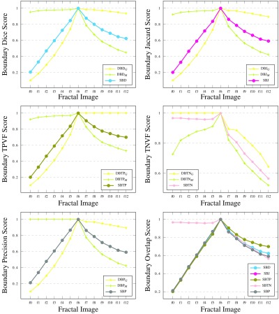
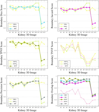
In Fig. 16, we report the comparison of all the new metrics on the fractal synthetic data with ground truth f6. Figure 17 shows the corresponding results for the real kidney data. From the results in the first set of graphs, the behavior of all the metrics is very similar except the boundary true negative fraction (both directional and symmetric). SBTN is insensitive to the undersegmented fractal steps f0 to f5, but on images f7 to f12 it performs relatively similar to the other metrics. The insensitivity is a consequence of the peculiar definition of this metric. Around ground truth boundary points, it gives the best attainable local neighborhood score if the machine segmentation is absent from that neighborhood: $\mathrm{TNVF}(N_x)=\frac{|N_x|-|M(N_x)\cup G(N_x)|}{|N_x|-|G(N_x)|}=1$ if $|M(N_x)|=0$.

Fig. 16.

Different boundary overlap metrics (their directional and symmetric variants) compared on the synthetic fractal images with ground truth f6. The first five graphs correspond to boundary Dice, Jaccard, TPVF, TNVF, and precision metrics. The sixth graph combines the symmetric variants of all five metrics.

Fig. 17.

Different boundary overlap metrics (their directional and symmetric variants) compared on the real kidney 3-D images. The first five graphs correspond to boundary Dice, Jaccard, TPVF, TNVF, and precision metrics. The sixth graph combines the symmetric variants of all five metrics.

Once again, in Fig. 17, the SBTN scores disagree with the rest, this time assigning much lower scores in each case. In cases where the machine segmentation boundary includes the ground truth (oversegmentation), this leads to the overall SBTN score being lower, thus penalizing such segmentations. $\mathrm{TNVF}(N_y)=\frac{|N_y|-|M(N_y)\cup G(N_y)|}{|N_y|-|G(N_y)|}=1-\frac{|M(N_y)|}{|N_y|}$ if $|G(N_y)|=0$ where $y\in \partial M$. When the machine segmentation boundary is included inside the ground truth (undersegmentation), the SBTN score is higher, due to an increase in the local TNVF. However, when the undersegmentation is substantial, i.e., a considered neighborhood is fully inside the ground truth, the local TNVF value is not defined. The latter is the case with our particular kidney segmentations; hence, the overall SBTN score is lower.

We explain the occasional disagreement of the SBD, SBJ results with SBTP and SBP (and between SBTP and SBP) by the directional complementary nature of the overlap-based TPVF and Prec metrics used in the local neighborhoods. Hence, on some of the examples, the insensitivity to the local errors causes higher scores with these metrics. For instance, kidney images k1, k2, k4, and k6 get high SBTP scores, while high SBP scores are recorded for images k5, k10, and k11.

Unsurprisingly, the metrics introduced in this paper inherit features from the corresponding overlap-based metrics. For instance, the value range of the new metrics is between 0 and 1 (similar to the overlap-based metrics), where 1 indicates a perfect match and 0 indicates a total mismatch. Or, SBD and SBJ are linked, with SBJ values always being slightly smaller than SBD. However, they do not always produce the same ranking patterns. In the case of SBTN, when a local neighborhood size is fixed, an important feature is that it be independent of the size of the whole image (unlike the original TNVF metric). This fact is reflected in the huge difference of the value ranges of TNVF (see Fig. 10, $\ge 0.997$) and SBTN (Fig. 17, 0.066 to 0.56).

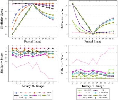
To summarize, Fig. 18 shows the comparison between the boundary overlap family and the existing metrics in a final set of graphs, using the synthetic fractal images with ground truth at f6 as well as the kidney 3-D scans. In order to preserve clarity, only symmetric variants of the new metrics are included in these graphs.

Fig. 18.

The performance of the conventional metrics against the proposed family of symmetric boundary overlap metrics on the examples of the synthetic fractal images with ground truth at f6 and the kidney 3-D images (excluding k12–k13).

6. Conclusions and Future Work

Our results demonstrate how, in contrast to existing metrics, SBD reacts to a wider range of error types. It penalizes errors more, producing a wider spread of similarity scores (lower for more errors). SBD does not incur score inflation, especially in cases where existing metrics disagree (one metric gives a high score and another gives a low one to the same segmentation result). The fractal experiments demonstrate that SBD is fit to evaluate segmentation results which are prone to error in the neighborhood of the region boundaries. Other members of the boundary overlap family have similar properties to SBD.

In the future, we will consider more segmentation rankings produced with other evaluation metrics; we will check whether SBD rankings correlate better than other metrics with human-produced rankings. An additional aspect of interest is to estimate how accurate a boundary overlap metric can be if not every point on the region boundaries is taken into account. For certain boundary shapes, this may be an option in order to improve execution time. Initial results for other metrics from our family suggest that these can also be used in segmentation evaluation. A caveat is that they inherit some of the limitations of the corresponding overlap-based metrics applied in the small neighborhoods. More experiments will follow with wider ranges of segmentation results, as well as further analysis of the strengths and weaknesses of this new family of metrics in comparison to metrics recently proposed in the literature.

In order for our family of metrics to be adopted into general use, it will be necessary to prove its effectiveness by conducting systematic studies of large publicly available medical datasets. Meanwhile, we propose SBD as the best and easiest to use out of the 15 metrics in the family because it is easy to implement, quick to run, and fulfills all the listed criteria for a good metric.

Biographies

Varduhi Yeghiazaryan is a doctoral student at the Department of Computer Science, University of Oxford. She received her BSc degree in applied mathematics and informatics from Russian-Armenian (Slavonic) University in 2012, and her MSc degree in computer science from the University of Oxford in 2013. She is a member of SPIE.

Irina Voiculescu is a senior lecturer at Oxford University Department of Computer Science. She received her PhD from the University of Bath, United Kingdom, for research in constructive solid geometry. Apart from her main interest in medical imaging (MRI and CT scan analysis), she has also been conducting research in areas such as molecular modeling (protein docking) and polynomial root finding (interval arithmetic).

Disclosures

The authors have no financial or any other conflicts of interest to declare.

References

- 1.Zhang Y. J., “Image segmentation evaluation in this century,” in Encyclopedia of Information Science and Technology, pp. 1812–1817, Tsinghua University, Beijing, China: (2009). [Google Scholar]
- 2.Udupa J. K., et al. , “A framework for evaluating image segmentation algorithms,” Comput. Med. Imaging Graphics 30(2), 75–87 (2006).https://doi.org/10.1016/j.compmedimag.2005.12.001 [DOI] [PubMed] [Google Scholar]
- 3.Cárdenes R., de Luis-García R., Bach-Cuadra M., “A multidimensional segmentation evaluation for medical image data,” Comput. Methods Programs Biomed. 96(2), 108–124 (2009).https://doi.org/10.1016/j.cmpb.2009.04.009 [DOI] [PubMed] [Google Scholar]
- 4.Zhang Y. J., “A survey on evaluation methods for image segmentation,” Pattern Recognit. 29(8), 1335–1346 (1996).https://doi.org/10.1016/0031-3203(95)00169-7 [Google Scholar]
- 5.Heimann T., et al. , “Comparison and evaluation of methods for liver segmentation from CT datasets,” IEEE Trans. Med. Imaging 28, 1251–1265 (2009).https://doi.org/10.1109/TMI.2009.2013851 [DOI] [PubMed] [Google Scholar]
- 6.Menze B. H., et al. , “The multimodal brain tumor image segmentation benchmark (BRATS),” IEEE Trans. Med. Imaging 34(10), 1993–2024 (2015).https://doi.org/10.1109/TMI.2014.2377694 [DOI] [PMC free article] [PubMed] [Google Scholar]
- 7.Maier O., Menze B., Reyes M., “ISLES challenge 2015,” www.isles-challenge.org/ISLES2015/ (27 January 2018).
- 8.Yeghiazaryan V., Voiculescu I. D., “Automated 3D renal segmentation based on image partitioning,” Proc. SPIE 9784, 97842E (2016).https://doi.org/10.1117/12.2216514 [Google Scholar]
- 9.Yeghiazaryan V., Voiculescu I., “An overview of current evaluation methods used in medical image segmentation,” Technical Report CS-RR-15-08, Department of Computer Science, University of Oxford, Oxford, United Kingdom: (2015). [Google Scholar]
- 10.Konukoglu E., et al. , “WESD–weighted spectral distance for measuring shape dissimilarity,” IEEE Trans. Pattern Anal. Mach. Intell. 35(9), 2284–2297 (2013).https://doi.org/10.1109/TPAMI.2012.275 [DOI] [PMC free article] [PubMed] [Google Scholar]
- 11.Dice L. R., “Measures of the amount of ecologic association between species,” Ecology 26(3), 297–302 (1945).https://doi.org/10.2307/1932409 [Google Scholar]
- 12.Linguraru M. G., et al. , “Statistical 4D graphs for multi-organ abdominal segmentation from multiphase CT,” Med. Image Anal. 16(4), 904–914 (2012).https://doi.org/10.1016/j.media.2012.02.001 [DOI] [PMC free article] [PubMed] [Google Scholar]
- 13.Wolz R., et al. , “Multi-organ abdominal CT segmentation using hierarchically weighted subject-specific atlases,” Lect. Notes Comput. Sci. 7510, 10–17 (2012).https://doi.org/10.1007/978-3-642-33415-3 [DOI] [PubMed] [Google Scholar]
- 14.Linguraru M. G., et al. , “Renal tumor quantification and classification in contrast-enhanced abdominal CT,” Pattern Recognit. 42(6), 1149–1161 (2009).https://doi.org/10.1016/j.patcog.2008.09.018 [DOI] [PMC free article] [PubMed] [Google Scholar]
- 15.Schenk A., Prause G., Peitgen H.-O., “Efficient semiautomatic segmentation of 3D objects in medical images,” Lect. Notes Comput. Sci. 1935, 186–195 (2000).https://doi.org/10.1007/b12345 [Google Scholar]
- 16.Lamecker H., Lange T., Seebass M., “Segmentation of the liver using a 3D statistical shape model,” Technical Report 4–9, ZIB, Berlin: (2004). [Google Scholar]
- 17.Campadelli P., Casiraghi E., Esposito A., “Liver segmentation from computed tomography scans: a survey and a new algorithm,” Artif. Intell. Med. 45(2–3), 185–196 (2009).https://doi.org/10.1016/j.artmed.2008.07.020 [DOI] [PubMed] [Google Scholar]
- 18.Liu Y., et al. , “An effective approach of lesion segmentation within the breast ultrasound image based on the cellular automata principle,” J. Digital Imaging 25(5), 580–590 (2012).https://doi.org/10.1007/s10278-011-9450-6 [DOI] [PMC free article] [PubMed] [Google Scholar]
- 19.Ruskó L., Bekes G., Fidrich M., “Automatic segmentation of the liver from multi- and single-phase contrast-enhanced CT images,” Med. Image Anal. 13(6), 871–882 (2009).https://doi.org/10.1016/j.media.2009.07.009 [DOI] [PubMed] [Google Scholar]
- 20.Chen X., et al. , “Medical image segmentation by combining graph cuts and oriented active appearance models,” IEEE Trans. Image Process. 21(4), 2035–2046 (2012).https://doi.org/10.1109/TIP.2012.2186306 [DOI] [PMC free article] [PubMed] [Google Scholar]
- 21.Grau V., et al. , “Improved watershed transform for medical image segmentation using prior information,” IEEE Trans. Med. Imaging 23, 447–458 (2004).https://doi.org/10.1109/TMI.2004.824224 [DOI] [PubMed] [Google Scholar]
- 22.Gan H.-S., et al. , “Interactive medical image segmentation with seed precomputation system: data from the osteoarthritis initiative,” in IEEE Conf. on Biomedical Engineering and Sciences (IECBES), pp. 315–318, IEEE; (2014).https://doi.org/10.1109/IECBES.2014.7047510 [Google Scholar]
- 23.Bağci U., Chen X., Udupa J. K., “Hierarchical scale-based multiobject recognition of 3-D anatomical structures,” IEEE Trans. Med. Imaging 31(3), 777–789 (2012).https://doi.org/10.1109/TMI.2011.2180920 [DOI] [PubMed] [Google Scholar]
- 24.Chen X., et al. , “3D automatic anatomy segmentation based on graph cut-oriented active appearance models,” in 17th IEEE Int. Conf. on Image Processing (ICIP), pp. 3653–3656 (2010).https://doi.org/10.1109/ICIP.2010.5652101 [Google Scholar]
- 25.Chen X., Bagci U., “3D automatic anatomy segmentation based on iterative graph-cut-ASM,” Med. Phys. 38, 4610–4622 (2011).https://doi.org/10.1118/1.3602070 [DOI] [PMC free article] [PubMed] [Google Scholar]
- 26.Campadelli P., Casiraghi E., Pratissoli S., “A segmentation framework for abdominal organs from CT scans,” Artif. Intell. Med. 50(1), 3–11 (2010).https://doi.org/10.1016/j.artmed.2010.04.010 [DOI] [PubMed] [Google Scholar]
- 27.Lim S.-J., Jeong Y.-Y., Ho Y.-S., “Automatic liver segmentation for volume measurement in CT images,” J. Visual Commun. Image Representation 17(4), 860–875 (2006).https://doi.org/10.1016/j.jvcir.2005.07.001 [Google Scholar]
- 28.Kauffmann C., Piché N., “Seeded ND medical image segmentation by cellular automaton on GPU,” Int. J. CARS 5(3), 251–262 (2010).https://doi.org/10.1007/s11548-009-0392-0 [DOI] [PubMed] [Google Scholar]
- 29.Gerig G., Jomier M., Chakos M., “Valmet: a new validation tool for assessing and improving 3D object segmentation,” Lect. Notes Comput. Sci. 2208, 516–523 (2001).https://doi.org/10.1007/3-540-45468-3 [Google Scholar]
- 30.Chen Y., et al. , “The domain knowledge based graph-cut model for liver CT segmentation,” Biomed. Signal Process. Control 7(6), 591–598 (2012).https://doi.org/10.1016/j.bspc.2012.04.005 [Google Scholar]
- 31.Yokota F., et al. , “Automated CT segmentation of diseased hip using hierarchical and conditional statistical shape models,” Lect. Notes Comput. Sci. 8150, 190–197 (2013).https://doi.org/10.1007/978-3-642-40763-5 [DOI] [PubMed] [Google Scholar]
- 32.Taha A. A., Hanbury A., “Metrics for evaluating 3D medical image segmentation: analysis, selection, and tool,” BMC Med. Imaging 15(1), 1–28 (2015).https://doi.org/10.1186/s12880-015-0068-x [DOI] [PMC free article] [PubMed] [Google Scholar]
- 33.Cuingnet R., et al. , “Automatic detection and segmentation of kidneys in 3D CT images using random forests,” Lect. Notes Comput. Sci. 7512, 66–74 (2012).https://doi.org/10.1007/978-3-642-33454-2 [DOI] [PubMed] [Google Scholar]