A new method to visualize obesity prevalence in Seattle‐King County at the census block level

Summary

Objective

The aim of this study is to map obesity prevalence in Seattle King County at the census block level.

Methods

Data for 1,632 adult men and women came from the Seattle Obesity Study I. Demographic, socioeconomic and anthropometric data were collected via telephone survey. Home addresses were geocoded, and tax parcel residential property values were obtained from the King County tax assessor. Multiple logistic regression tested associations between house prices and obesity rates. House prices aggregated to census blocks and split into deciles were used to generate obesity heat maps.

Results

Deciles of property values for Seattle Obesity Study participants corresponded to county‐wide deciles. Low residential property values were associated with high obesity rates (odds ratio, OR: 0.36; 95% confidence interval, CI [0.25, 0.51] in tertile 3 vs. tertile 1), adjusting for age, gender, race, home ownership, education, and incomes. Heat maps of obesity by census block captured differences by geographic area.

Conclusion

Residential property values, an objective measure of individual and area socioeconomic status, are a useful tool for visualizing socioeconomic disparities in diet quality and health.

Introduction

Obesity in the United States affects some groups more than others, particularly those with lower socioeconomic status (SES) as measured by education and income 1, 2. Both individual‐level and area‐level SES are also strong determinants of place, with a person's opportunities and resources often driven by surrounding economic means. However, to date, obesity prevalence maps by state and territory, county or metropolitan area 3, 4, 5 may not adequately capture sharp, observable inequities in health, at the local level, which are influenced by SES 6, 7. One problem is that geo‐located data on health or body weight are rarely available at a sufficiently fine geographic scale.

The lack of geographic coverage in health data has typically been remedied through modelling. For example, county‐level maps of obesity prevalence, released by Centers for Disease Control and Prevention, imputed missing data using small area estimation and Bayesian multilevel modelling. Close to 90% of the obesity data were, in fact, modelled using age, sex, race and Hispanic origin as predictor variables 8. Similarly, the award‐winning maps of US obesity rates by neighbourhood, developed by RTI International used age, gender, race, Hispanic origin and education as the chief modelling variables 9.

Previous work in Seattle‐King County 1, 10 and in Paris, France 11, demonstrated that higher obesity prevalence was more directly linked to lower SES than to age, gender, race or Hispanic origin. Two socioeconomic variables stood out as powerful predictors of prevalent obesity: residential property values and individual‐level educational attainment. The advantage of residential property values at the tax parcel level is that they can be readily geo‐localized, providing an objective index of individual‐level and area‐level poverty or wealth 12, 13. The present hypothesis was that a superior visualization of obesity prevalence across neighbourhoods would be obtained using a single unifying predictor variable: residential property values at tax parcel level.

Methods

Participants and procedures

Analyses were based on 1,632 Seattle and King County, WA residents, age 18 or older, who were participants in the previously described Seattle Obesity Study 13, 14. Individual‐level demographic, socioeconomic and weight data were collected via telephone survey. Annual household incomes were defined as: lower (<$50,000/year), middle ($50,000 to <$100,000/year) and higher income (≥$100,000). Educational attainment was defined as: <12 years (‘high school or less’), 12 to <16 years (‘some college’), and ≥16 years (‘college graduates or higher’). Body mass index (BMI = kg/m²) was based on self‐reported height and weight. Obesity was defined as body mass index < 30.

Home addresses were geocoded using ArcGIS Desktop 10 15. Tax parcel property values, per dwelling unit, of respondent residences were obtained from County Tax Assessor 14 and grouped into tertiles, following published procedures 14. All study protocols were approved by the University of Washington Institutional Review Board.

Statistical Analyses

Multiple logistic regression models examined the association between residential property values, education and income and obesity prevalence. Model 1 adjusted for age, gender, race and home ownership. Model 2 added income and education to Model 1. Model 3 added education and house prices to Model 1. McFadden's pseudo unadjusted and adjusted R² values were computed to assess the predictive value among the three models. Much lower than the conventional R² values, McFadden's pseudo‐R² values in the 0.2–0.4 range indicate a good model fit. All analyses were conducted using Stata version 14 (StataCorp LP, College Station, TX, USA) 16.

Obesity heat maps

First, mean obesity prevalence was calculated for each property value decile based on the regression model. Second, tax parcel‐level residential property values were aggregated by census block for all households in Seattle King County and split by deciles. Third, mean obesity prevalence was assigned to each census block by decile of property values. Heat maps used ArcGIS version 10 (Environmental Systems Research Institute, Redlands, CA, USA) 15.

Results

Table 1 shows that 20.7% (338/1,632) of Seattle Obesity Study participants were obese. Higher obesity rates in the Seattle‐King County sample were associated with lower SES indicators but not gender or race/ethnicity.

Table 1.

Study sample characteristics, by obesity status, Seattle Obesity Study I, 2008–2009

	Total		Obese
	N	%	N	%
Overall	1632	100.0	338	100.0
Sex
Male	658	40.3	147	43.5
Female	974	59.7	191	56.5
Age
18 to 44	426	26.1	79	23.4
45 to 54	407	24.9	79	23.4
55 to 64	432	26.5	108	32.0
65 or older	367	22.5	72	21.3
Race and ethnicity
White, non‐Hispanic	1322	81.0	276	81.7
Others	310	19.0	62	18.3
Own or rent current residence
Own	1282	78.6	247	73.1
Rent	350	21.4	91	26.9
Education
High school graduate or less	287	17.6	80	23.7
Some college or technical school	427	26.2	99	29.3
College graduate or higher	918	56.3	159	47.0
Annual household income
<$50,000	650	39.8	171	50.6
$50,000 to $99,999	563	34.5	111	32.8
≥$100,000	419	25.7	56	16.6
Residential property values at tax parcel
Low ($0–$229,193)	544	33.3	156	46.2
Medium ($229,290–$329,000)	546	33.5	119	35.2
High ($330,000‐$3,069,000)	542	33.2	63	18.6

Table 2 (Model 1) shows the expected associations between lower SES and higher obesity prevalence, adjusting for age, gender, race/ethnicity and home ownership (P < 0.05). When individual‐level education and income were included (Model 2), the effect of education persisted at college level, whereas the effect of income was attenuated. When individual‐level education and property values were included (Model 3), the association was stronger for property values (odds ratio, OR: 0.36, 95% confidence interval, CI [0.25, 0.51] for tertile 3 as compared with tertile 1) than for education (OR: 0.70, 95% CI [0.50, 0.97] for >16 vs. <12 years). Model 3 had the highest adjusted McFadden's pseudo‐R² (0.025), indicating that residential property values and educations were the best predictor variables.

Table 2.

Multivariable logistic regression analyses to compare three SES measures — income, education and residential property values in relation to obesity status, Seattle Obesity Study I, 2008‐2009

	Model 1
	OR [95% CI]	AIC	P‐value	R2	Adj R2
Education
High school graduate or less	Ref	1655.04	0.001	0.014	0.006
Some college or technical school	0.8 [0.56, 1.12]
College graduate or higher	0.57 [0.42, 0.79]
Annual household income
<$50,000	Ref	1647.16	<0.0001	0.019	0.011
$50,000 to $99,999	0.7 [0.52, 0.94]
≥$100,000	0.44 [0.30, 0.63]
Residential property values at tax parcel
Low ($0–$229,193)	Ref	1624.46	<0.0001	0.033	0.024
Medium ($229,290–$329,000)	0.72 [0.53, 0.97]
High ($330,000–$3,069,000)	0.33 [0.24, 0.47]
	Model 2
	OR [95% CI]	AIC	P‐value	R2	Adj R2
Education
High school graduate or less	Ref	1645.39	<0.0001	0.023	0.012
Some college or technical school	0.82 [0.58, 1.16]
College graduate or higher	0.67 [0.48, 0.93]
Annual household income
<$50,000	Ref
$50,000 to $99,999	0.74 [0.55, 1.00]
≥$100,000	0.49 [0.34, 0.72]
	Model 3
	OR [95% CI]	AIC	P‐value	R2	Adj R2
Education
High school graduate or less	Ref	1623.72	<0.0001	0.036	0.025
Some college or technical school	0.82 [0.58, 1.16]
College graduate or higher	0.70 [0.50, 0.97]
Residential property values at tax parcel
Low ($0–$229,193)	Ref
Medium ($229,290–$329,000)	0.74 [0.55, 1.00]
High ($330,000–$3,069,000)	0.36 [0.25, 0.51]

Model 1: Education, income, and residential property value were tested in separate models. Each model adjusted for age, gender, race and home ownership status. Model 2: Model 1 + added education and income in the same model. Model 3: Model 1 + added education and residential property values in the same model. Bold indicates statistical significance at the 0.05 level. AIC, akaike information criterion; OR, odds ratio; CI, confidence interval.

Figure 1 shows the spatial distribution of property values in Seattle King County. First, obesity was more prevalent in the lower‐income South Seattle compared with the more affluent North Seattle, consistent with data by Health Planning District collected by Public Health Seattle‐King County. Second, obesity prevalence was lower along waterfront residences and homes located closer to golf courses, parks and trails and higher closer to traffic and freeways.

Figure 1.

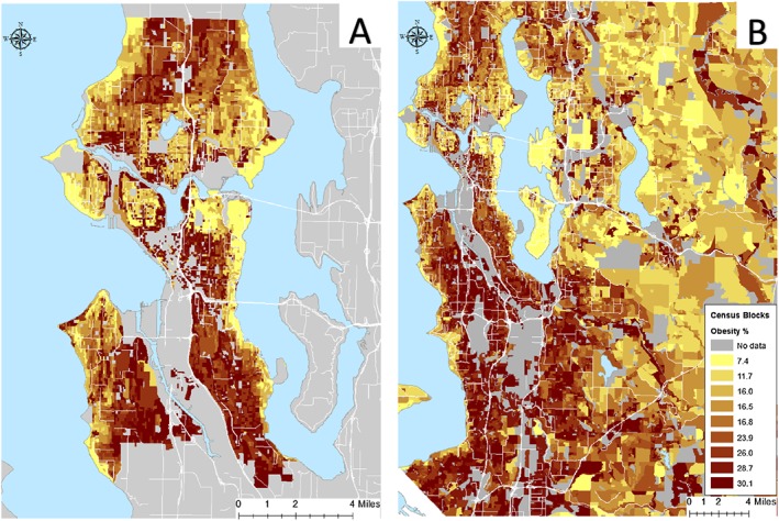
Data visualization for the geographic distribution of obesity prevalence at the census block level for (A) Seattle and King County (B).

Discussion

Modelled obesity prevalence data at a fine granular scale cannot be checked against objective reality, since geo‐located health data are rarely available. The availability of fine‐grained area‐level SES data in Seattle‐King County represents one of the first opportunities to map obesity at a high resolution using empirical, intrinsically geospatial data – residential property values at the tax parcel data. Using these data, maps of the prevalence of obesity and diabetes were previously generated by census tract using data for 59,767 insured persons from Group Health, now Kaiser Permanente 12. The present modelling, at the unprecedented census block level, was generally consistent with past observation and with data collected by the local health authority, Public Health Seattle‐King County.

These data stand in sharp contrast to the RTI International maps for Seattle neighbourhoods 9. Those maps fail to show the expected social gradient in obesity rates 12, 17, showing instead lower obesity prevalence around the freeway corridor and higher prevalence on waterfront estates. One potential explanation is that models that use race and Hispanic origin as the chief predictors of obesity prevalence do little more than highlight long‐standing racial segregation in housing. Such mapping techniques may work where racial divisions in housing are sharply drawn, such as New York City, but may not apply to more integrated Seattle‐King County.

The present modelling approach is based on the premise that socioeconomic disparities are a more powerful determinant of health 18, and one that applies to all racial and ethnic groups. Here, tax parcel property values have multiple advantages as a unifying predictor variable. First, property values are an objective measure that is less prone to omission, misreporting or misclassification 19. Second, property values may better capture economic security, wealth and accumulated assets that do self‐reported incomes 1, 14, 20. In other words, tax parcel property values are an accurate index of social class. Third, tax parcel property values can be geo‐localized with great accuracy to provide indexes of individual or area SES.

This study was not without its limitations. First, the cross‐sectional nature of this analysis precludes any causal inferences between SES and obesity. Second, obesity was calculated based on self‐reported height and weight. Third, the present geographic information system model was based on a single variable at the tax parcel level and did not draw on additional census data that may be available at a higher level of aggregation 8. US Census bureau data are not currently available at tax parcel level. Fourth, obesity prevalence estimates were based on small samples, which may have led to estimate instability. Fifth, although the telephone survey was based on Centers for Disease Control and Prevention Behavioral Risk Factor Surveillance System methodology, we cannot rule out the possibility of selection bias in our sample given that the respondent had to (i) have access to a working telephone, (ii) speak English and (iii) be home when the survey was fielded. However, our sample demographics are similar to 2008 US Census Bureau American Community Survey 3‐year estimates for occupied households in King County and Seattle 75.2% and 74.8% White, non‐Hispanic, 77.3% and 82.6% with a college education or more compared with 81% White, non‐Hispanic and 82.5% with a college education or more in our study sample 21. It should be noted that these American Community Surveys estimate all for residents of Seattle and King County and are not restricted to adults only. When compared with local area Behavioral Risk Factor Surveillance System, our demographics match closely 1. Lastly, the population of Seattle and King County is more educated and affluent, compared with the rest the nation and may not be generalizable to national statistics on obesity.

Conclusion

Neighbourhood maps of US obesity can be created using property values as opposed to age, gender, race, Hispanic origin or educational attainment. Residential property values may become the preferred predictor of socioeconomic disparities in health.

Conflict of interest statement

We have no conflicts of interest to disclose.

Drewnowski, A. , Buszkiewicz, J. , Aggarwal, A. , Cook, A. , and Moudon, A. V. (2018) A new method to visualize obesity prevalence in Seattle‐King County at the census block level. Obesity Science & Practice, 4: 14–19. doi: 10.1002/osp4.144.

References

- 1. Drewnowski A, Aggarwal A, Rehm C. Environments perceived as obesogenic have lower residential property values. Am J [Internet]. 2014 [cited 2017 Jun 4];47(3):260–74. Available from: http://www.sciencedirect.com/science/article/pii/S0749379714001986 [DOI] [PMC free article] [PubMed]
- 2. Zhang Q, Wang Y. Trends in the association between obesity and socioeconomic status in US adults: 1971 to 2000. Obes Res [Internet]. 2004 [cited 2017 Jun 4];12(10):1622–32. Available from: http://onlinelibrary.wiley.com/doi/10.1038/oby.2004.202/full [DOI] [PubMed]
- 3. Panczak R, Held L, Moser A, Jones P. Finding big shots: small‐area mapping and spatial modelling of obesity among Swiss male conscripts. BMC [Internet]. 2016 [cited 2017 Jun 4];3(1):10. Available from: https://bmcobes.biomedcentral.com/articles/10.1186/s40608‐016‐0092‐6 [DOI] [PMC free article] [PubMed]
- 4. Xu Y, Wen M, Wang F. Multilevel built environment features and individual odds of overweight and obesity in Utah. Appl Geogr [Internet]. 2015 [cited 2017 Jun 4];60(197):203. Available from: http://www.sciencedirect.com/science/article/pii/S0143622814002343 [DOI] [PMC free article] [PubMed]
- 5. Koh K, Grady S, Vojnovic I. Using simulated data to investigate the spatial patterns of obesity prevalence at the census tract level in metropolitan Detroit. Appl Geogr [Internet]. 2015 [cited 2017 Jun 4];62(19):28. Available from: http://www.sciencedirect.com/science/article/pii/S014362281500082X
- 6. Huang R, Moudon A, Cook A. The spatial clustering of obesity: does the built environment matter? J Hum [Internet]. 2015 [cited 2017 Jun 4];28(6):604–12. Available from: http://onlinelibrary.wiley.com/doi/10.1111/jhn.12279/full [DOI] [PubMed]
- 7. Mokdad A, Ford E, Bowman B, Dietz W, Vinicor F. Prevalence of obesity, diabetes, and obesity‐related health risk factors, 2001. Jama [Internet]. 2003 [cited 2017 Jun 4];289(1):76–9. Available from: http://jamanetwork.com/journals/jama/fullarticle/195663 [DOI] [PubMed]
- 8. Centers for Disease Control and Prevention . Methods and references for county‐level estimates and ranks and state‐level modeled estimates [Internet]. [cited 2017 Jun 4]. Available from: https://www.cdc.gov/diabetes/pdfs/data/calculating‐methods‐references‐county‐level‐estimates‐ranks.pdf
- 9. Research Triangle Institute International . Neighborhood map of U.S. Obesity [Internet]. [cited 2017 Jun 4]. Available from: http://synthpopviewer.rti.org/obesity/viewer.html
- 10. Drewnowski A, Moudon A, Jiao J. Food environment and socioeconomic status influence obesity rates in Seattle and in Paris. Int J [Internet]. 2014 [cited 2017 Jun 4];38(2):306–14. Available from: http://www.nature.com/ijo/journal/v38/n2/abs/ijo201397a.html [DOI] [PMC free article] [PubMed]
- 11. Jiao J, Drewnowski A, Moudon AV, Aggarwal A, Oppert J‐M, Charreire H, et al. The impact of area residential property values on self‐rated health: a cross‐sectional comparative study of Seattle and Paris. Prev Med Reports [Internet]. 2016 Dec [cited 2017 Aug 7];4:68–74. Available from: http://linkinghub.elsevier.com/retrieve/pii/S2211335516300389 [DOI] [PMC free article] [PubMed]
- 12. Drewnowski A, Rehm CD, Arterburn D. The geographic distribution of obesity by census tract among 59 767 insured adults in King County, WA. Int J Obes [Internet]. 2014; 38: 833–839. Available from: http://www.pubmedcentral.nih.gov/articlerender.fcgi?artid=3955743&tool=pmcentrez&rendertype=abstract. [DOI] [PMC free article] [PubMed] [Google Scholar]
- 13. Drewnowski A, Moudon AV, Jiao J, Aggarwal A, Charreire H, Chaix B. Food environment and socioeconomic status influence obesity rates in Seattle and in Paris. Int J Obes (Lond) [Internet]. 2014; 38: 306–314. Available from: http://www.scopus.com/inward/record.url?eid=2-s2.0-84896696392&partnerID=tZOtx3y1. [DOI] [PMC free article] [PubMed] [Google Scholar]
- 14. Drewnowski A, Aggarwal A, Cook A, Stewart O, Moudon AV. Geographic disparities in Healthy Eating Index scores (HEI‐2005 and 2010) by residential property values: findings from Seattle Obesity Study (SOS). Prev Med (Baltim) [Internet]. 2016;83:46–55. Available from: http://dx.doi.org/10.1016/j.ypmed.2015.11.021 [DOI] [PMC free article] [PubMed]
- 15. ESRI . ArcGIS desktop: release 10 [Internet]. Redlands, CA: Environmental Systems Research Institute; 2011 [cited 2017 Jun 19]. Available from: https://gis.stackexchange.com/questions/5783/how‐do‐you‐cite‐arcgis
- 16. StataCorp . Stata Statistical Software: release 14. College Station, TX: StataCorp LP.; 2015.
- 17. Drewnowski A, Aggarwal A, Cook A, Stewart O. Geographic disparities in Healthy Eating Index scores (HEI–2005 and 2010) by residential property values: findings from Seattle Obesity Study (SOS). Preventive [Internet]. 2016 [cited 2017 Jun 4];83:46–55. Available from: http://www.sciencedirect.com/science/article/pii/S0091743515003576 [DOI] [PMC free article] [PubMed]
- 18. Grossman M. On the concept of health capital and the demand for health. J Polit Econ [Internet]. 1972 [cited 2017 Jun 4];80(2):223–55. Available from: http://www.journals.uchicago.edu/doi/pdfplus/10.1086/259880
- 19. Braveman P, Cubbin C, Egerter S, Chideya S. Socioeconomic status in health research: one size does not fit all. Jama [Internet]. 2005. [cited 2017 Jun 4];294(22):2879–88. Available from: http://jamanetwork.com/journals/jama/fullarticle/202015 [DOI] [PubMed]
- 20. Moudon A, Cook A, Ulmer J, Hurvitz P. A neighborhood wealth metric for use in health studies. Am J [Internet]. 2011 [cited 2017 Jun 4];41(1):88–97. Available from: http://www.sciencedirect.com/science/article/pii/S0749379711002029 [DOI] [PMC free article] [PubMed]
- 21. U.S. Census Bureau , 2006. ‐2008 American Community Survey 3‐year estimates: demographic characteristics for occupied housing units ‐ Seattle and King County.