The Moral Hazard Effects of Consumer Responses to Targeted Cost-Sharing

Abstract

This paper examines the effects of the reference pricing program implemented by the California Public Employees Retirement System (CalPERS) in 2012. The program uses targeted cost-sharing to incentivize patient price shopping. We find that the program leads to a 10.3% increase in the use of low-price providers and reduces the average cost per procedure by 12.5%. We further estimate that the program reduces price-margin medical spending by $218.8 per procedure, which we estimate is approximately 53.7% of the excessive spending that is due to patient choice of higher price providers caused by insurance coverage, at the expense of a $94.3 (or 12.5%) reduction in consumer surplus. The cost savings from the reference pricing program is about two to three times as large as the reduction from implementing a high-deductible health plan while the accompanying consumer surplus reduction is much smaller under reference pricing.

1 Introduction

In response to rising health care spending, many employers and insurers have recently adopted innovative benefit designs as a means to reduce health care costs. These programs are often implemented in response to what economists have known for several decades: generous insurance coverage distorts patient choices. This distortion, commonly referred to as moral hazard, leads to a sizable deadweight loss (Frick & Chernew, 2009). The RAND Health Insurance Experiment (HIE) estimated that full insurance coverage increases medical spending by approximately 20% (Manning et al., 1987). Although the HIE study was conducted several decades ago, the results have been remarkably consistent with more recent studies (Baicker & Goldman, 2011).

Many recent insurance benefit designs are designed to limit the moral hazard effects of traditional insurance coverage by reducing the generosity of coverage. There are various types of moral hazard, one of which is the tendency to demand care from a more expensive provider. This paper examines how a particular benefit design innovation pioneered by one of the largest purchasers of health insurance in the United States reduces the use of more expensive providers, an important dimension of moral hazard that has not been previously studied. In particular, we examine how the reference pricing program implemented by the California Public Employees Retirement System (CalPERS) for colonoscopy services spurs price shopping. We find that the program leads to substantial reductions in spending along the intensive margin, which we define as the price of each procedure, as patients switch demand to lower-priced providers.¹

The most common benefit design change, high-deductible health plans (HDHPs) attempts to reduce moral hazard by substantially increasing initial patient cost-sharing while still protecting against catastrophic risks. While the initial hope was that by giving consumers “skin in the game” HDHPs would spur price shopping for health care services, recent evidence finds that nearly all of the consumer responses come through decreased utilization of care (Brot-Goldberg et al., 2015; Haviland et al., 2016). This evidence is not inconsistent with the HIE. Both the RAND experiment and nearly all subsequent studies have examined the effect of insurance coverage on total medical spending rather than on price shopping. In general, the price elasticities estimated by the RAND HIE and other studies consist of price sensitivities along both the extensive, the decision to receive care, and the intensive, the price paid conditional on receiving care, margins. This paper is among the first to make a distinction between these two components of price sensitivity and to focus explicitly on the latter component-how does insurance coverage impact where patients receive care and the price of that care?

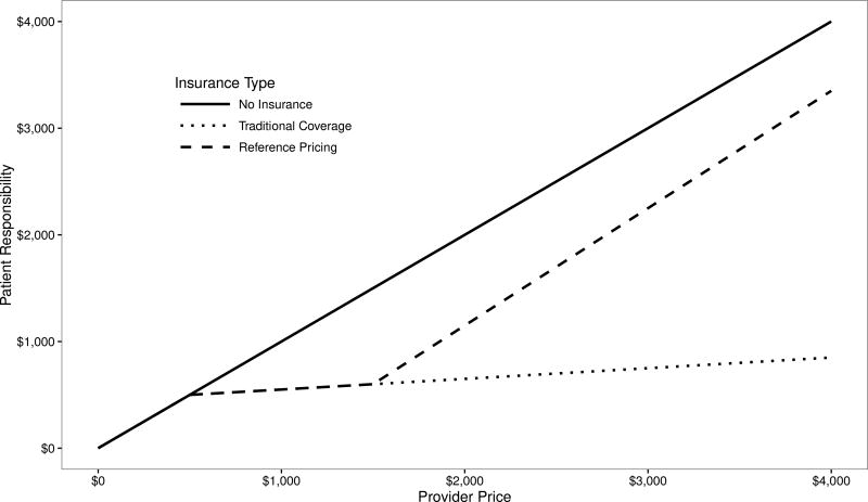
To examine this question, we leverage data from an innovative program that uses strong financial incentives to direct patients to low-priced providers. In 2012, CalPERS implemented a program that limits reimbursement for care received at high-priced providers. This program sets a “reference price” for common outpatient surgical services, in this case, $1,500 for colonoscopies. Figure 1 presents a stylized example of how reference pricing changes consumer cost-sharing. Without insurance coverage, the solid line, consumers are responsible for the entire marginal cost of care. Under both traditional insurance coverage, the dotted line, and reference pricing, the dashed line, patients are responsible for the full cost up to the $500 deductible, and then a 20% coinsurance. However, under reference pricing, above the $1,500 price threshold, patients are responsible for the full difference in prices between the provider’s price and the reference price. Due to this construction, the reference pricing program provides a strong incentive for patients to respond to provider price variation.

Figure 1.

Reference Pricing Illustration

This mechanism is in contrast to HDHPs, under which patients have little financial incentive to respond to price variation in surgical services, since much of the variation in prices occurs at prices that typically exceed most deductibles. The underlying intuition of reference pricing is analogous to “balance billing” policies allowed for non-participating providers under Medicare. Under balance billing, patients are responsible for the difference between a provider’s price and the Medicare reimbursement amount, up to a maximum of 9.25% above the approved Medicare fee schedule for non-participating providers (MedPAC, 2016). Similarly, under the CalPERS reference pricing program, the maximum amount that a provider can charge beyond the reference price is the negotiated price between the insurer and the provider, which will vary across providers and is negotiated annually.

By focusing on the price of received care in response to the policy change, this program leads to large consumer responses. For colonoscopy services, the focus of this paper, a previous study shows that by shifting demand from high-priced to low-priced providers, reference pricing saved CalPERS $7 million over two years (Robinson et al., 2015a). Aouad et al. (2017b) finds that the program leads to an approximately 67% increase in the probability of total costs being below the reference price threshold for the patients who switch and Aouad et al. (2017a) uses a quantile-treatment approach and finds that the majority of the savings occur from the right tail of the price distribution. This paper extends the results of these studies. We find that the program increased demand for low-priced providers, which reduced the average cost per-procedure by approximately 12%. However, there is an approximately 31% increase in patient cost-sharing.

We then estimate the reduction in spending and consumer surplus due to the program. Our model shows that the magnitude of the demand and spending difference between the reference pricing program and traditional coverage depends on own-price elasticities with respect to consumer cost-sharing. We use a discrete choice model to estimate how the program changes consumer choice of surgical providers. Using the reference pricing program as an exogenous shock to patient cost-sharing, we estimate that the Aggregated Direct Elasticity (ADE) of out-of-pocket spendings ranges from −0.38 to −1.93, depending on the heterogeneity in provider prices. The price shopping elasticity estimates of our models and estimates on other product attributes allow us to estimate the magnitude of consumer surplus reduction compared to a standard benefit design. Across all colonoscopies received by CalPERS patients following the implementation of the reference pricing program, we estimate that the program leads to a per-procedure reduction of $218.8 in spending and a $94.3 reduction in consumer surplus. We further estimate that this reduction accounts for approximately 53.7% of the excessive spending due to patient choice of more expansive providers under insurance coverage than when they are not insulated from prices by insurance. The accompanying reduction in consumer surplus accounts for only 12.5%.

Finally, we use the structural parameters from our choice model to estimate the spending difference and consumer surplus difference from two alternative reference prices–lowering the reference price to $1,000 and increasing it to $2,000–and three high-deductible plans (a deductible of $1,500, $3,000 and $5,000). Each alternative reference prices scenario shows similar effects as the actual $1,500 reference price. Intuitively, patients are relatively insensitive to the increased cost-sharing near the reference price. Not until the $2,500 price point do consumers change demand. Thus, any localized change in the reference price doesn’t lead to substantial changes in consumer behavior but simply changes the amount of the provider’s price that is shifted to consumers. But the cost saving from reference prices is about two to three times as large as the cost saving from implementing a HDHP. At the same time, we also estimate that HDHPs lead to a greater reduction in consumer surplus.

The paper proceeds as follows. Section 2 provides an overview of the CalPERS program and previous studies of both moral hazard in health insurance and the effects of the CalPERS program. Section 3 describes the data used for this study. Section 4 provides reduced form evidence of the consumer responses to the program. Section 5 presents and estimates the structural model, Section 6 estimates counterfactuals, and Section 7 concludes.

2 Institutional Background

The California Public Employees Retirement System (CalPERS), provides health insurance benefits to California state and municipality employees, retirees, and their dependents. With approximately 1.4 million enrollees, CalPERS is the second largest purchaser of commercial health insurance in the United States. CalPERS applied reference pricing to its Anthem Blue Cross PPO plans, which provides benefits for approximately 225,000 enrollees, with the remaining CalPERS enrollees being covered by various HMO or Medicare options. In 2011, CalPERS implemented reference pricing for knee and hip replacement surgeries after noticing an approximate six-fold variation in negotiated prices (from $20,000 to $120,000) with no correlation between facility prices and either surgical quality or complication rates. As a way of providing targeted incentives for patients to receive care from the less expensive providers, CalPERS implemented a reference price, also known as a reimbursement limit, of $30,000. Patients receiving care from providers with negotiated rates above $30,000 were responsible for the entire difference in the provider’s price and the reimbursement limit. Prior to the reference pricing program, patients were responsible for a deductible of $500 or $1,000, depending on their specific PPO plan choice, and a coinsurance rate of 20%. The move from this traditional insurance coverage to reference pricing led to a 20% reduction in procedure costs for these two services, which saved CalPERS $3 million over two years (Robinson & Brown, 2013).

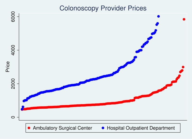
After successfully implementing reference pricing for these joint replacement surgeries, CalPERS expanded the program to outpatient services (colonoscopy, cataract replacement surgery, and joint arthroscopy surgeries) in 2012. These services have similar degrees of price dispersion and no measurable relationship between price and quality. Like knee and hip replacement surgery, these outpatient services are considered “shoppable.” Services are “shoppable” if they are not immediately required (e.g., not emergency services), quality varies little across providers, and patients can accurately differentiate between low-price and high-price providers. In addition, many ambulatory surgical centers (ASCs), which are not hospital-based, provide these services. As a results, ASCs typically have lower prices than hospital outpatient departments (HOPDs). Figure 2 shows this difference by plotting the mean 2011 price for each provider. Each point in this figure represents the mean 2011 price for a distinct ASC or HOPD provider. In 2011, the mean price for a colonoscopy received at a HOPD was $3,026. The mean price for a colonoscopy received at an ASC was approximately one-third as expensive, $1,047.

Figure 2.

Distribution of Colonoscopy Provider Prices

This figure plots the distribution of colonoscopy prices for CalPERS patients in 2011. The red points show prices for Ambulatory Surgical Center (ASC) providers while the blue points show prices for Hospital Outpatient Departments (HOPDs).

To make the expanded reference pricing program easier to understand, CalPERS only instituted reimbursement limits for services received at HOPDs: $1,500 for colonoscopy, $2,000 for cataract surgery, and $6,000 for joint arthroscopy. Patients receiving care from an ASC are only subject to the standard cost-sharing of deductibles and coinsurance, regardless of the ASC’s price, which will only rarely be greater than the reference price applied to HOPDs. For cataract replacement surgery, the expanded reference pricing program reduced average procedure costs by 17.9% and reduced CalPERS medical spending by $1.3 million over two years (Robinson et al., 2015c). For arthroscopic surgery, the expanded program reduced average procedure costs by 17.0% for shoulder arthroscopy and 17.6% for knee arthroscopy, saving CalPERS $2.3 million over two years Robinson et al. (2015b).

While the existing studies document the financial savings for the reference pricing programs, they do not fully document the scope of consumer choices. Although the existing studies show that consumers shift demand from HOPDs to ASCs, they do not examine if patients also shift to less expensive HOPDs. This aspect is important to consider when evaluating how consumers understand the program. The existing studies also do not examine how consumers incorporate provider location, quality, and other non-price attributes into their provider choices. To incorporate the attributes, we use the same natural experiment used in the previously discussed reference pricing papers but use a discrete choice model to better understand how reference pricing influences the full spectrum of provider choices. Our consumer demand model allows us to better understand the nature of the reference pricing program and to estimate the reductions in excessive spending and consumer surplus resulting from the reference pricing program.

2.1 Literature

This paper follows the long health economics literature on cost-sharing as a means to reduce the moral hazard inherent with insurance coverage (Arrow, 1963; Pauly, 1968; Feldstein, 1973; Feldman & Dowd, 1991; Cutler & Zeckhauser, 2000; Baicker & Goldman, 2011; Kowalski, 2012; Einav et al., 2013). Medical spending increases due to insurance coverage can occur along the extensive margin, whether to use any medical care at all (or whether to use a particular subset of medical care), or along the intensive margin, a change in medical expenditures, given that a patient has already chosen to receive medical care. Patient behavior on the intensive margin can be further decomposed into patient behavior regarding utilization and patient price shopping. We restrict the intensive margin to patient choice of provider, price shopping, rather than quantity because patients are unlikely to multiple units of the same service during the same visit.² Traditional economic models have focused primarily on the extensive margin, the decision to receive care, and have focused less on patient price search behavior along the intensive margin.

At the same time, much of the recent empirical literature has focused on the moral hazard effects of high-deductible health plans (HDHP), which require patients to bear the full burden of initial spending before insurance coverage is applied. Because patients are responsible for a substantial portion of medical spending, high-deductible and other traditional cost-sharing plans should theoretically address moral hazard on both margins. However, evidence suggests that traditional cost-sharing only addresses moral hazard on the extensive margin. HDHPs lead to an overall reduction in utilization but do not lead patients to receive care from less expensive providers (Sood et al., 2013; Huckfeldt et al., 2015; Brot-Goldberg et al., 2015; Haviland et al., 2016).

More recently, narrow network insurance plans focused exclusively on the intensive margin moral hazard problem by simply excluding expensive providers from the insurance network. Patients receiving care at an excluded provider are responsible for the entire price. Gruber & McKnight (2016) find that the narrow network plan offered by the Massachusetts Group Insurance Commission, the Massachusetts equivalent to CalPERS, successfully provided incentives for patients to visit less expensive providers. Likewise, Frank et al. (2015) find that a tiered cost-sharing design for inpatient hospitalizations leads to a 7.6 percentage point shift in demand from high-priced to low-priced providers. Similar work has focused on the price and utilization effects of the Medicare Part D coverage gap. The Part D literature is especially relevant to reference pricing due to the non-linear cost-sharing (Joyce et al., 2013; Einav et al., 2015). Like reference pricing, the Part D coverage gap imposes full cost-sharing following a period of full coverage. Many Part D plans are even more similar to reference pricing by offering coverage for low-cost generic drugs.

The reference pricing program we study combines these approaches to reducing moral hazard. Like narrow network and tiered benefit insurance plans, it operates on the price shopping aspect of the intensive margin by providing incentives for individuals to receive less expensive care rather than reduce their utilization of care. In effect, reference pricing serves to make patients more responsive to the prices of expensive providers.³ Our data construction allows us to empirically measure the degree of price sensitivity using the exogenous out-of-pocket spending increase caused by the non-linear benefit coverage of the reference pricing program. We further estimate the change in spending and consumer surplus caused by the program.

3 Data

To estimate the effects of the CalPERS program we use medical claims data from an Anthem Blue Cross of California PPO plan. Important to this paper, the Anthem PPO consists of two patient populations. The first population consists of CalPERS patients enrolled in the Anthem PPO plan. CalPERS patients in the sample were exposed to the reference pricing program starting in January, 2012. Our second patient population consists of non-CalPERS patients enrolled in an Anthem PPO that did not include a reference pricing program. Because Anthem administers each population’s benefits, each in-network provider’s negotiated prices are the same for both groups. This aspect makes the non-CalPERS population an ideal control group for the CalPERS population.

For both populations, we use claims data for colonoscopy services covering the years 2009–2013 and thus include three years before the program’s implementation and two years following implementation. While the reference pricing program also applies to joint replacement surgery, joint arthroscopy, and cataract surgery, we restrict the analysis to colonoscopy services because colonoscopies are by far the most common of the reference-priced services.⁴

As with other medical claims data, this data includes basic demographic information (patient age, gender, and zip code), the date of service, the facility performing the service, and the cost of the service, which is separated by consumer cost-sharing and employer spending. To measure prices, we use the sum of the consumer and employer spending, which is commonly referred to as the “allowed amount” of the service. The data also contains information on patient comorbidities and diagnosis codes for one year prior to each patient’s colonoscopy, which we use to construct Charlson comorbidity scores (Charlson et al., 1987).

Table 1 also presents the descriptive characteristics of each population. The two populations have similar demographic characteristics. Similar shares of each population received care at HOPDs in the period before the implementation of CalPERS’ reference pricing program. Although each patient faces the same price at any given facility, the CalPERS population has slightly higher average prices than the control population. These higher average prices reflect the larger shares of CalPERS enrollees located in the Northern California region, which is more concentrated and typically has higher prices, than the more competitive Southern California regions.

Table 1.

Summary Statistics

	2009	2010	2011	2012	2013
Panel A: all colonoscopy
Mean insurer paid amount
Anthem	946.60	999.73	1136.00	1274.86	1356.46
CalPERS	1238.13	1327.90	1511.34	1322.43	1397.00
Mean patient responsibility
Anthem	786.08	881.84	961.91	999.76	1223.04
CalPERS	469.96	546.94	494.14	725.74	778.59
Average Charlson Score
Anthem	0.13	0.13	0.13	0.12	0.12
CalPERS	0.14	0.14	0.13	0.12	0.13
Percent male
Anthem	46.64%	46.55%	46.60%	46.73%	46.80%
CalPERS	45.09%	44.16%	44.38%	43.56%	42.76%
Mean age
Anthem	52.52	52.62	52.67	52.72	52.89
CalPERS	54.47	54.70	54.83	54.66	54.91
ASC share
Anthem	71.31%	71.75%	72.66%	72.83%	72.02%
CalPERS	66.76%	67.05%	66.18%	74.00%	76.08%
Number of procedures
Anthem	56099	53417	53680	57027	60687
CalPERS	8369	8163	8188	7904	7292
Panel B: colonoscopy in mixlogit analysis
Mean insurer paid amount
Anthem	705.61	732.14	808.10	909.33	1009.26
CalPERS	929.00	945.76	1405.05	1104.11	1125.07
Mean patient responsibility
Anthem	443.16	474.16	547.93	570.23	556.08
CalPERS	293.85	333.87	414.42	485.16	442.58
Average Charlson Score
Anthem	0.11	0.11	0.12	0.12	0.12
CalPERS	0.14	0.17	0.18	0.17	0.14
Percent male
Anthem	47.69%	47.54%	47.55%	48.03%	47.09%
CalPERS	45.55%	44.35%	40.24%	43.70%	40.18%
Mean age
Anthem	52.35	52.38	51.76	51.02	51.19
CalPERS	53.62	53.88	52.43	52.35	52.5
ASC share
Anthem	76.43%	77.02%	74.87%	74.32%	74.31%
CalPERS	75.34%	75.72%	57.62%	68.61%	75.04%
Number of procedures
Anthem	22265	21776	15423	14300	14117
CalPERS	2283	2088	984	1405	1222

4 Reduced Form Evidence

4.1 Difference-in-Differences Empirical Strategy

We start by estimating difference-in-differences regressions that measure the overall effects of the program. For these regressions we use six outcome variables. The first is the price per colonoscopy service. This price is the bundled “allowed amount” that includes both patient cost-sharing and payments by the employer or insurer. This price represents the price to which the reference pricing program was applied. Second, to estimate the effects of the program on patient spending, we include the amount paid by the patient. This amount includes traditional cost-sharing (the sum of deductible and coinsurance amounts) up to the reference price and the additional “surcharge” (provider price less the reference price) applied to CalPERS members who receive care from high-priced providers following the program’s implementation. Third, to estimate the effects on spending by CalPERS, we include the amount spent on each colonoscopy by employers, which is the allowed amount less patient cost-sharing. Fourth, to measure changes in patient choice of colonoscopy provider, we also measure the dichotomous outcome of receiving care at a covered provider (either an ASC or HOPD with a price below the $1,500 reference price) or a non-covered provider (HOPD with a price above the reference price). Our final to outcomes measure changes in non-price attributes that could be impacted by the program. We measure the risks of procedural complications related to the colonoscopy procedure. The procedural complications include outcomes such as intestinal perforations, cardiac events, and stomach pain.⁵ We also measure the distance between the zip code of the patient and the provider from which they receive care. We measure the total price, patient cost-sharing, employer spending, and distance in logarithmic units.

With each outcome_it, we estimate

$${\mathit{\text{outcome}}}_{\mathit{\text{it}}}=\alpha +{\beta }_1{\mathit{\text{CalPERS}}}_i+{\delta }_{\mathit{\text{DD}}}{\mathit{\text{CalPERS}}}_i\times {\mathit{\text{post}}}_t+X_i+\tau {\mathit{\text{year}}}_t+{\epsilon }_{\mathit{\text{it}}}.$$ (1)

In this model, CalPERS_i identifies CalPERS patients, post_t is a dummy for the period following the 2012 implementation. The year fixed effects negate the need for the main post_t effect. The coefficient on the interaction term, δ_DD, captures the effects of the program. For each outcome, it measures the difference in the before and after 2012 change relative to the change in the non-CalPERS population. X_i controls for patient demographics (age, gender, Charlson comorbidity score). To account for market effects and market-specific time trends, we iteratively add fixed effects for Hospital Referral Regions (HRRs) and HRR by year fixed effects. We estimate each regression using OLS and cluster the standard errors at the patient HRR-level.

4.2 Difference-in-Differences Results

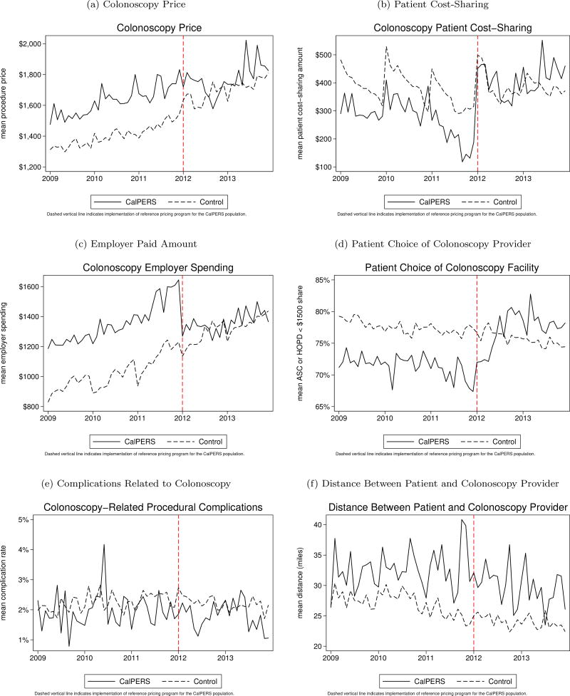
Figure 3 presents unadjusted trends in each of the six outcomes between the CalPERS (solid line) and non-CalPERS (dashed line) population. For each outcome, the trends between the CalPERS and non-CalPERS population are similar until 2012, which is indicated in each figure by the dashed vertical line. After 2012 and relative to the non-CalPERS population, the CalPERS population experiences a reduction in the average price per colonoscopy and in employer spending on colonoscopies. There is an increase in patient cost-sharing and the probability of receiving care from either an ASC or a HOPD with a price below $1,500. We do not see evidence of any change in the rate of procedural complications or distance travelled.

Figure 3.

Unadjusted Trends

The regression results support the visual evidence presented by the unadjusted trends. For total spending, the results in Table 2 suggest that the program leads to a sizable reduction in colonoscopy costs. Depending on the inclusion of HRR and HRR by year fixed effects, the effect size ranges from a 11.3% to 12.5% reduction in per-procedure costs for the CalPERS population.⁶ At the mean price among CalPES patients in 2011 of $1,716 this effect translates to a $194.0 to $215.2 reduction in the average cost per colonoscopy service. This reduction is slightly smaller than the results found in Robinson et al. (2015a) largely because the Robinson et al. (2015a) results parametrically control for CalPERS patients with an exemption from the reference pricing program, effectively excluding them from influencing the impact of the program, while the current results include all patients. Including the entire population provides an estimate of exposure for the entire CalPERS population in an intent-to-treat framework rather than just a defined subset. We also pool both the 2012 and 2013 treatment effects into one post_t indicator but the treatment effect in the second year of the program is larger than the treatment effect in the first year.

Table 2.

Changes in Colonoscopy Prices

	(1) ln(price)	(2) ln(price)	(3) ln(price)
CalPERS × post	−0.133*** (0.0262)	−0.134*** (0.0251)	−0.120*** (0.0264)
CalPERS	0.191*** (0.0417)	0.121*** (0.0273)	0.115*** (0.0278)
2009	−0.105*** (0.0170)	−0.115*** (0.0159)	0.225*** (0.00572)
2010	−0.0630*** (0.0119)	−0.0715*** (0.0103)	0.116*** (0.00356)
2012	0.108*** (0.0253)	0.113*** (0.0266)	0.226*** (0.0110)
2013	0.143*** (0.0274)	0.153*** (0.0299)	0.231*** (0.0104)
Observations	320,826	320,826	320,826
R2	0.028	0.141	0.148
Mean CalPERS 2011 price	1,716	1,716	1,716
Fixed Effects		HRR	HRR × year

This table presents the difference-in-differences results from equation 1 and uses the log of the total colonoscopy cost as the dependent variable. All columns include controls for patient demographics (age, gender, Charlson risk score), the primary colonoscopy procedure code, and month. Column 2 adds patient HRR fixed effects and column 3 adds year by patient HRR interactions. Robust standard errors clustered at the provider level are in parentheses.

^***p<0.01,

^**p<0.05,

^*p<0.1.

The effects on patient and employer spending are shown in Tables 3 and 4. For patients, we find a price increase that ranges from 25.0% to 30.3% depending on the fixed effects included in each specification. At the mean baseline patient cost-sharing among CalPERS patients of $205, this increase translates into a $51.3 to $62.2 increase in patient cost-sharing. On the other hand, we find that the program leads to a decrease in CalPERS spending that ranges from 17.6% to 20.7%. At the mean baseline CalPERs spending of $1,511, this translates into a $266.5 to $312.9 reduction in reimbursements for colonoscopy services. The increase in patient cost-sharing is not surprising as the reference pricing program explicitly increases cost-sharing for high-priced providers. While a sizable share of patients do switch to the lower-priced alternatives, there is not full compliance with the program.

Table 3.

Changes in Patient Cost Sharing

	(1) ln(patient+1)	(2) ln(patient+1)	(3) ln(patient+1)
CalPERS × post	0.223*** (0.0432)	0.238*** (0.0439)	0.265*** (0.0426)
CalPERS	0.0500 (0.0315)	0.0781*** (0.0214)	0.0671*** (0.0221)
2009	0.0258 (0.0438)	0.0393 (0.0445)	−0.0393 (0.0659)
2010	−0.0117 (0.0233)	−0.0000119 (0.0231)	−0.143*** (0.0502)
2012	0.0943** (0.0439)	0.0842* (0.0434)	0.156*** (0.0364)
2013	0.0872 (0.0539)	0.0704 (0.0516)	0.110*** (0.0171)
Observations	320,826	320,826	320,826
R2	0.771	0.775	0.776
Mean CalPERS 2011 cost-share	205	205	205
Fixed Effects		HRR	HRR × year

This table presents the difference-in-differences results from equation 1 and uses the log of patient spending as the dependent variable. All columns include controls for patient demographics (age, gender, Charlson risk score), the primary colonoscopy procedure code, and month. Column 2 adds patient HRR fixed effects and column 3 adds year by patient HRR interactions. Robust standard errors clustered at the provider level are in parentheses.

^***p<0.01,

^**p<0.05,

^*p<0.1.

Table 4.

Changes in Employer and Insurer Spending

	(1) ln(paid+1)	(2) ln(paid+1)	(3) ln(paid+1)
CalPERS × post	−0.209*** (0.0542)	−0.232*** (0.0494)	−0.194*** (0.0545)
CalPERS	0.799*** (0.0838)	0.671*** (0.0876)	0.657*** (0.0893)
2009	0.0514 (0.0352)	0.0216 (0.0353)	0.953*** (0.0288)
2010	0.0299 (0.0252)	0.00468 (0.0245)	0.601*** (0.0218)
2012	0.135*** (0.0371)	0.155*** (0.0377)	0.479*** (0.0156)
2013	0.226*** (0.0442)	0.260*** (0.0479)	0.454*** (0.0221)
Observations	320,826	320,826	320,826
R2	0.113	0.154	0.156
Mean CalPERS 2011 paid amount	1,511	1,511	1,511
Fixed Effects		HRR	HRR × year

This table presents the difference-in-differences results from equation 1 and uses the log of employer and insurer spending on colonoscopy services (i.e. allowed amount - patient cost-sharing) as the dependent variable. All columns include controls for patient demographics (age, gender, Charlson risk score), the primary colonoscopy procedure code, and month. Column 2 adds patient HRR fixed effects and column 3 adds year by patient HRR interactions. Robust standard errors clustered at the provider level are in parentheses.

^***p<0.01,

^**p<0.05,

^*p<0.1.

Table 5 shows similar results when using provider type as the dependent variable. These results imply an approximately 6.8 to 7.8 percentage point decrease in the probability of receiving care from either an ASC or a HOPD with a price below $1,500, compared to a HOPD with a price above the $1,500 reference price. At the mean baseline rate of 70%, the percentage point reductions translate to a 10.3% to 9.0% decrease in the probability of receiving care at a high-priced HOPD provider. When we use the probability that a patient receives care from an ASC instead of a HOPD, the results are nearly identical. For all three columns, a Wald test fails to reject the equality of the CalPERS_i × post_t between regressions that use the covered provider definition (ASC or HOPD with a price less than $1,500 vs. a HOPD priced above $1,500) or the ASC vs. HOPD dependent variable. The similarity between the regressions with each dependent variable implies that the primary choice of provider is made on the ASC vs. HOPD distinction.

Table 5.

Changes in Patient Choice of Colonoscopy Provider

	HOPD
	(1)	(2)	(3)
CalPERS × post	0.0779*** (0.0142)	0.0777*** (0.0139)	0.0682*** (0.0125)
CalPERS	−0.0647*** (0.0215)	−0.0270** (0.0118)	−0.0229* (0.0129)
2009	0.0160 (0.0110)	0.0232** (0.0110)	−0.149*** (0.00337)
2010	0.00605 (0.00686)	0.0124** (0.00592)	−0.0879*** (0.00242)
2012	(0.0113)	−0.00879 (0.0118)	−0.110***(0.00868)
2013	−0.0182 (0.0176)	−0.0198 (0.0185)	−0.0836*** (0.00285)
Observations	320,826	320,826	320,826
Mean CalPERS 2011 share	0.70	0.70	0.70
Fixed Effects		HRR	HRR × year

This table presents the difference-in-differences results from equation 1 and uses the probability of choosing either an ASC or an HOPD with a price below $1,500 as the dependent variable. All columns include controls for patient demographics (age, gender, Charlson risk score), the primary colonoscopy procedure code, and month. Column 2 adds patient HRR fixed effects and column 3 adds year by patient HRR interactions. Robust standard errors clustered at the provider level are in parentheses.

^***p<0.01,

^**p<0.05,

^*p<0.1.

For the non-price attributes, Table 6, shows no change in the rate of procedural complications related to colonoscopy. All three coefficients are negative, but none of the three are statistically significant. At least along the quality outcomes represented by procedural complications, the lack of an effect suggests that there is little link between price and quality for colonoscopy services. Similarly, in Table 7, we find no effect on the distance travelled between patients and providers. This lack of an effect implies that the program did not cause patients to travel further for colonoscopy services. This result may not be surprising, as the program was intentionally designed to ensure patient access to ASCs. Patients without an ASC within 30 miles of their home address are able to request an exemption from the program.

Table 6.

Changes in Procedural Complications

	(1) complication	(2) complication	(3) complication
CalPERS × post	−0.00227 (0.00159)	−0.00251 (0.00156)	−0.00136 (0.00151)
CalPERS	0.000250 (0.00122)	0.00107 (0.000921)	0.000666 (0.000943)
2009	−0.00253*** (0.000728)	−0.00253*** (0.000727)	0.00208*** (0.000429)
2010	−0.000552 (0.000744)	−0.000575 (0.000753)	0.00441*** (0.000356)
2012	−0.000153 (0.000784)	−0.0000977 (0.000776)	0.00251*** (0.000847)
2013	−0.00169* (0.000906)	−0.00166* (0.000897)	0.00719*** (0.000596)
Observations	320,826	320,826	320,826
R2	0.021	0.021	0.022
Mean CalPERS 2011 complication rate	0.020	0.020	0.020
Fixed Effects		HRR	HRR × year

This table presents the difference-in-differences results from equation 1 and uses the probability of receiving a procedural complication related to colonoscopy as the dependent variable. All columns include controls for patient demographics (age, gender, Charlson risk score), the primary colonoscopy procedure code, and month. Column 2 adds patient HRR fixed effects and column 3 adds year by patient HRR interactions. Robust standard errors clustered at the provider level are in parentheses.

^***p<0.01,

^**p<0.05,

^*p<0.1.

Table 7.

Changes in Distance Travelled

	(1) ln(distance+1)	(2) ln(distance+1)	(3) ln(distance+1)
CalPERS × post	−0.00627 (0.0252)	−0.0245 (0.0255)	−0.0163 (0.0238)
CalPERS	0.0420 (0.0812)	−0.0342 (0.0282)	−0.0367 (0.0289)
2009	0.0206 (0.0231)	−0.00870 (0.0167)	0.0779*** (0.00639)
2010	0.0446** (0.0183)	0.0150 (0.0120)	0.0505*** (0.00573)
2012	−0.00773 (0.0117)	0.00428 (0.0109)	0.350*** (0.0121)
2013	−0.00586 (0.0260)	0.0178 (0.0227)	0.771*** (0.00613)
Observations	320,826	320,826	320,826
R2	0.004	0.130	0.133
Mean CalPERS 2011 distance	33	33	33
Fixed Effects		HRR	HRR × year

This table presents the difference-in-differences results from equation 1 and uses the distance between the patient’s zip code and the provider’s zip code as the dependent variable. All columns include controls for patient demographics (age, gender, Charlson risk score), the primary colonoscopy procedure code, and month. Column 2 adds patient HRR fixed effects and column 3 adds year by patient HRR interactions. Robust standard errors clustered at the provider level are in parentheses.

^***p<0.01,

^**p<0.05,

^*p<0.1.

4.2.1 Robustness

In Appendix Tables A.1 to A.6, we estimate the same regressions but test for parallel time trends between the CalPERS and non-CalPERS populations. We replace the CalPERS_i × post_t variable with four yearly interactions that test the difference between the CalPERS and non-CalPERS population in each year. We use 2011, the year prior to implementation, as the reference year. For overall colonoscopy prices, we find a small increase in prices for the CalPERS population in 2010. However, in 2012 and 2013, this trend reverses and the average cost for a CalPERS patient is considerably lower than for a non-CalPERS patient. In, Table A.2, we find that patient cost-sharing increased by approximately 7–10% relative to the non- CalPERS population. Following implementation of reference pricing, patient cost-sharing for CalPERS patients increased by approximately 25–32% more than for non-CalPERS patients. Table A.3 shows that in the two pre-implementation years, the employer paid amount was higher for the CalPERS patients. Following implementation, CalPERS paid approximately 15% less for colonoscopy services than did non-CalPERS employers. Table A.4 shows no pre-implementation difference in the choice of covered providers (ASC or HOPD priced below $1,500) vs. non-covered providers (HOPD priced above $1,500) between the CalPERS and non-CalPERS populations. Finally, Tables A.5 and A.6 do not show a difference in complication rates or distance travelled between the CalPERS and non-CalPERS populations in either the pre-implementation or post-implementation periods.

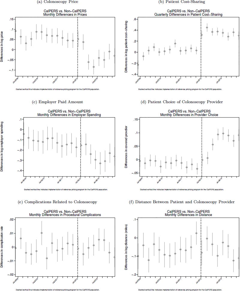
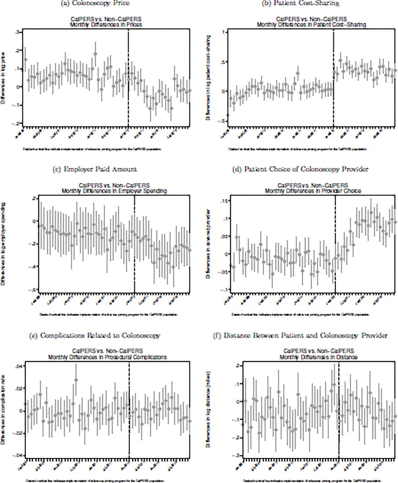
Similarly, Appendix Figure A.1 presents the quarterly differences in each outcome between the CalPERS and non-CalPERS populations. Appendix Figure A.2 plots the monthly differences between the two populations. Each figure plots the CalPERS_i indicators from set of regressions that are restricted to each time period (i.e. each quarter or month). For each outcome, we do not find meaningful pre-implementation trends. However, for the colonoscopy price, patient cost-sharing, employer paid amount, and patient choice of provider outcomes, we do see an immediate impact following implementation relative to the non-CalPERS population.

5 Structural Model

To estimate the structural model, we use the following discrete choice framework. In this model, each consumer i receives at least one unit of care from a set of providers j ∈ J. We assume a linear utility function where choices are a function of provider non-price and price attributes:

$$U_{\mathit{\text{ij}}}=\underset{{\delta }_{\mathit{\text{ij}}}}{\underbrace{\gamma {\mathit{\text{quality}}}_j+\eta {\mathit{\text{OOP}}}_{\mathit{\text{ij}}}(p_j)+\rho {\mathit{\text{quality}}}_j+\varphi {\mathit{\text{distance}}}_{\mathit{\text{ij}}}+\psi {\mathit{\text{HOPD}}}_j}}+{\epsilon }_{\mathit{\text{ij}}}.$$ (2)

Under standard utility maximization, patient i will receive care from provider j if and only if U_ij ≥ U_i,−j∀− j ≠ j. In this model, we include both non-price (provider quality, the distance between the patient’s and provider’s zip codes, and an indicator for whether the provider is a HOPD or ASC) and price attributes that likely influence patient choice of provider.

Our cost-sharing measure OOP_ij(p_j) measures the expected patients out-of-pocket cost for receiving care and is a function of the provider’s price, p_j, the patient’s remaining amount on their deductible, D_i, and coinsurance, α. In our data, with the exception of the CalPERS population receiving care at an HOPD in 2012–2013, OOP_ij(p_j) = D_i + α(p_j − D_i). For the CalPERS population subject to reference pricing who receive care at an HOPD in 2012–2013, cost-sharing is given by the following schedule:

$${\mathit{\text{OOP}}}_{\mathit{\text{ij}}}(p_j)=\{\begin{array}{cc}{D}_i+\alpha (p_j-D_i)\hfill & \text{if }{p}_j\le R\hfill \\ D_i+\alpha (R-D_i)+p_j-R\hfill & \text{if }{p}_j>R\hfill \end{array}$$ (3)

This expression makes clear the intention of the reference pricing program. For prices below the reference price, there is no cost-sharing difference between the reference pricing program and traditional insurance designs. However, at prices above R, patients are responsible for the full marginal price. Thus, above R, insurance coverage offers no insulation from provider prices. How this exposure to the full marginal price changes patient choices is the focus of the rest of the paper.

5.1 Demand Model

To illustrate how the reference pricing changes demand and the welfare implications of these changes in demand, we consider three insurance coverage scenarios. First, we consider the case of no insurance, which we denote as U^U. In the demand function of equation 2, we simply replace OOP_ij(p_j) with the full price.

$$U_{\mathit{\text{ij}}}^U=\gamma {\mathit{\text{quality}}}_j+\eta p_j+\rho {\mathit{\text{quality}}}_j+\varphi {\mathit{\text{distance}}}_{\mathit{\text{ij}}}+\psi {\mathit{\text{HOPD}}}_j+{\epsilon }_{\mathit{\text{ij}}}.$$

The second scenario we consider is the case of traditional coverage, U^TC, where patients are subject to deductibles and coinsurance. In this case, OOP_ij(p_j) = D_i + α(p_j − D_i). The final scenario we consider is reference pricing, U^RP, where out-of-pocket costs are given in equation 3.

We next calculate the changes in patient i’s utility for choosing provider j relative to a reference provider j′ under each insurance scenario, which will be a measure of relative demand. This change in relative demand occurs along the intensive margin as we are assuming that each patient still receives one unit of care but substitutes between different providers. We first consider the case of moving from uninsurance to traditional coverage. The difference in relative demand is given by

$$(U_{\mathit{\text{ij}}}^{\mathit{\text{TC}}}-U_{\mathit{\text{ij}}}^U)-(U_{\mathit{\text{ij}}\prime }^{\mathit{\text{TC}}}-U_{\mathit{\text{ij}}\prime }^U)=[\eta (D_i+\alpha (p_j-D_i))-\eta p_j]-[\eta (D_i+\alpha (p_{j\prime }-D_i))-\eta p_{j\prime }]=\eta (\alpha -1)(p_j-p_{j\prime })$$ (4)

In this expression, the difference in relative demand implied by a move to traditional insurance coverage from no insurance is a function of price sensitivity around the difference between full and cost-sharing for spending at different providers. It is straightforward to see that the relative demand is decreasing in provider price:

$$\begin{array}{cc}\frac{\partial (U_{\mathit{\text{ij}}}^{\mathit{\text{TC}}}-U_{\mathit{\text{ij}}}^U)-(U_{\mathit{\text{ij}}\prime }^{\mathit{\text{TC}}}-U_{\mathit{\text{ij}}\prime }^U)}{\partial p_j}\hfill & =\eta (\alpha -1)\hfill \\ \hfill & <0\hfill \end{array}$$

Likewise, moving from traditional coverage to reference pricing implies a change in relative demand given by $(U_{\mathit{\text{ij}}}^{\mathit{\text{RP}}}-U_{\mathit{\text{ij}}}^{\mathit{\text{TC}}})-(U_{\mathit{\text{ij}}\prime }^{\mathit{\text{RP}}}-U_{\mathit{\text{ij}}\prime }^{\mathit{\text{TC}}})$ where

$$U_{\mathit{\text{ij}}}^{\mathit{\text{RP}}}-U_{\mathit{\text{ij}}}^{\mathit{\text{TC}}}=\{\begin{array}{cc}0\hfill & \text{if }{p}_j\le R\hfill \\ \eta (D+\alpha (R-D)+p_j-R)-\eta (D+\alpha (p_j-D))\hfill & \text{if }{p}_j>R\hfill \end{array}=\{\begin{array}{cc}0\hfill & \text{if }{p}_j\le R\hfill \\ \eta R(\alpha -1)-\eta p_j(1-\alpha )\hfill & \text{if }{p}_j>R\hfill \end{array}$$ (5)

Here, the difference in relative demand between a HOPD whose price is above R and a reference provider whose price is below R is a function of the difference in cost-sharing up to the reference price and the difference between the full marginal cost of care and cost-sharing above the reference price. Intuitively, this expression provides the magnitude of the substitution between providers when moving from traditional coverage to reference pricing. The magnitude of this substitution represents the change in consumer welfare from having a traditional coverage instead of a less generous reference pricing plan.

5.1.1 Graphical Representation

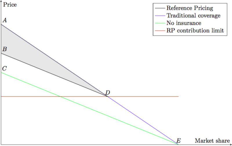
The intuition behind this model is shown in Figure 4. The green line shows demand without insurance coverage, and thus no resulting moral hazard. Introducing insurance coverage shifts demand up to the blue line. The resulting moral hazard under traditional coverage with some coinsurance is given by the “ACE” triangle. Demand under reference pricing is given by the black line and the corresponding moral hazard is given by the much smaller “BCED” area. The non-linear cost-sharing design of the reference pricing program reduces moral hazard by shifting demand away from providers priced above the reference price (“ABD” triangle).

Figure 4.

Moral Hazard Graphical Representation

5.2 Estimation

To estimate consumer choices, we use a control function method to address the endogeneity of OOP_ij in our model. The control function approach was originally proposed by Hausman (1978) and Heckman (1978). Petrin & Train (2010) illustrate that the control function approach is a useful alternative to the commonly used BLP approach (Berry et al., 1995), and these two approaches provide very similar results. In our context, equation 2 is not identified due to the fact that OOP_ij is not independent of ε_ij.

The control function approach posits that OOP_ij can be written as a function of all exogenous variables in δ_ij and an instrument (z_ij). Formally

$${\mathit{\text{OOP}}}_{\mathit{\text{ij}}}(p_j)=W({\mathit{\text{quality}}}_j,{\mathit{\text{distance}}}_{\mathit{\text{ij}}},{\mathit{\text{HOPD}}}_j,z_{\mathit{\text{ij}}};\gamma )+{\mu }_{\mathit{\text{ij}}}$$

The intuition underlying the control function is that when adding the auxiliary variable (μ_ij) to the systematic part of the utility function, the remaining error will be independent of OOP_ij. To get μ_ij, we use patient exposure to the reference pricing program as an instrument for expected out-of-pocket spending at each provider j. That is, we instrument for OOP_ij with a CalPERS_i × post_t × HOPD_j dummy, which is the unit at which the reference pricing program impacts OOP_ij. The identification of this model comes from the exogenous change in OOP_ij(p_j) that is caused by the reference pricing program. Following implementation of reference pricing, the expected out-of-pocket costs for CalPERS patients to visit high-priced HOPDs increases dramatically. We use this exogenous variation in cost-sharing to estimate changes in consumer demand.

Assuming that error terms are independent and identically distributed (iid) and follow a Generalized Extreme Value (GEV) Type I distribution, the predicted choice probabilities are estimated as

$$P_{\mathit{\text{ij}}}=\frac{\text{exp}({\delta }_{\mathit{\text{ij}}})}{{\sum }_{k=1}^K\text{exp}({\delta }_{\mathit{\text{ik}}})}$$ (6)

In δ_ij, we include the quality, distance, cost-sharing measures from equation 2. We also include an indicator for HOPD providers. We operationalize provider quality as the the z-score of the provider’s rate of clinical complications related to colonoscopy relative to other providers in a given HRR. These procedural complications are the same used in the reduced form regressions above. We define distance as the distance between the patient’s zip code and the provider’s zip code. We measure cost-sharing as the expected cost-sharing for each provider in a patient’s choice set based on the patient’s deductible status, the provider’s price, the provider type (e.g. ASC or HOPD), and whether the patient is currently subject to reference pricing. We also further include a full set of interactions between the CalPERS dummy and product attributes to account for heterogeneous preferences between the two patient populations.

5.2.1 Choices Probabilities and Cost Savings

Using the choice estimation parameters, we simulate the post-period choice probabilities for CalPERS patients under both traditional insurance coverage i.e. deductibles and coinsurance) and reference pricing. We denote the choice probabilities under reference pricing as $P_{\mathit{\text{ij}}}^{\mathit{\text{RP}}}$ and the choice probabilities under traditional coverage as $P_{\mathit{\text{ij}}}^{\mathit{\text{TC}}}$. We then aggregate these choices probabilities to get the difference in each provider’s market share under reference pricing and traditional insurance coverage:

$$\mathrm{\Delta }{S}_j=S_j^{\mathit{\text{RP}}}-S_j^{\mathit{\text{TC}}}$$ (7)

The difference in the market shares gives the changes in consumer demand at the provider level. For a given provider j with price p_j, this expression gives the differences in demand for all CalPERS consumers before and after the implementation of the reference pricing program. We then convert ΔS_j to a change in spending by multiplying it by the provider’s price, p_j:

$$\mathrm{\Delta }{\mathit{\text{Spending}}}_j=\mathrm{\Delta }{S}_j{p}_j.$$ (8)

5.2.2 Aggregated Direct Elasticity (ADE) of OOP

Because the identification of the changes in consumer demand are driven by changes in out-of-pocket prices, we can also use the same model to estimate own-price elasticities. The most important provider characteristic change is the change in out-of-pocket prices caused by the reference pricing program. Following Ben-Akiva & Lerman (1985), we define the Aggregated Direct Elasticity (ADE) of OOP as the effect on the share of consumers in market m choosing provider j when there’s an incremental change in OOP.

$${\mathit{\text{ADE}}}_m(j)=\frac{\eta }{{\sum }_{i=1}^{N_m}{P}_{\mathit{\text{ij}}}}\sum _{i=1}^{N_m}(1-P_{\mathit{\text{ij}}})P_{\mathit{\text{ij}}}{\mathit{\text{OOP}}}_{\mathit{\text{ij}}}$$

where N_m is the total number of Anthem and CalPERs consumers in market m and P_ij denotes the fitted choice probabilities. We compute the ADE for all providers in the choices set.

5.2.3 Consumer Welfare

For each CalPERS consumer in the post period, their expected utility difference between traditional coverage and reference pricing can be expressed as

$$E(\mathit{\text{Max}}{U}_i^{\mathit{\text{RP}}})-E(\mathit{\text{Max}}{U}_i^{\mathit{\text{TC}}})=\mathit{\text{ln}}(\sum _{k=1}^K\text{exp}({\delta }_{\mathit{\text{ik}}}^{\mathit{\text{RP}}}))-\mathit{\text{ln}}(\sum _{k=1}^K\text{exp}({\delta }_{\mathit{\text{ik}}}^{\mathit{\text{TC}}})).$$ (9)

Under the assumption that there are no changes in the marginal utility of money, we can compute the compensating variation (or changes in consumer surplus in dollars) by normalizing the above expression by the OOP coefficient:

$$\mathrm{\Delta }{\mathit{\text{ConsumerSurplus}}}_i=\frac{1}{-\eta }(\mathit{\text{ln}}(\sum _{k=1}^K\text{exp}({\delta }_{\mathit{\text{ik}}}^{\mathit{\text{RP}}}))-\mathit{\text{ln}}(\sum _{k=1}^K\text{exp}({\delta }_{\mathit{\text{ik}}}^{\mathit{\text{TC}}}))).$$ (10)

5.3 Construction of Choice Sets

To construct the choice sets of providers available to each patient, we use all providers located within the same Hospital Referral Region (HRR) of the patient’s zip code. Alternative choice sets consisting of all providers in each patient’s hospital service area (HSA) yielded similar results. We include the full sample of the CalPERS and the non-CalPERS population. But patients who selected a hospital outside the HRR of her home address, and out-of-network provider or providers with fewer than 5 observations in any year are excluded from this analysis. We also exclude patients in HRRs with fewer than 5 providers for colonoscopy. On average, each patient in our final study sample has approximately 41 providers in their choice set, although there is substantial variation in the number of available providers. Patients located in the Los Angeles and San Francisco regions have an average of 97 providers while those in the more rural areas of California have an average of 5 available providers.

5.4 Results

Table 9 presents the demand model results. The first column presents the results without any corrections for the correlation between OOP and omitted provider attributes. The results clearly contradicts the expectation of downward sloping demand curve as the endogeneity of OOP_ij(p_j) biases the estimates upward. The second and third columns apply the control function approach by adding the auxiliary variable (μ_ij) to utility function. The price coefficients are corrected to the expected direction and are significantly negative. While the coefficients are not directly interpretable, their signs and magnitudes highlight how different provider attributes change consumer choices. In column 2, all of the provider attributes enter with expected signs. Columns 3 further presents whether the Anthem population’s tastes for these provider attributes differ from that of the CalPERS population. Our results suggest that CalPERS patients are overall more likely to choose a HOPD provider. They are also more likely to choose a provider with a lower relative complication score. We find little difference in their tastes for distance between the patient and the provider.

Table 9.

Choice Regressions

	(1) Uncorrected	(2) With CF	(3) With CF
OOP	0.078*** (0.001)	−0.119*** (0.012)	−0.166*** (0.014)
quality	0.543*** (0.015)	0.387*** (0.018)	0.327*** (0.019)
quality × CalPERS			0.223*** (0.045)
distance	−0.162*** (0.001)	−0.165*** (0.001)	−0.167*** (0.001)
distance × CalPERS			0.019*** (0.002)
HOPD	−1.228*** (0.010)	−0.570*** (0.040)	−0.432*** (0.045)
HOPD × CalPERS			0.309*** (0.038)
Observations	4,004,966	4,004,966	4,004,966

Standard errors in parentheses, OOP is measured in hundreds

^***p<0.01,

^**p<0.05,

^*p<0.1

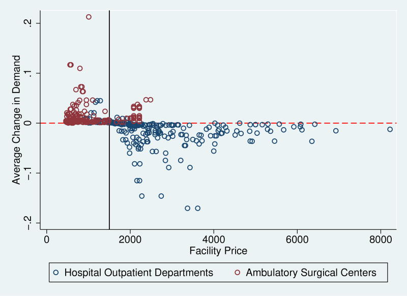
Figure 5 plots the average changes in the choice probabilities (or market share) for each provider from equation 7 against provider prices. The blue points show changes in demand for the HOPDs while the red points show the demand changes for ASCs. For HOPDs, the figure shows an overall reduction in demand for providers with prices above the $1,500 reference price. Moreover, there is an overall decreasing relationship between demand changes and provider prices. For HOPDs whose prices between $1,500–$4,000, compared to the expected demand in the absence of the reference pricing program, the more expensive providers see larger reductions in demand than the less expensive providers. However, for HOPDs with prices above $4,000, there is a much smaller change in demand, regardless of provider prices. In contrast, there is an increase in demand for ASCs with prices both above and below the $1,500 reference price

Figure 5.

Demand Changes

This figure plots the change in demand for each provider, ΔP_j from equation 7, against provider prices.

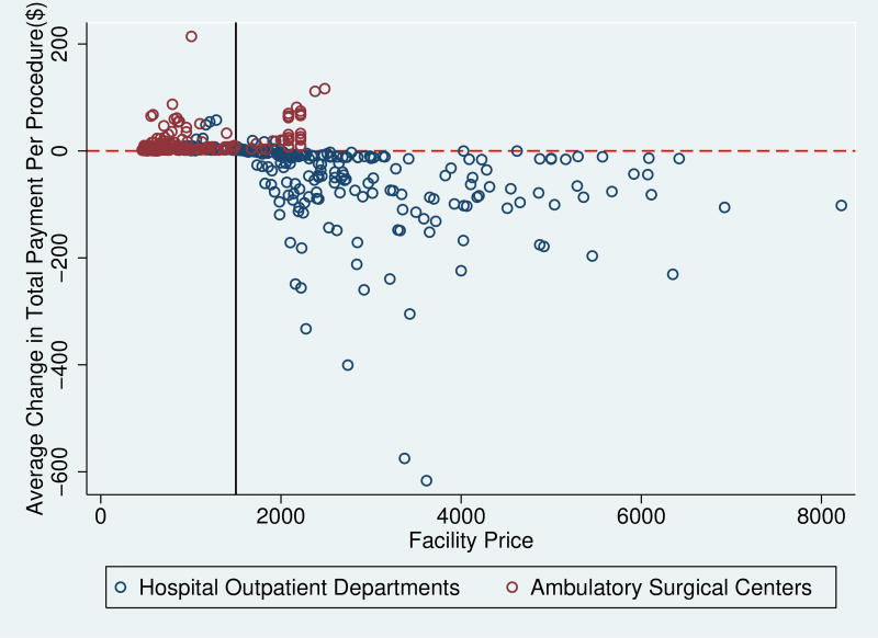
Figure 6 plots the changes in spendings from equation 8 against provider prices. The blue points show changes in spendings for HOPDs with price p_j multiplied by ΔS_j. The red points show the same changes in spendings for ASCs. This figure shows the greatest spending reduction is from HOPDs with prices between $3,000–$4,000. We observe little change in spending for ASCs and for HOPDs that have prices below $2,000.

Figure 6.

Spending Changes

This figure plots the average change in spending at each provider, from equation 8, against provider prices. In this figure, the demand changes from Figure 5 are multiplied by provider prices.

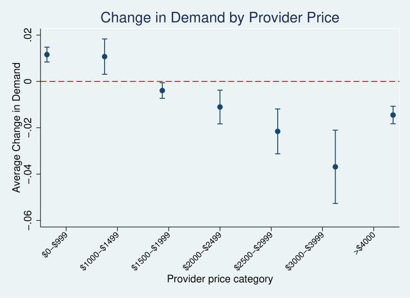
To more formally show the difference in the both demand and spendings, we regress the changes in choice probability and total payment on a dummy for CalPERS vs. Anthem enrollment. We estimate these regressions separately for provider price categories to separately identify the relationship between provider prices and changes in demand and spendings. Figure 7 plots the regression coefficients for changes in demand. We find minimal changes in demand for providers with prices below $3,000. However, for providers with prices between $3,000–$4,000 and above $4,000, we find 3.7 and 1.4 percentage point reductions in demand among CalPERs patients after the implementation of reference pricing. For the upper two price categories, the mean baseline choice probabilities are 5.0% and 1.5%. Thus, our results imply that the reference pricing program leads to an approximately 74% and 93% decrease in demand for these expensive providers. As shown in Figures 5–8, we find little evidence of behavior change around the reference price.

Figure 7.

Demand Change Regressions

This figure plots coefficients from a regression of changes in provider demand (ΔP_j) against a dummy for CalPERS vs. Anthem enrollment.

Figure 8.

Spending Regressions

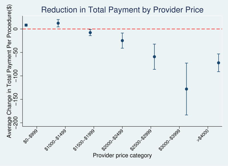
This figure plots coefficients from a regression of changes in spending at each provider against a dummy for CalPERS vs. Anthem enrollment.

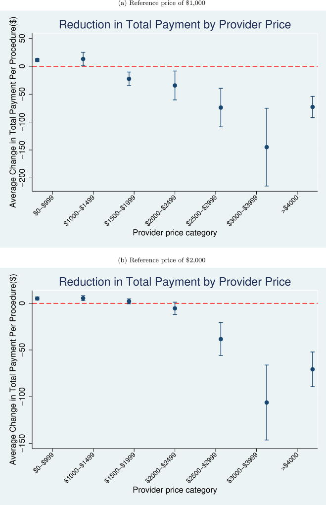
Figure 8 plots similar regression coefficients for changes in total payment. Between $2,000 and $4,000, we find modest reductions in total spending. These reductions range from a $24.7 reduction for prices between $2,000–$2,500, an $59.2 reduction for prices between $2,500–$3,000, and a $128.0 reduction for prices between $3,000 and $4,000. However, we find a smaller, $72.1, reduction for prices above $4,000. For the CalPERS population, we sum ΔPr_ij * P_j across all alternatives in one’s choice set and find an average spending reduction of $218.8 per procedure. This result is similar to the reduced form mean effects discussed above and also the $199 reduction in medical spending reported in Robinson et al. (2015a). However, the substantially larger reduction in spending for providers with prices above $2,500 suggests that most of the effect comes from reductions in demand for these providers. The overall similarity between the results from the reduced form, where we only consider changes in prices, and structural, where we include changes in other provider attributes, models suggests that there is little relationship between provider price and non-price attributes.

Table 10 presents the estimated ADE by provider price category. These elasticities range from positive −0.38 for providers with prices below $1,000 to −1.93 for providers with prices above $4,000. The increasing elasticity with provider prices both follows traditional consumer demand theory and suggests that at high price levels, patients become increasingly sensitive to out-of-pocket spending. The average ADE of all providers in our sample is −0.70. We also calculate the total change in consumer surplus as in equation 10. We find an average decrease in consumer surplus of $94.3 for the CalPERS population after the implementation of the reference pricing program.

Table 10.

Aggregated Direct Elasticity (ADE) of OOP

Provider price	(1) <$1,000	(2) $1,000–$1,500	(3) $1,500–$2,000	(4) $2,000–$2,500	(5) $2,500–$3,000	(6) $3,000–$4,000	(7) >$4,000
ADE (SD)	−0.382 (0.117)	−0.624 (0.168)	−0.782 (0.207)	−0.893 (0.267)	−1.041 (0.309)	−1.181 (0.381)	−1.934 (0.293)

Standard deviations in parentheses.

These elasticity results are higher than the price elasticity results that have traditionally been reported in the literature. A key distinction between these elasticities and the previously reported is that our elasticities represent the change in demand for a given provider given that provider’s price, conditional on receiving care. We do not measure the sensitivity to receiving or not receiving care (the extensive margin) with respect to price. Thus, our elasticities should be thought of as measuring sensitivity to price shopping (the intensive margin). Our own-price elasticities are smaller than the elasticities of −2.3 to −4.2 for California hospitals reported in Gaynor & Vogt (2003). One potential reason is that the Gaynor elasticities cover price sensitivity for all hospital services while we focus on a single service, colonoscopy. Our elasticity estimates are also similar to the upper bound of the results in Goldman et al. (2007), which finds elasticity with respect to spending of −0.2 to −0.6 for pharmaceuticals. One potential reason why our own-price elasticities and the overall spending elasticities in Goldman et al. (2007) are similar is that many pharmaceuticals have multiple close substitutes. Thus it is likely that a larger share of spending reductions occur through substitution between providers rather than changes in utilization for pharmaceuticals than for other health care services.

6 Counterfactuals

We next use the structural parameters from our choice model to investigate the impact of two counterfactuals–changing the reference price limit and implementing altogether different insurance benefit designs. First, we estimate the effects of altering the reference pricing program with two different reference price limits: $1,000 and $2,000. Second, we estimate the effects of two alternative benefit designs–no insurance and a high-deductible health plan. For both, we use the same model coefficients from Table 9 but change the patient cost-sharing schedule based on the each alternative scenario.

6.1 Alternative Reference Prices

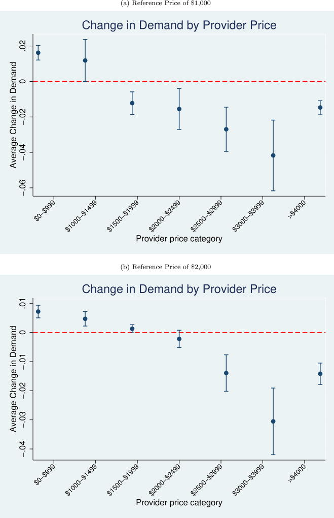
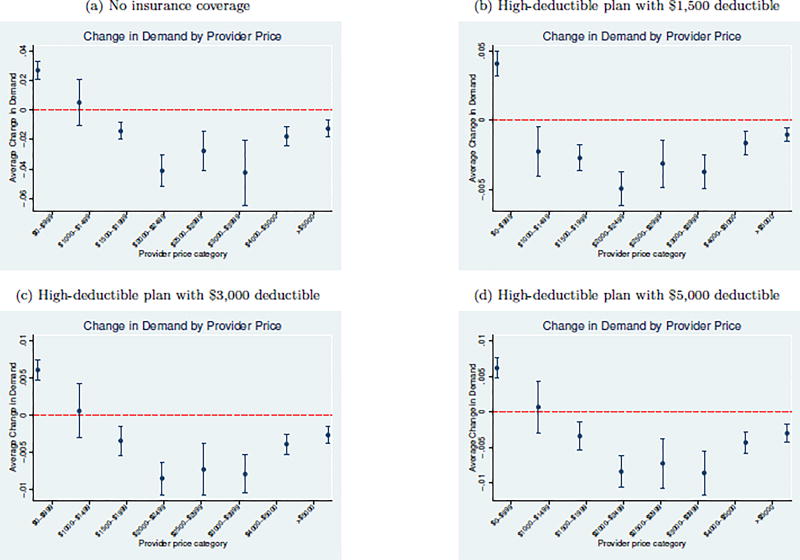
Figure 10 plots the regression coefficients for estimated changes in demand under each scenario. The top figure presents the changes in demand for the $1,000 reference price while the bottom figure plots the estimated changes in demand under a $2,000 reference price. Under both counterfactual scenarios, we find minimal changes in demand for providers with prices below $2,500. However, for providers with prices between $3,000–$4,000 and above $4,000, we find an approximately 4.17 and 1.46 percentage point reduction in demand if the reference price limit were set at $1,000. The corresponding figures are 3.05 and 1.42 if the reference price limit were set at $2,000.

Figure 10.

Counterfactual Total Spending Change from Alternative Reference Price

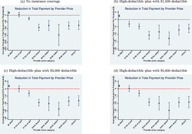
Similarly, Figure 10 plots regression coefficients for changes in spending under the two counterfactual scenarios. If the reference price limit were set at $1,000 per colonoscopy, we find reductions in spending for providers whose price is above $1,500. Specifically, the spending reduction is $22.5 for prices between $1,500–$2,000, $34.3 for prices between $2,000–$2,500, $73.9 for prices between $2,500–$3,000, $144.9 for prices between $3,000 and $4,000, and $72.9 for prices above $4,000. If the reference price were set at $2,000, we find modest reduction in spending for providers in all the above price categories except for the $1,500–$2,000 group. The spending reductions are $5.4, $38.4, $106.3 and $70.7 for prices between $2,000–$2,500, $2,500–$3,000, $3,000-$4,000 and above $4,000, respectively.

Across both scenarios, we estimate an average reduction in spending of $281.4 under the $1,000 reference price and $157.4 under the $2,000 reference price. Compared to the $218.8 estimate from the actual $1,500 reference price, the counterfactual estimates are similar. The intuition for this similarity is largely due to the heterogeneous change in consumer demand. Near the reference price, consumers are relatively insensitive to provider prices. Under all three reference price scenarios, not until the $2,000 price point does consumer demand change modestly and not until the $2,500 price point does it change substantially. The similarity of the estimated spending suggests that near the $1,500 mark, the choice of the specific reference price does not have a large effect on patient demand. However, there are differences in how much of the reference pricing program’s savings are due to changing demand for expensive providers versus shifting costs to consumers. We estimate that average consumer surplus would decrease by $141.7 and $54.6 if the reference price limit were set at $1,000 or $2,000, respectively.

6.2 Alternative Insurance Designs

We next use the model parameters to estimate the effects of two alternative benefit designs–no insurance coverage and a high-deductible plan with a deductible of $1,500, $3,000 and $5,000. For each counterfactual, we follow the model in Section 5.1 and apply the parameters in Table 9 column (3). For brevity, we present the full figures in Appendix Figures B.1 and B.2. Our results imply that moving from uninsured to traditional insurance coverage leads to a $407.5 increase in total payment per colonoscopy procedure and an average increase in consumer surplus of $751.6. Thus, reference pricing reduces the increased spending of insurance coverage, intensive-margin moral hazard, per colonoscopy by approximately 53.7% at the expenses of reducing the consumer surplus by only 12.5%.

On the other hand, compared to traditional insurance coverage, we estimate that a $1,500 deductible, a $3,000 deductible, and a $5,000 deductible would lead to a reduction in spending of $60.5, $91.2, and $93.1, respectively. Thus, the reduction in spending from reference pricing is about two to three times as large as the reduction due to implementing a HDHP. The consumer surplus reductions are $125.9, $140.7, and $141.1 if a deductible of $1,500, $3,000, or $5,000 were implemented. All the counterfactual HDHPs will lead to a greater reduction in consumer welfare but a smaller cost saving.

The differences in cost savings largely stem from differences in patient price sensitivity across the provider price distribution. By definition, HDHP plans only protect consumer’s spending until the deductible is reached. However, this paper’s results show that patients are most price sensitive well above the deductible. In this setting, by providing coverage above the deductible, HDHPs do not protect against spendings at the price ranges in which patients are most likely to shop. In contrast, the similarity between the no-insurance and the reference pricing designs are largely because each design fully exposes patients to the upper tail of prices, which is where patients are the most price-sensitive.

7 Conclusion

Health care prices for the commercially insured population are marked by substantial levels of variation Cooper et al. (2015). Insurer programs that attempt to respond to this variation by shifting demand to low-priced providers have been met with limited success. This paper examines consumer responses to an innovative benefit design implemented by CalPERS for colonoscopy services. The reference pricing program’s non-linear cost-sharing provides explicit incentives for consumers to receive care from less expensive providers. Following similar work, we find that the program increases demand for the low-priced providers and leads to a sizable reduction in the average cost per colonoscopy.

A large source of patients’ existing lack of price responsiveness is due to the presence of generous insurance coverage, which creates excessive medical expenditures. The CalPERS reference pricing is unique in the sense that it targets the type of excessive medical expenditures by incentivizing patients to receive care from less expensive providers. This type of excessive medical expenditures has not been previously studied. To estimate changes in medical spending and consumer welfare, we use the exogenous change in consumer cost-sharing induced by the program to estimate aggregated direct elasticities that range from −0.38 to −1.93. The program leads to an approximately $218.8 decrease in spending that occurs along the intensive margin of provider prices and a $94.3 decrease in consumer welfare. The former is approximately 53.7% of the overall spending increase of insurance coverage while the latter is only 12.5% of the average increase in consumer surplus caused by insurance coverage. Our counterfactuals suggest that near the chosen reference price of $1,500 mark, the choice of the specific reference price does not have a large effect on patient demand or consumer surplus. However, if a deductible of $1,500, $3,000 and $5,000 were implemented, the cost savings would be much smaller while the consumer welfare reduction would be much larger.

One limitation of this paper is that we do not examine colonoscopy utilization decisions. We do not examine the extensive margin decision of whether or not to receive a colonoscopy or the alternative intensive margin of the number of colonoscopies. Both dimensions are more commonly studied than the price margin that we consider in this paper. We find a sizable increase in patient cost-sharing for colonoscopies and so we may be concerned that some patients elect to not receive the procedure. Because colonoscopies are an especially effective form of cancer screening, reducing utilization may have important implications for overall patient health and welfare. Future studies should examine if the CalPERS reference pricing program has unintended consequences on the use of colonoscopies or patient health.

One limitation to the generalizability of our results is that we examine a single service using data from a single firm. CalPERS may have implemented reference pricing based on prior knowledge that the program would work better for the CalPERS population than it would for other populations (Allcott, 2015). However, the level of price variation observed for colonoscopies in our data is common across the health care landscape. Thus, the results of this study suggest that for other services with easily substitutable providers, reference pricing programs may be useful mechanisms to encourage patients to shop for care.

Figure 9.

Counterfactual Demand Change Regressions from Alternative Reference Price

Table 8.

Effect of Patient Cost-Sharing on Patient Choice of Provider

	Full Sample			Restricted Markets
	(1) ln(price)	(2) ln(price)	(3) ln(price)	(4) ln(price)	(5) ln(price)	(6) ln(price)
ln(patient+1)	−0.597*** (0.183)	−0.565*** (0.165)	−0.454*** (0.120)	−0.769*** (0.120)	−0.780*** (0.105)	−0.784*** (0.129)
Observations	320,826	320,826	320,826	192,705	192,705	192,705
First stage F stat	195.84	226.76	267.81	63.67	67.93	64.72
Fixed Effects		HRR	HRR × year		HRR	HRR × year

This table presents the 2SLS results where patient out-of-pocket spending is instrumented for using exposure to the reference pricing program. The dependent variable is the log of the total colonoscopy cost as the dependent variable. All columns include controls for patient demographics (age, gender, Charlson risk score), the primary colonoscopy procedure code, and month. Columns 2 and 5 add patient HRR fixed effects while columns 3 and 6 add year by patient HRR interactions. Robust standard errors clustered at the provider level are in parentheses.

^***p<0.01,

^**p<0.05,

^*p<0.1.

A Reduced Form Robustness Tests

Table A.1.

Yearly Changes in Colonoscopy Prices

	(1) ln(price)	(2) ln(price)	(3) ln(price)
CalPERS × 2009	0.0199 (0.0231)	0.0242 (0.0189)	0.0251 (0.0215)
CalPERS × 2010	0.0308 (0.0199)	0.0402** (0.0173)	0.0364* (0.0205)
CalPERS × 2012	−0.124*** (0.0268)	−0.116*** (0.0274)	−0.104*** (0.0266)
CalPERS × 2013	−0.107*** (0.0194)	−0.110*** (0.0191)	−0.0960*** (0.0181)
CalPERS	0.174*** (0.0444)	0.0997*** (0.0241)	0.0948*** (0.0234)
2009	−0.107*** (0.0175)	−0.118*** (0.0164)	0.216*** (0.00563)
2010	−0.0671*** (0.0125)	−0.0768*** (0.0108)	0.104*** (0.00588)
2012	0.107*** (0.0255)	0.111*** (0.0269)	0.221*** (0.0115)
2013	0.140*** (0.0266)	0.150*** (0.0293)	0.223*** (0.00753)
Observations	320,826	320,826	320,826
R2	0.028	0.141	0.148
Mean CalPERS 2011 price	1,716	1,716	1,716
Fixed Effects		HRR	HRR × year

This table presents the difference-in-differences results from equation 1 and uses the log of the total colonoscopy cost as the dependent variable. All columns include controls for patient demographics (age, gender, Charlson risk score), the primary colonoscopy procedure code, and month. Column 2 adds patient HRR fixed effects and column 3 adds year by patient HRR interactions. Robust standard errors clustered at the provider level are in parentheses.

^***p<0.01,

^**p<0.05,

^*p<0.1.

Table A.2.

Yearly Changes in Patient Cost Sharing

	(1) ln(patient+1)	(2) ln(patient+1)	(3) ln(patient+1)
CalPERS × 2009	0.0614** (0.0289)	0.0715** (0.0302)	0.0769** (0.0333)
CalPERS × 2010	0.103*** (0.0281)	0.0995*** (0.0278)	0.0880*** (0.0315)
CalPERS × 2012	0.306*** (0.0558)	0.321*** (0.0558)	0.343*** (0.0507)
CalPERS × 2013	0.248*** (0.0543)	0.267*** (0.0549)	0.296*** (0.0561)
CalPERS	−0.00497 (0.0281)	0.0210 (0.0208)	0.0119 (0.0209)
2009	0.0177 (0.0442)	0.0299 (0.0448)	−0.0648 (0.0659)
2010	−0.0254 (0.0216)	−0.0132 (0.0214)	−0.172*** (0.0430)
2012	0.0836* (0.0461)	0.0735 (0.0456)	0.123** (0.0490)
2013	0.0831 (0.0513)	0.0658 (0.0488)	0.0971*** (0.0119)
Observations	320,826	320,826	320,826
R2	0.771	0.775	0.776
Mean CalPERS 2011 cost-share	205	205	205
Fixed Effects		HRR	HRR × year

This table presents the difference-in-differences results from equation 1 and uses the log of patient spending as the dependent variable. All columns include controls for patient demographics (age, gender, Charlson risk score), the primary colonoscopy procedure code, and month. Column 2 adds patient HRR fixed effects and column 3 adds year by patient HRR interactions. Robust standard errors clustered at the provider level are in parentheses.

^***p<0.01,

^**p<0.05,

^*p<0.1.

Table A.3.

Yearly Changes in Employer and Insurer Spending

	(1) ln(paid+1)	(2) ln(paid+1)	(3) ln(paid+1)
CalPERS × 2009	0.125** (0.0467)	0.125*** (0.0438)	0.105** (0.0481)
CalPERS × 2010	0.124*** (0.0413)	0.145*** (0.0397)	0.121*** (0.0425)
CalPERS × 2012	−0.0861** (0.0403)	−0.0924** (0.0384)	−0.0720* (0.0399)
CalPERS × 2013	−0.167** (0.0667)	−0.194*** (0.0687)	−0.167** (0.0676)
CalPERS	0.716*** (0.0887)	0.581*** (0.0901)	0.582*** (0.0868)
2009	0.0349 (0.0398)	0.00510 (0.0396)	0.918*** (0.0298)
2010	0.0135 (0.0290)	−0.0145 (0.0282)	0.561*** (0.0211)
2012	0.119*** (0.0354)	0.137*** (0.0364)	0.425*** (0.0180)
2013	0.220*** (0.0454)	0.254*** (0.0498)	0.440*** (0.0255)
Observations	320,826	320,826	320,826
R2	0.113	0.154	0.156
Mean CalPERS 2011 paid amount	1,511	1,511	1,511
Fixed Effects		HRR	HRR × year

This table presents the difference-in-differences results from equation 1 and uses the log of employer and insurer spending on colonoscopy services (i.e. allowed amount - patient cost-sharing) as the dependent variable. All columns include controls for patient demographics (age, gender, Charlson risk score), the primary colonoscopy procedure code, and month. Column 2 adds patient HRR fixed effects and column 3 adds year by patient HRR interactions. Robust standard errors clustered at the provider level are in parentheses.

^***p<0.01,

^**p<0.05,

^*p<0.1.

Table A.4.

Yearly Changes in Patient Choice of Colonoscopy Provider

	HOPD
	(1) covered	(2) covered	(3) covered
CalPERS × 2009	0.00766 (0.0124)	0.00570 (0.0109)	0.0165 (0.0107)
CalPERS × 2010	0.0166 (0.0103)	0.0120 (0.00772)	0.0123 (0.0101)
CalPERS × 2012	0.0697*** (0.0106)	0.0643*** (0.0116)	0.0616*** (0.0112)
CalPERS × 2013	0.103*** (0.0168)	0.104*** (0.0171)	0.0953*** (0.0154)
CalPERS	−0.0727*** (0.0230)	−0.0329** (0.0130)	−0.0326** (0.0134)
2009	0.0150 (0.0106)	0.0225** (0.0106)	−0.154*** (0.00353)
2010	0.00385 (0.00713)	0.0108* (0.00610)	−0.0920*** (0.00328)
2012	−0.00702 (0.0110)	−0.00723 (0.0117)	−0.104*** (0.00787)
2013	−0.0211 (0.0179)	−0.0227 (0.0189)	−0.0909*** (0.00366)
Observations	320,826	320,826	320,826
Mean CalPERS 2011 share	0.70	0.70	0.70
Fixed Effects		HRR	HRR × year

This table presents the difference-in-differences results from equation 1 and uses the probability of choosing either an ASC or an HOPD with a price below $1,500 as the dependent variable. All columns include controls for patient demographics (age, gender, Charlson risk score), the primary colonoscopy procedure code, and month. Column 2 adds patient HRR fixed effects and column 3 adds year by patient HRR interactions. Robust standard errors clustered at the provider level are in parentheses.

^***p<0.01,

^**p<0.05,

^*p<0.1.

Table A.5.

Yearly Changes in Procedural Complications

	(1) complication	(2) complication	(3) complication
CalPERS × 2009	0.00112 (0.00211)	0.00109 (0.00209)	−0.0000290 (0.00198)
CalPERS × 2010	0.00275 (0.00303)	0.00273 (0.00304)	0.00218 (0.00306)
CalPERS × 2012	−0.00131 (0.00211)	−0.00156 (0.00211)	−0.000841 (0.00219)
CalPERS × 2013	−0.000644 (0.00349)	−0.000895 (0.00343)	−0.000436 (0.00358)
CalPERS	−0.00104 (0.00229)	−0.000196 (0.00211)	−0.0000463 (0.00217)
2009	−0.00268*** (0.000710)	−0.00267*** (0.000716)	0.00206** (0.000783)
2010	−0.000917 (0.000937)	−0.000937 (0.000954)	0.00372*** (0.000895)
2012	−0.000285 (0.000782)	−0.000226 (0.000776)	0.00239** (0.00109)
2013	−0.00189* (0.000983)	−0.00186* (0.000965)	0.00690*** (0.00118)
Observations	320,826	320,826	320,826
R2	0.021	0.021	0.022
Mean CalPERS 2011 complication rate	0.020	0.020	0.020
Fixed Effects		HRR	HRR × year

This table presents the difference-in-differences results from equation 1 and uses the probability of receiving a procedural complication related to colonoscopy as the dependent variable. All columns include controls for patient demographics (age, gender, Charlson risk score), the primary colonoscopy procedure code, and month. Column 2 adds patient HRR fixed effects and column 3 adds year by patient HRR interactions. Robust standard errors clustered at the provider level are in parentheses.

^***p<0.01,

^**p<0.05,

^*p<0.1.

Table A.6.

Yearly Changes in Distance Travelled

	(1) ln(distance+1)	(2) ln(distance+1)	(3) ln(distance+1)
CalPERS × 2009	−0.0206 (0.0310)	−0.0215 (0.0234)	−0.0153 (0.0236)
CalPERS × 2010	−0.0297 (0.0293)	−0.0134 (0.0233)	−0.0155 (0.0240)
CalPERS × 2012	0.00356 (0.0293)	−0.0111 (0.0274)	−0.0102 (0.0288)
CalPERS × 2013	−0.0514 (0.0402)	−0.0630 (0.0402)	−0.0441 (0.0361)
CalPERS	0.0588 (0.0920)	−0.0225 (0.0331)	−0.0264 (0.0336)
2009	0.0233 (0.0245)	−0.00589 (0.0169)	0.0829*** (0.00955)
2010	0.0485** (0.0207)	0.0168 (0.0126)	0.0556*** (0.00774)
2012	−0.00875 (0.0112)	0.00278 (0.0103)	0.343*** (0.0132)
2013	−0.000598 (0.0252)	0.0222 (0.0227)	0.778*** (0.00893)
Observations	320,826	320,826	320,826
R2	0.004	0.130	0.133
Mean CalPERS 2011 distance	33	33	33
Fixed Effects		HRR	HRR × year

This table presents the difference-in-differences results from equation 1 and uses the distance between the patient’s zip code and the provider’s zip code as the dependent variable. All columns include controls for patient demographics (age, gender, Charlson risk score), the primary colonoscopy procedure code, and month. Column 2 adds patient HRR fixed effects and column 3 adds year by patient HRR interactions. Robust standard errors clustered at the provider level are in parentheses.

^***p<0.01,

^**p<0.05,

^*p<0.1.

Figure A.1.

Quarterly Differences in Outcomes

Figure A.2.

Monthly Differences in Outcomes

B Alternative Benefit Designs

Figure B.1.

Counterfactual Demand Change Regressions from Alternative Benefit Design

Figure B.2.

Counterfactual Spending Regressions from Alternative Benefit Design

References

- Allcott Hunt. Site Selection Bias in Program Evaluation. The Quarterly Journal of Economics. 2015;130(3):1117–1165. [Google Scholar]
- Aouad Marion, Brown Timothy T, Whaley Christopher. Quantile Treatment Effects of Reference Pricing. Tech. rept. University of California; Berkeley: 2017a. [Google Scholar]
- Aouad Marion, Brown Timothy, Whaley Christopher. Reference Pricing - The Case of Screening Colonoscopies. Tech. rept. University of California; Berkeley: 2017b. 00000. [DOI] [PMC free article] [PubMed] [Google Scholar]
- Arrow Kenneth J. Uncertainty and the Welfare Economics of Medical Care. The American Economic Review. 1963;53(5):941–973. [Google Scholar]
- Baicker Katherine, Goldman Dana. Patient Cost-Sharing and Healthcare Spending Growth. Journal of Economic Perspectives. 2011;25(2):47–68. doi: 10.1257/jep.25.2.47. [DOI] [PubMed] [Google Scholar]
- Ben-Akiva Moshe E, Lerman Steven R. Discrete choice analysis: theory and application to travel demand. Vol. 9. MIT press; 1985. [Google Scholar]
- Berry Steven, Levinsohn James, Pakes Ariel. Automobile prices in market equilibrium. Econometrica: Journal of the Econometric Society. 1995:841–890. [Google Scholar]
- Brot-Goldberg Zarek C, Chandra Amitabh, Handel Benjamin R, Kolstad Jonathan T. Working Paper 21632. National Bureau of Economic Research; 2015. Oct. What Does a Deductible Do? The Impact of Cost-Sharing on Health Care Prices, Quantities, and Spending Dynamics. [Google Scholar]
- Charlson ME, Pompei P, Ales KL, MacKenzie CR. A New Method of Classifying Prognostic Comorbidity in Longitudinal Studies: Development and Validation. Journal of Chronic Diseases. 1987;40(5):373–383. doi: 10.1016/0021-9681(87)90171-8. [DOI] [PubMed] [Google Scholar]
- Cooper Zack, Craig Stuart V, Gaynor Martin, Reenen John Van. Working Paper 21815. National Bureau of Economic Research; 2015. Dec. The Price Ain’t Right? Hospital Prices and Health Spending on the Privately Insured. [Google Scholar]
- Cutler David M, Zeckhauser Richard J. Chapter 11 The anatomy of health insurance. In: Anthony J Culyer, Joseph P., editors. Handbook of Health Economics. Part A. Vol. 1. Newhouse: Elsevier; 2000. pp. 563–643. of: [Google Scholar]
- Einav Liran, Finkelstein Amy, Ryan Stephen P, Schrimpf Paul, Cullen Mark R. Selection on Moral Hazard in Health Insurance. American Economic Review. 2013;103(1):178–219. doi: 10.1257/aer.103.1.178. [DOI] [PMC free article] [PubMed] [Google Scholar]
- Einav Liran, Finkelstein Amy, Schrimpf Paul. The Response of Drug Expenditure to Nonlinear Contract Design: Evidence from Medicare Part D. The Quarterly Journal of Economics. 2015;130(2):841–899. doi: 10.1093/qje/qjv005. [DOI] [PMC free article] [PubMed] [Google Scholar]
- Feldman Roger, Dowd Bryan. A New Estimate of the Welfare Loss of Excess Health Insurance. The American Economic Review. 1991;81(1):297–301. [PubMed] [Google Scholar]
- Feldstein Martin S. The Welfare Loss of Excess Health Insurance. Journal of Political Economy. 1973;81(2, Part 1):251–280. [Google Scholar]
- Frank Matthew B, Hsu John, Landrum Mary Beth, Chernew Michael E. The Impact of a Tiered Network on Hospital Choice. Health Services Research. 2015;50(5):1628–1648. doi: 10.1111/1475-6773.12291. [DOI] [PMC free article] [PubMed] [Google Scholar]
- Frick Kevin D, Chernew Michael E. Beneficial Moral Hazard and the Theory of the Second Best. Inquiry. 2009;46(2):229–240. doi: 10.5034/inquiryjrnl_46.02.229. [DOI] [PubMed] [Google Scholar]
- Gaynor Martin, Vogt William B. Competition among Hospitals. The RAND Journal of Economics. 2003;34(4):764–785. [PubMed] [Google Scholar]
- Goldman Dana, Joyce Geoffrey, Zheng Yuhui. Prescription Drug Cost Sharing: Associations with Medication and Medical Utilization and Spending and Health. JAMA. 2007;298(1):61–69. doi: 10.1001/jama.298.1.61. [DOI] [PMC free article] [PubMed] [Google Scholar]
- Gruber Jonathan, McKnight Robin. Controlling Health Care Costs through Limited Network Insurance Plans: Evidence from Massachusetts State Employees. American Economic Journal: Economic Policy. 2016;8(2):219–250. 00016. [Google Scholar]
- Hausman Jerry A. Specification tests in econometrics. Econometrica: Journal of the Econometric Society. 1978:1251–1271. [Google Scholar]
- Haviland Amelia M, Eisenberg Matthew D, Mehrotra Ateev, Huckfeldt Peter J, Sood Neeraj. Do Consumer-Directed health plans bend the cost curve over time? Journal of Health Economics. 2016 Mar.46:33–51. doi: 10.1016/j.jhealeco.2016.01.001. [DOI] [PubMed] [Google Scholar]
- Heckman James J. Dummy Endogenous Variables in a Simultaneous Equation System. Econometrica. 1978;46(4):931–959. [Google Scholar]
- Huckfeldt Peter J, Haviland Amelia, Mehrotra Ateev, Wagner Zachary, Sood Neeraj. Working Paper 20927. National Bureau of Economic Research; 2015. Feb. Patient Responses to Incentives in Consumer-Directed Health Plans: Evidence from Pharmaceuticals. [Google Scholar]
- Joyce Geoffrey F, Zissimopoulos Julie, Goldman Dana P. Digesting the doughnut hole. Journal of Health Economics. 2013;32(6):1345–1355. doi: 10.1016/j.jhealeco.2013.04.007. 00009. [DOI] [PMC free article] [PubMed] [Google Scholar]
- Kowalski Amanda E. Working Paper 18108. National Bureau of Economic Research; 2012. May, Estimating the Tradeoff Between Risk Protection and Moral Hazard with a Nonlinear Budget Set Model of Health Insurance. [DOI] [PMC free article] [PubMed] [Google Scholar]
- Manning Willard G, Newhouse Joseph P, Duan Naihua, Keeler Emmett B, Leibowitz Arleen. Health Insurance and the Demand for Medical Care: Evidence from a Randomized Experiment. The American Economic Review. 1987;77(3):251–277. [PubMed] [Google Scholar]
- MedPAC. March 2016 Report to the Congress: Medicare Payment Policy. Tech. rept. Medicare Payment Advisory Commission; 2016. [Google Scholar]
- Pauly Mark V. The Economics of Moral Hazard: Comment. The American Economic Review. 1968;58(3):531–537. [Google Scholar]
- Petrin Amil, Train Kenneth. A control function approach to endogeneity in consumer choice models. Journal of marketing research. 2010;47(1):3–13. [Google Scholar]
- Robinson James C, Brown Timothy T. Increases In Consumer Cost Sharing Redirect Patient Volumes And Reduce Hospital Prices For Orthopedic Surgery. Health Affairs. 2013;32(8):1392–1397. doi: 10.1377/hlthaff.2013.0188. [DOI] [PubMed] [Google Scholar]
- Robinson James C, Brown Timothy T, Whaley Christopher, Finlayson Emily. Association of Reference Payment for Colonoscopy With Consumer Choices, Insurer Spending, and Procedural Complications. JAMA Internal Medicine. 2015a Sept.:1–7. doi: 10.1001/jamainternmed.2015.4588. [DOI] [PMC free article] [PubMed] [Google Scholar]
- Robinson James C, Brown Timothy T, Whaley Christopher, Bozic Kevin J. Consumer Choice Between Hospital-Based and Freestanding Facilities for Arthroscopy. J Bone Joint Surg Am. 2015b;97(18):1473–1481. doi: 10.2106/JBJS.O.00240. [DOI] [PMC free article] [PubMed] [Google Scholar]
- Robinson James C, Brown Timothy, Whaley Christopher. Reference-Based Benefit Design Changes Consumers Choices And Employers Payments For Ambulatory Surgery. Health Affairs. 2015c;34(3):415–422. doi: 10.1377/hlthaff.2014.1198. [DOI] [PMC free article] [PubMed] [Google Scholar]
- Sood Neeraj, Wagner Zachary, Huckfeldt Peter, Haviland Amelia M. Price Shopping in Consumer- Directed Health Plans. Forum for Health Economics and Policy. 2013;16(1) doi: 10.1515/thep-2012-0028. [DOI] [PMC free article] [PubMed] [Google Scholar]