Cumulant expansions for measuring water exchange using diffusion MRI

Abstract

The rate of water exchange across cell membranes is a parameter of biological interest and can be measured by diffusion magnetic resonance imaging (dMRI). In this work, we investigate a stochastic model for the diffusion-and-exchange of water molecules. This model provides a general solution for the temporal evolution of dMRI signal using any type of gradient waveform, thereby generalizing the signal expressions for the Kärger model. Moreover, we also derive a general nth order cumulant expansion of the dMRI signal accounting for water exchange, which has not been explored in earlier studies. Based on this analytical expression, we compute the cumulant expansion for dMRI signals for the special case of single diffusion encoding (SDE) and double diffusion encoding (DDE) sequences. Our results provide a theoretical guideline on optimizing experimental parameters for SDE and DDE sequences, respectively. Moreover, we show that DDE signals are more sensitive to water exchange at short-time scale but provide less attenuation at long-time scale than SDE signals. Our theoretical analysis is also validated using Monte Carlo simulations on synthetic structures.

I. INTRODUCTION

Diffusion magnetic resonance imaging (dMRI) is widely used to probe microstructure of cells and permeability of porous media via the diffusive motion of water molecules.^1–4 A common approach for measuring water exchange using dMRI is to apply Kärger’s model⁵ to fit the dMRI signal measured by the standard Stejskal-Tanner sequence,⁶ here referred to as the single diffusion encoding (SDE) sequence.⁷ In the Kärger model, molecular motion in different tissue compartments is modeled by free diffusion with different diffusion coefficients. Molecules are assumed to have a stationary probability to jump between compartments. This oversimplified assumption ignores the dependence of location on exchange of molecules but can be justified when the exchange is “barrier limited.”^8,9 This means that molecules within each compartment are well mixed, as diffusion is faster than the exchange so that the dependence of exchange on location can be neglected.

Exchange measurements using the Kärger model were originally proposed only for SDE sequences,⁵ but later studies suggested benefits of double diffusion encoding (DDE) sequences.^10,11 Recently, the DDE-based filter exchange imaging (FEXI) technique was proposed to enable in vivo imaging of exchange rates on clinical MRI scanners.¹² The FEXI approach provides an apparent exchange rate (AXR) sensitive to tissue permeability and has been applied to study human brain tissue,¹³ brain tumors,¹⁴ breast cancer,¹⁵ and kidney.¹⁶ However, the AXR can be sensitive to deviations from the idealised DDE experiment arising due to, for example, imaging gradients.¹⁷ Moreover, there are no theoretical guidelines available for selecting the optimal experimental parameters, although some work has been done using numerical optimization techniques.¹⁴ Furthermore, the difference between FEXI and standard SDE and DDE sequences has not been thoroughly analyzed.

To overcome these limitations, we propose a general approach for modeling the dMRI signal in a diffusion-and-exchange system. Our method accepts any type of gradient waveform and is developed based on a stochastic differential equation that provides a probability distribution of the diffusion-and-exchange process of molecules. As a result of this stochastic model, we derive a generalized model to characterize the temporal evolution of dMRI signal under any type of gradient waveform. This general model reduces to the standard Kärger’s model in the special case of SDE sequences. We also derive the cumulant expansion of the dMRI signal for any type of sequence accounting for water exchange. Based on the cumulant expansion, we compare the dMRI signal from SDE and DDE sequences and design the optimal parameters for different sequences under constraints on the maximal b-value and diffusion time. We also derive an explicit expression for the special case of the FEXI sequence. Monte Carlo simulations show excellent agreement with our theoretical results.

II. THEORY

A. Modeling of diffusion-and-exchange processes

Our approach for modeling the dMRI signal due to diffusion and exchange of molecules in a multi-compartment system uses the following stochastic differential equation:

$$d{\mathit{x}}_t=\sigma ({\mathit{x}}_t)d{\mathit{w}}_t,$$ (1)

where ${\mathit{x}}_t\in {\mathbb{R}}^3$ denotes the location of a water molecule and ${\mathit{w}}_t$ represents the standard Wiener process with $d{\mathit{w}}_{t_1}$ and $d{\mathit{w}}_{t_2}$ being independent Gaussian random variables if t₁ ≠ t₂ with covariance given by

$$\mathcal{E}(d{\mathit{w}}_{t}d{\mathit{w}}_t^{\prime })=Idt,$$

where a′ denotes the transpose of a vector a, I denotes the identity matrix of size 3 × 3, and σ(x_t) represents the variance of dx_t. Throughout this paper, boldface small letters, e.g., $\mathit{w}$, a, represent vector-valued variables. We assume that the variance is isotropic, i.e., $\sigma ({\mathit{x}}_t)\in \mathbb{R}$, to simplify notations, though the results of this paper can be extended in a straightforward manner to a more general setting when σ(x_t) is matrix-valued. Thus, the covariance of the increment dx_t is given by $\mathcal{E}(d{\mathit{x}}_{t}d{\mathit{x}}_t^{\prime })={\sigma }^2({\mathit{x}}_t)Idt$. Moreover, the location x_t of a molecule is also characterized by a state $s({\mathit{x}}_t)\in \left\{\mathrm{1,2}\right\}$, which determines the value of σ(x). To simplify notations, we denote s(x_t) by s(t). Moreover, we assume that

$$\sigma {({\mathit{x}}_t)}^2=\left\{\begin{array}{cc}2D_1,\hfill & \text{if\hspace{0.17em}}s(t)=1,\hfill \\ 2D_2,\hfill & \text{if\hspace{0.17em}}s(t)=2,\hfill \end{array}\right.$$

where D₁ ≠ D₂ and they represent the scalar-valued diffusion coefficients for the two compartments, respectively.

An important assumption we have made in all our derivations above is that the diffusivity is constant (time-invariant) at the experimental time scale being used in this work. Such an assumption is well-founded as the apparent diffusion coefficient (ADC) has very pronounced time-dependence only at short time scales and converges to the “bulk” diffusion coefficient D_∞ at long time scales.¹⁸ Recent studies¹⁹ also show very slowly varying or constant diffusivity at long time scale in biological tissue. Since exchange occurs at long time scale, the diffusion coefficient can be assumed to be constant. The two diffusion coefficients, D₁ and D₂, represent the long-time diffusive motion of water molecules in two structures, e.g., intra- and extra-cellular spaces. In situations where the time scale for the exchange is short, restrictions and hindrances induced time-varying diffusivity needs to be considered.^20–22 In this case, a more realistic model, such as the Ornstein-Uhlenbeck model,^23,24 can be used for modeling the two types of diffusive motions. But, we will only focus on Eq. (1) in this paper. Alternatively, a Langevin equation with fluctuating diffusivity was assumed to switch between two constant states.^25,26 Here, we propose a different approach from Refs. ²⁵ and ²⁶ for modeling the switch between states so that the signal expression is consistent with Kärger’s model.

We model the exchange of molecules between the two compartments by a probabilistic change in s(t). In particular, the state of a molecule is to be described by a probability vector $\mathit{p}(t)≔{\left[p_1(t),p_2(t)\right]}^{\prime }$ with p_i(t) being the probability of s(t) = i. For a molecule with s(0) = 1, the probability vector is given by p(0) = [1, 0]′ ≕ e₁. Similarly, p(0) = [0, 1]′ ≕ e₂ corresponds to a molecule with s(0) = 2. Due to exchange, the probability distribution evolves according to the following differential equation:

$$\frac{d}{dt}\mathit{p}(t)=K\mathit{p}(t),$$ (2)

where the matrix K is given by

$$K≔\left[\begin{array}{cc}\hfill -k_{12}& k_{21}\hfill \\ \hfill k_{12}& -k_{21}\hfill \end{array}\right].$$

The total mass, i.e., p₁(t) + p₂(t), is assumed to be time-invariant. The probability distribution for molecules with initial states e₁ and e₂ is given by the two columns of the following matrix:

$$\begin{array}{ccc}\hfill \exp (Kt)& =\hfill & \left[\begin{array}{cc}\hfill p_{11}(t)& p_{21}(t)\hfill \\ \hfill p_{12}(t)& p_{22}(t)\hfill \end{array}\right]\hfill \\ \hfill & =\hfill & \left[\begin{array}{cc}\hfill p_1^{\infty }+p_2^{\infty }{e}^{-kt}& p_1^{\infty }(1-e^{-kt})\hfill \\ \hfill p_2^{\infty }(1-e^{-kt})& p_2^{\infty }+p_1^{\infty }{e}^{-kt}\hfill \end{array}\right],\hfill \end{array}$$

where $p_1^{\infty }=\frac{k_{21}}{k_{12}+k_{21}},p_2^{\infty }=\frac{k_{12}}{k_{12}+k_{21}}$, and k = k₁₂ + k₂₁ with k₁₂, k₂₁ ≥ 0 being the exchange rate between the two compartments. The probability vector ${\mathit{p}}^{\infty }={\left[p_1^{\infty },p_2^{\infty }\right]}^{\prime }$ is the stationary value of (2), which implies that the stationary fractions of molecules in the two compartments are $p_1^{\infty }$ and $p_2^{\infty }$, respectively.

B. The diffusion-exchange model

Let g(t) with t ∈ [0, T] denote the vectorial gradient sequence. Then the phase change of a diffusing molecule due to the gradient sequence is given by

$$\varphi (T)={\int }_0^T\gamma \mathit{g}{(t)}^{\prime }{\mathit{x}}_{t}dt=-{\int }_0^T\mathit{q}{(t)}^{\prime }\sigma ({\mathit{x}}_t)d{\mathit{w}}_t,$$

where γ denotes the gyromagnetic ratio, $\mathit{q}(t)={\int }_0^t\gamma \mathit{g}(t_1)d{t}_1$, which is assumed to satisfy the spin-echo condition, i.e., q(T) = 0. Moreover, we decompose q(t) = q(t)n(t) with q(t) being a scalar and n(t) being a unit vector. Then,

$$\varphi (T)=-{\int }_0^{T}q(t)\sigma ({\mathit{x}}_t)d{w}_t,$$ (3)

where $w_t=\mathit{n}{(t)}^{\prime }{\mathit{w}}_t$ is a scalar-valued Wiener process. The diffusion MRI signal at time T is given by the expected value $S(q,T)≔\mathcal{E}(e^{\mathrm{i}\varphi (T)})$, where $\mathrm{i}=\sqrt{-1}$, with respect to the probability distribution of ϕ(T) from all molecules.

Let S_i(q, t) for i ∈ {1, 2} denote the fraction of dMRI signal from all molecules with state s(t) = i at time t, i.e.,

$$S_i(q,t)=\sum _{j=1}^2{p}_j{p}_{ji}(t)\mathcal{E}(e^{\mathrm{i}\varphi (t)}\mid s(t)=i,s(0)=j).$$

Then, the dMRI signal from all molecules is given by

$$S(q,t)=S_1(q,t)+S_2(q,t).$$ (4)

As a generalization of the signal expression for the standard Kärger’s model, we show that the temporal evolution of S_i(q, t) for t ∈ [0, T] that is consistent with Eqs. (1) and (2) is given by the following equation:

$$\left[\begin{array}{c}\hfill \frac{\partial S_1(q,t)}{\partial t}\\ \hfill \frac{\partial S_2(q,t)}{\partial t}\end{array}\right]=\left[\begin{array}{cc}\hfill -q^2(t)D_1-k_{12}\hfill & \hfill k_{21}\hfill \\ \hfill k_{12}\hfill & \hfill -q^2(t)D_2-k_{21}\hfill \end{array}\right]\left[\begin{array}{c}\hfill S_1(q,t)\\ \hfill S_2(q,t)\end{array}\right].$$ (5)

The proof of Eq. (5) is provided in Appendix A. We note that in the special case of SDE experiment with narrow pulse, q²(t) is constant, in which case Eq. (5) becomes the standard Kärger’s model.⁵ The derivation leading to Eq. (5) is one of the contributions of the present work.

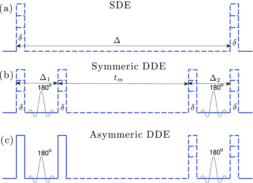
The dMRI signal in Eq. (4) can be obtained from the solution to Eq. (5). In the special case of SDE or DDE experiment with narrow pulse, q²(t) is either constant or piecewise constant, which leads to a closed-form solution to Eq. (5). Specifically, let $K≔\left[\begin{array}{cc}\hfill -k_{12}& k_{21}\hfill \\ \hfill k_{12}& -k_{21}\hfill \end{array}\right]$, and M(q) ≔ K − Dq² with $D=\left[\begin{array}{cc}\hfill D_1\hfill & \hfill 0\hfill \\ \hfill 0\hfill & \hfill D_2\hfill \end{array}\right]$. Then the dMRI signal obtained using a SDE sequence with narrow pulse, as shown in Fig. 1(a), is given by

$$S_{\text{SDE}}(q,T)={\mathbf{1}}^{\prime }\exp \left(M(q)T\right){\mathit{p}}^{\infty },$$ (6)

which is also the solution by Kärger,⁵ where q denotes the constant q-value, $\exp \left(A\right)$ denotes the matrix exponential function of a matrix A, 1 denotes a vector whose entries are all equal to one. For a DDE sequence with narrow pulse, as shown in Fig. 1(b), we denote the q-value between the first and second pair of pulses as q₁ and q₂, respectively, i.e., q(t) = q₁ for t ∈ [0, Δ₁] and q(t) = q₂ for t ∈ [T − T₂, T], where T = Δ₁ + Δ₂ + t_m, with t_m being the mixing time between the two pairs of pulses. Then the dMRI signal obtained for a DDE sequence is given by

$$\begin{array}{ccc}\hfill S_{\text{DDE}}(q_1,q_2,{\mathrm{\Delta }}_1,{\mathrm{\Delta }}_2,t_m)& =\hfill & {\mathbf{1}}^{\prime }\exp \left(M(q_2){\mathrm{\Delta }}_2\right)\exp \left(K{t}_m\right)\hfill \\ \hfill & \hfill & \times \exp \left(M(q_1){\mathrm{\Delta }}_1\right){\mathit{p}}^{\infty }.\hfill \end{array}$$ (7)

For completeness, we provide the closed-form expression for the matrix exponential exp(M(q)T) in Appendix B. In the more general case when q(t) is a continuous function of t, there is in general no closed-form solution for Eq. (5).

FIG. 1.

An illustration of three types of gradient sequences: (a) A standard SDE sequence with variable diffusion time and magnitude; (b) a symmetric DDE sequence with two symmetric pairs of pulses, where the diffusion time Δ₁, Δ₂ and the magnitude of the two pairs of pulses are identical, i.e., Δ₁ = Δ₂, q₁ = q₂, and the mixing time t_m and q_a are variable parameters; (c) an asymmetric DDE sequence, similar to the FEXI sequence in Ref. 12, where the magnitude for the first pair of pulses is fixed (indicated by solid lines), the diffusion time Δ₁ = Δ₂, and the mixing time and the magnitude of the second pair of pulses are variable.

C. On the cumulant expansion with water exchange

Although the expressions in Eqs. (6) and (7) can be directly used to model SDE and DDE signals with given experimental parameters, the complex expression of matrix exponentials is a major limitation to gain insights about choosing the optimal experimental parameters, especially for DDE sequences, which are characterized by multiple parameters such as diffusion time, mixing time, and gradient strength. A common approach to simplify the dMRI signal model and to gain insights about the role of experimental parameters is to use the cumulant expansion²⁷ expressed as follows:

$$\begin{array}{ccc}\hfill \ln S(q,T)& =\hfill & \mathrm{i}{⟨\varphi (T)⟩}_c-\frac{1}{2}{⟨\varphi {(T)}^2⟩}_c-\frac{\mathrm{i}}{6}{⟨\varphi {(T)}^3⟩}_c\hfill \\ \hfill & \hfill & +\frac{1}{24}{⟨\varphi {(T)}^4⟩}_c+\cdots ,\hfill \end{array}$$

where the cumulant moments ${⟨\varphi {(T)}^n⟩}_c$ can be expressed in terms of ordinary moments $\mathcal{E}(\varphi {(T)}^n)$. Typically, the probability distribution function of ϕ(T) is assumed to be symmetric. As a result, all the odd order moments $\mathcal{E}(\varphi {(T)}^{2n-1})$ are equal to zero. The second and fourth order cumulant moments are given by

$${⟨\varphi {(T)}^2⟩}_c=\mathcal{E}(\varphi {(T)}^2),$$ (8)

$${⟨\varphi {(T)}^4⟩}_c=\mathcal{E}(\varphi {(T)}^4)-3\mathcal{E}{(\varphi {(T)}^2)}^2,$$ (9)

respectively. Since the expression for the dMRI signal in SDE and DDE experiments is known, a general approach for computing the cumulant moments is to compute the Taylor-series expansion of S or ln S. But the complex expression for the dMRI signal, especially for DDE experiments, makes the derivation of the cumulant expansion extremely tedious. Consequently, we propose a different approach to derive the cumulant expansion by taking advantage of the proposed stochastic diffusion-and-exchange model in Eqs. (1) and (2).

1. On the second-order moment

From Eq. (3), the second order cumulant moment of ϕ(T) is given by

$$\begin{array}{ccc}\hfill \mathcal{E}({\varphi }^2(T))& =\hfill & {\int }_0^T{\int }_0^{T}q(t_1)q(t_2)\mathcal{E}\left(\sigma ({\mathit{x}}_{t_1})\sigma ({\mathit{x}}_{t_2})d{w}_{t_1}d{w}_{t_2}\right)\hfill \\ \hfill & =\hfill & {\int }_0^T{\int }_0^{T}q{(t)}^2\mathcal{E}\left(\sigma {({\mathit{x}}_t)}^2\right)dt.\hfill \end{array}$$ (10)

We note that

$$\begin{array}{ccc}\hfill \mathcal{E}(\sigma {({\mathit{x}}_t)}^2)& =\hfill & 2\sum _{i=1}^2\text{Prob}(s(t)=i)D_i\hfill \\ \hfill & =\hfill & 2(p_1{D}_1+p_2{D}_2)=:2\overline{D}.\hfill \end{array}$$

Thus, Eq. (10) is equal to

$$\mathcal{E}({\varphi }^2(T))=2\overline{D}{\int }_0^{T}q{(t)}^{2}dt=2\overline{D}b,$$ (11)

where the b-value $b≔{\int }_0^{T}q{(t)}^{2}dt$, which is equal to q²T in SDE experiments and $q_1^2{\mathrm{\Delta }}_1+q_2^2{\mathrm{\Delta }}_2$ in DDE experiments (under narrow pulse assumption). We remark that Eq. (11) implies that the second order moment does not contain information about the water exchange rate. Moreover, Eq. (11) also implies that the apparent diffusion coefficient (ADC) is given by

$$\text{ADC}≔\frac{\partial \mathcal{E}({\varphi }^2(T))}{2\partial b}{\mid }_{b=0}=\overline{D},$$ (12)

which is independent of the type of gradient waveform used. Similarly, one can show that Eq. (12) holds even if there are more than two components in the diffusion-exchange model, as long as the diffusion-exchange processes can be modeled by Eq. (1).

2. On the fourth-order moment

Due to the independence between $d{w}_{t_1}$ and $d{w}_{t_2}$ for t₁ ≠ t₂, the fourth-order moment $\mathcal{E}(d{w}_{t_1}d{w}_{t_2}d{w}_{t_3}d{w}_{t_4})$ is nonzero only if the set of indices {t₁, t₂, t₃, t₄} consists of two pairs of equal values, e.g., t₁ = t₂ and t₃ = t₄. Thus, we obtain

$$\mathcal{E}({\varphi }^4(T))=3{\int }_0^T{\int }_0^{T}q{(t_1)}^{2}q{(t_2)}^2\mathcal{E}(\sigma {({\mathit{x}}_{t_1})}^2\sigma {({\mathit{x}}_{t_2})}^2)d{t}_{1}d{t}_2.$$ (13)

To compute the correlation $\mathcal{E}(\sigma {({\mathit{x}}_{t_1})}^2\sigma {({\mathit{x}}_{t_2})}^2)$, we assume that t₁ ≤ t₂. Then,

$$\begin{array}{ll}\hfill & \mathcal{E}(\sigma {({\mathit{x}}_{t_1})}^2\sigma {({\mathit{x}}_{t_2})}^2)\hfill \\ \hfill & =p_1^{\infty }\left(\right.p_{11}(t_1)p_{11}(t_2-t_1)4D_1^2+p_{11}(t_1)p_{12}(t_2-t_1)4D_1{D}_2\hfill \\ \hfill & +p_{12}(t_1)p_{21}(t_2-t_1)4D_1{D}_2+p_{12}(t_1)p_{22}(t_2-t_1)4D_2^2\left)\right.\hfill \\ \hfill & +p_2^{\infty }\left(\right.p_{21}(t_1)p_{11}(t_2-t_1)4D_1^2+p_{21}(t_1)p_{12}(t_2-t_1)4D_1{D}_2\hfill \\ \hfill & +p_{22}(t_1)p_{21}(t_2-t_1)4D_1{D}_2+p_{22}(t_1)p_{22}(t_2-t_1)4D_2^2\left)\right.\hfill \\ \hfill & =4{(p_1^{\infty }{D}_1+p_2^{\infty }{D}_2)}^2+4p_1^{\infty }{p}_2^{\infty }{(D_1-D_2)}^2{e}^{-k(t_2-t_1)}.\hfill \end{array}$$ (14)

To further simplify Eq. (13), we define $\text{Var}(D)≔p_1^{\infty }{p}_2^{\infty }{(D_1-D_2)}^2$, which is equal to the variance of the diffusivities. Then, we introduce the following function:

$$c(t)≔{\overline{D}}^2+\text{Var}(D)e^{-kt}$$ (15)

for t ∈ [−T, T], which is the autocorrelation function for $\sigma {({\mathit{x}}_t)}^2$ in Eq. (14) scaled by $\frac{1}{4}$. Thus, Eq. (13) can be written as

$$\mathcal{E}({\varphi }^4(T))=12{\int }_0^T{\int }_0^{T}q{(t_1)}^{2}q{(t_2)}^{2}c(|t_1-t_2|)d{t}_{1}d{t}_2.$$ (16)

Using a similar methodology as in our earlier work,^22,28 we can further simplify the above equation to

$$\mathcal{E}({\varphi }^4(T))=24{\int }_0^{T}c(t)q_4(t)dt,$$ (17)

where q₄(t) is defined as

$$q_4(t):={\int }_0^T{q}^2(t_1)q^2(t_1+t)d{t}_1,$$

where we assume q(t) = 0 for t ≥ T. We note that the fourth-order moment is a function of the exchange rate and the fourth-order autocorrelation function of q(t). For completeness, we provide a general expression for other higher order moments in Appendix C. By applying Eqs. (17) and (11) to Eq. (9), we obtain

$${⟨\varphi {(T)}^4⟩}_{\mathrm{c}}=24\text{Var}(D){\int }_0^T{e}^{-kt}{q}_4(t)dt,$$ (18)

which shows the dependence of the fourth-order cumulant on the exchange rate and the gradient sequence.

D. General signal expression

At this point, we can define a signal expression that generalizes across all gradient waveforms

$$\ln S=-\overline{D}b+\frac{1}{2}\text{Var}(D)h(\cdot )b^2+O(b^3),$$ (19)

where h(⋅) denotes an exchange-sensitivity function of the gradient sequence which is defined by

$$h(\cdot )=2{\int }_0^T{e}^{-kt}{\tilde{q}}_4(t)dt$$ (20)

and

$${\tilde{q}}_4(t)=\frac{q_4(t)}{b^2}.$$ (21)

The expansion in Eq. (19) is based on the assumption of low b-values so that the third or higher order terms of b are negligible compared to b². The term ${\tilde{q}}_4(t)$ contains the timing information of the gradient waveform. Note that the ability to observe exchange relies on the presence of intra-voxel variance in diffusivity, i.e., Var(D) > 0. Finally, in the absence of exchange, or for very slow exchange where kT ≪ 1, we get e^−kt ≈ 1 for 0 ≤ t ≤ T and thus h(⋅) = 1. In the presence of exchange, h(⋅) < 1, and in the case of exchange much faster than the gradient waveform, we get h(⋅) → 0 meaning that the system will appear as a single system without any observable diffusional variance.

Note the similarity of Eq. (19) to the diffusional kurtosis model²⁹

$$\ln S\approx -D_{\text{app}}b+\frac{1}{6}{D}_{\text{app}}^2{K}_{\text{app}}{b}^2,$$ (22)

where $D_{\text{app}}=\overline{D}$ in our notation and $K_{\text{app}}=6\text{Var}(D)/{\overline{D}}^2$ in the absence of exchange. However, the presence of exchange reduces the apparent kurtosis according to

$$K_{\text{app}}(\cdot )=3\frac{\text{Var}(D)}{{\overline{D}}^2}h(\cdot ),$$ (23)

which depends on the gradient sequences and diffusion time.

1. Defining a generalized exchange weighting time

To further analyze the effect of water-exchange in dMRI signals, we consider the situation when e^−kt ≈ 1 − kt for t ∈ [0, T]. Then we get

$$\begin{array}{ccc}\hfill h(\cdot )& \approx \hfill & 2{\int }_0^T(1-kt){\tilde{q}}_4(t)dt,\hfill \\ \hfill & =\hfill & 1-k\mathrm{\Gamma },\hfill \end{array}$$ (24)

where we define the exchange weighting time Γ as

$$\mathrm{\Gamma }≔2{\int }_0^{T}t{\tilde{q}}_4(t)dt.$$ (25)

Accordingly, we have an approximation of Eq. (19) as

$$\ln S\approx -\overline{D}b+\frac{1}{2}\text{Var}(D)(1-k\mathrm{\Gamma })b^2.$$ (26)

In the following, we will compute the function h(⋅) and the signal model in Eq. (26) for three types of sequences shown in Fig. 1, which includes a standard SDE sequence in Fig. 1(a), a DDE sequence with two identical pairs of pulses in Fig. 1(b) where Δ₁ = Δ₂, and a FEXI type of DDE sequence in Fig. 1(c) where the magnitude of the first pair of pulses is fixed (indicated by solid lines). Although the signal model for SDE experiments has been well studied in Refs. ¹ and ³⁰, comparing the different Γ’s will highlight the sensitivity of dMRI signal to water exchange rate for these gradient waveforms.

2. Signal expression for SDE sequences

For the SDE sequence shown in Fig. 1(a), if the pulse width δ is negligibly small, then h(⋅) is given by

$$h_{\text{SDE}}(\tau )=\frac{2}{\tau }-\frac{2}{{\tau }^2}+\frac{2}{{\tau }^2}{e}^{-\tau },$$ (27)

where τ ≔ kΔ. The corresponding exchange-weighted time is equal to

$${\mathrm{\Gamma }}_{\text{SDE}}=\frac{1}{3}\mathrm{\Delta }.$$ (28)

In the case of finite pulse width, the exchange-weighted time is equal to

$${\mathrm{\Gamma }}_{\text{SDE}}=\frac{1}{3}f(\delta ,\mathrm{\Delta }),$$ (29)

where

$$f(\delta ,\mathrm{\Delta })={(\mathrm{\Delta }-\frac{1}{3}\delta )}^{-2}({\mathrm{\Delta }}^3-{\mathrm{\Delta }}^2\delta +\frac{2}{3}{\delta }^2\mathrm{\Delta }-\frac{4}{21}{\delta }^3).$$

If Δ ≫ δ, $f(\delta ,\mathrm{\Delta })\approx (\mathrm{\Delta }-\frac{1}{3}\delta )$ which is equal to the equivalent diffusion time.

3. Signal expression for DDE sequences

First, we consider the narrow-pulse situation when the diffusion time Δ₁ = Δ₂ = Δ, T = 2Δ + t_m, and the b-values corresponding to the two pairs of pulses are given by b₁ and b₂, respectively. Following Eq. (18), we obtain

$$h_{{\text{DDE}}_{\mathrm{A}}}(\cdot )=\frac{b_1^2+b_2^2}{b^2}{h}_{\text{SDE}}({\tau }_1)+\frac{2b_1{b}_2}{b^2}{h}_{\text{DDE}}({\tau }_1,\tau ),$$ (30)

where we define

$$h_{\text{DDE}}({\tau }_1,\tau )≔\frac{1}{{\tau }_1^2}(e^{-\tau +2{\tau }_1}+e^{-\tau }-2e^{-\tau +{\tau }_1}),$$

τ₁ = kΔ₁, τ = kT, b = b₁ + b₂, and the subindex DDE_A denotes the asymmetric DDE sequence. The corresponding exchange-weighted time is equal to

$${\mathrm{\Gamma }}_{{\text{DDE}}_{\mathrm{A}}}=\frac{b_1^2+b_2^2}{3b^2}{\mathrm{\Delta }}_1+\frac{2b_1{b}_2}{b^2}({\mathrm{\Delta }}_1+t_m).$$

In the special case when b₁ = b₂, the corresponding exchange weighting time is

$${\mathrm{\Gamma }}_{{\text{DDE}}_{\mathrm{S}}}=\frac{2}{3}{\mathrm{\Delta }}_1+\frac{1}{2}{t}_m.$$

The exchange weighting time can be generalized to the situation when the pulse width is finite as follows:

$$\begin{array}{ccc}\hfill {\mathrm{\Gamma }}_{{\text{DDE}}_{\mathrm{A}}}& =\hfill & \frac{b_1^2+b_2^2}{b^2}f(\delta ,{\mathrm{\Delta }}_1)+\frac{2b_1{b}_2}{b^2}({\mathrm{\Delta }}_1+t_m)\hfill \\ \hfill & \approx \hfill & \frac{b_1^2+b_2^2+6b_1{b}_2}{3b^2}{\mathrm{\Delta }}_1+\frac{2b_1{b}_2}{b^2}{t}_m-\frac{b_1^2+b_2^2}{9b^2}\delta ,\hfill \end{array}$$

when Δ ≫ δ. For symmetric DDE sequences, i.e., when b₁ = b₂, the corresponding exchange-weighted time is

$${\mathrm{\Gamma }}_{{\text{DDE}}_{\mathrm{S}}}=\frac{2}{3}{\mathrm{\Delta }}_1+\frac{1}{2}{t}_m-\frac{1}{18}\delta .$$

4. On the relation with FEXI-signal model

If the first pair of pulses of the asymmetric DDE sequence is fixed, then the dMRI signal can be normalized with respect to signal from the first SDE sequence as

$$\begin{array}{ccc}\hfill & \hfill & \ln S_{{\text{DDE}}_{\mathrm{A}}}(\cdot )-\ln S_{\text{SDE}}(b_1,k{\mathrm{\Delta }}_1)\hfill \\ \hfill & \approx \hfill & (-\overline{D}+2\text{Var}(D)h_{\text{DDE}}(k{\mathrm{\Delta }}_1,kT)b_1)b_2\hfill \\ \hfill & \approx \hfill & (-\overline{D}+2\text{Var}(D)(1-k({\mathrm{\Delta }}_1+t_m))b_1)b_2,\hfill \end{array}$$ (31)

where the last equation is obtained by using h_DDE(kΔ₁, kT) ≈ 1 − k(Δ₁ + t_m).

A similar model was proposed in Ref. 12, which is given by

$$\begin{array}{ccc}\hfill & \hfill & \ln S_{\text{FEXI}}(\cdot )-\ln S_{\text{SDE}}(b_1,k{\mathrm{\Delta }}_1)\hfill \\ \hfill & \approx \hfill & -\overline{D}(1-{\sigma }_f\exp (-\text{AXR}\times t_m))b_2\hfill \\ \hfill & \approx \hfill & (-\overline{D}+\overline{D}{\sigma }_f-\overline{D}{\sigma }_f{t}_m\text{AXR})b_2.\hfill \end{array}$$ (32)

Since Δ₁ is fixed and t_m is changing in the experiment, the coefficients of t_m in Eqs. (31) and (32) should match with each other. Consequently we obtain

$$\begin{array}{ccc}\hfill \overline{D}{\sigma }_f& =\hfill & 2\text{Var}(D)(1-k{\mathrm{\Delta }}_1)b_1,\hfill \\ \hfill \overline{D}{\sigma }_f\text{AXR}& =\hfill & 2\text{Var}(D)k{b}_1.\hfill \end{array}$$

Thus, the following holds

$$\text{AXR}=\frac{k}{1-k{\mathrm{\Delta }}_1},$$ (33)

which is approximately equal to k if kΔ₁ ≪ 1. In the more general case, Eq. (33) can be applied to compute k using the estimated AXR and Δ₁.

E. Optimal sequence parameters

For the three sequences above, we will design the optimal acquisition parameters to maximize the sensitivity to water exchange. This will also allow for comparison of these sequences for practical applications. Optimality in this case is defined as the set of parameters that provide maximal signal decay due to water exchange. To obtain a fair comparison, we impose the following constraints on all the sequences: first, the diffusion time T is only allowed to change in the interval [T_min, T_max]; second, the maximal b-value has an upper bound b_max. Thus, a natural constraint on Δ₁ in DDE experiments is ${\mathrm{\Delta }}_1\le \frac{1}{2}{T}_{min}$. We assume T_min is small so that the exchange sensitivity function $h_{\text{SDE}}(k{T}_{min})\approx 1-\frac{1}{3}k{T}_{min}$. The attenuation due to exchange will be the objective function by which these sequences will be compared.

1. SDE sequences

From Eqs. (19) and (27), the dMRI signal for a SDE sequence is given by

$$\ln S_{\text{SDE}}(b,kT)\approx -\overline{D}b+\frac{1}{2}\text{Var}(D)h_{\text{SDE}}(kT)b^2.$$ (34)

Thus, the maximal signal difference under the given constraints is approximately given by

$$e_{\text{SDE}}=\frac{1}{2}\text{Var}(D)(h_{\text{SDE}}(k{T}_{min})-h_{\text{SDE}}(k{T}_{max}))b_{max}^2.$$ (35)

If kT_max ≫ 1, i.e., if the exchange-sensitivity function h_SDE(kT_max) ≈ 0, then

$$\begin{array}{ccc}\hfill e_{\text{SDE}}& \approx \hfill & \frac{1}{2}\text{Var}(D)h_{\text{SDE}}(k{T}_{min})b_{max}^2\hfill \\ \hfill & \approx \hfill & \frac{1}{2}\text{Var}(D)(1-\frac{1}{3}k{T}_{min})b_{max}^2.\hfill \end{array}$$ (36)

On the other hand, if kT_max ≪ 1, i.e., if the exchange-sensitivity function $h_{\text{SDE}}(k{T}_{max})\approx 1-\frac{1}{2}k{T}_{max}$, then

$$e_{\text{SDE}}\approx \frac{1}{6}\text{Var}(D)k(T_{max}-T_{min})b_{max}^2.$$ (37)

2. DDE sequences

From Eqs. (19) and (30), the dMRI signal for asymmetric DDE sequence is given by

$$\begin{array}{ccc}\hfill \ln S_{{\text{DDE}}_{\mathrm{A}}}& \approx \hfill & -\overline{D}b+\frac{1}{2}\text{Var}(D)\left(\right.h_{\text{SDE}}(k{\mathrm{\Delta }}_1)(b_1^2+b_2^2)\hfill \\ \hfill & \hfill & +2b_1{b}_2{h}_{\text{DDE}}(k{\mathrm{\Delta }}_1,kT)\left)\right..\hfill \end{array}$$

Thus, the signal difference for asymmetric DDE sequences is given by

$$e_{{\text{DDE}}_{\mathrm{A}}}\approx \text{Var}(D)(h_{\text{DDE}}(k{\mathrm{\Delta }}_1,k{T}_{min})-h_{\text{DDE}}(k{\mathrm{\Delta }}_1,k{T}_{max}))b_1{b}_2.$$

Moreover, the maximum value of the product b₁b₂ is equal to $\frac{1}{4}{b}_{max}^2$, when $b_1=b_2=\frac{1}{2}{b}_{max}$. In this case, the signal difference $e_{{\text{DDE}}_{\mathrm{A}}}$ is equal to the corresponding result with symmetric DDE sequences. Thus, we denote the signal difference for both types of DDE sequences as

$$e_{\text{DDE}}=\frac{1}{4}\text{Var}(D)(h_{\text{DDE}}(k{\mathrm{\Delta }}_1,k{T}_{min})-h_{\text{DDE}}(k{\mathrm{\Delta }}_1,k{T}_{max}))b_{max}^2.$$ (38)

If kT_max ≫ 1, i.e., h_DDE(kΔ₁, kT_max) ≈ 0, then

$$\begin{array}{ccc}\hfill e_{\text{DDE}}& \hfill & \approx \frac{1}{4}\text{Var}(D)h_{\text{DDE}}(k{\mathrm{\Delta }}_1,k{T}_{min})b_{max}^2\hfill \\ \hfill & \hfill & \approx \frac{1}{4}\text{Var}(D)(1-k(T_{min}-{\mathrm{\Delta }}_1))b_{max}^2.\hfill \end{array}$$

Thus, the optimal value of Δ₁ that maximizes e_DDE is obtained when ${\mathrm{\Delta }}_1=\frac{1}{2}{T}_{min}$. In this case,

$$e_{\text{DDE}}\approx \frac{1}{4}\text{Var}(D)(1-\frac{1}{2}k{T}_{min})b_{max}^2.$$ (39)

On the other hand, if kT_max ≪ 1, then

$$e_{\text{DDE}}(\cdot )\approx \frac{1}{4}\text{Var}(D)k(T_{max}-T_{min})b_{max}^2.$$ (40)

3. Comparing SDE and DDE sequences

If kT_max ≫ 1, then the maximum attenuation for SDE and DDE sequence is given by Eqs. (36) and (39), respectively. In this case,

$$e_{\text{SDE}}>e_{\text{DDE}}.$$

If kT_max ≪ 1, by comparing Eqs. (37) and (40), we obtain that

$$e_{\text{SDE}}<e_{\text{DDE}}.$$

Thus, e_SDE is less sensitive to k than e_DDE at short-time scale but has a stronger attenuation at long-time scale.

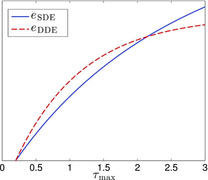
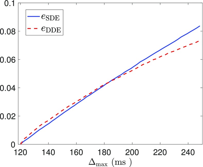
As an illustration of the above results, we plot e_SDE, e_DDE from Eqs. (35) and (38) for different values of τ_max in Fig. 2 with a fixed value for τ_min at τ_min = 0.2. The result shows that the DDE sequence has higher sensitivity than SDE sequence at short-time scales but has lower sensitivity at long-time scale.

FIG. 2.

A comparison of e_SDE and e_DDE from Eqs. (35) and (38), respectively, with τ_min = 0.2 and arbitrary values for Var(D) and b_max. The plots show that e_DDE > e_SDE for small τ_max, and e_DDE < e_SDE for large τ_max.

III. EXPERIMENTS

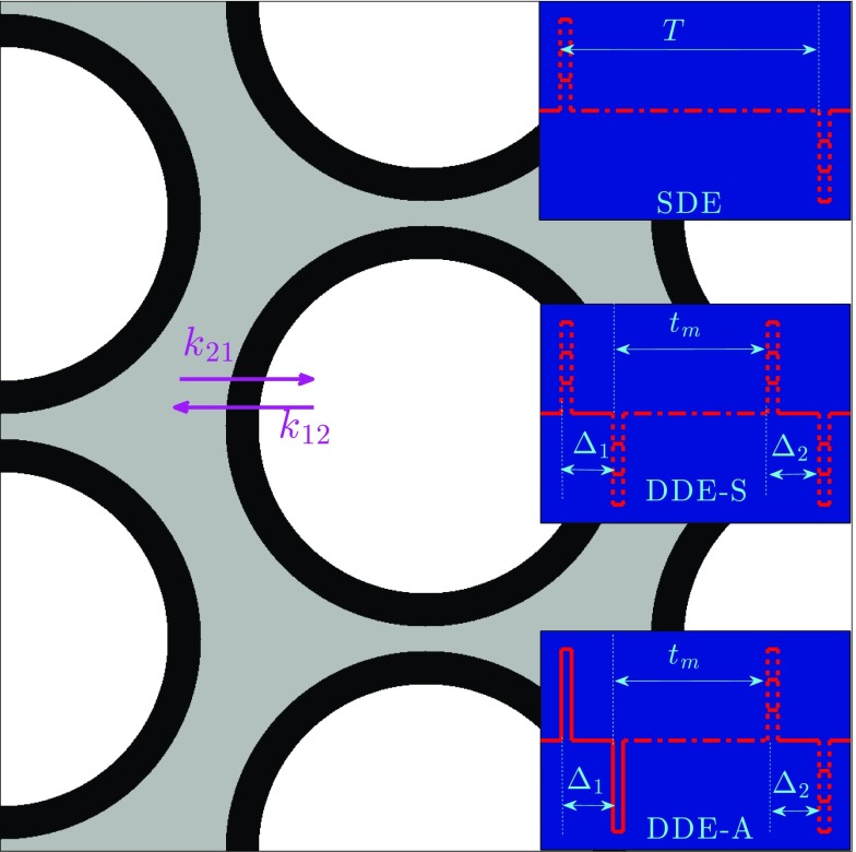
We validated the proposed results using Monte Carlo simulations performed on a synthetic structure using a method similar to the approach described in Ref. 8. Figure 3 shows a partial field of view of the synthetic axonal packing structure used in our simulation, inset with illustration of the pulse sequences for simulating the dMRI signal. The axon diameter was fixed to 2.5 μm, and the intra- and extra-axonal volume fractions were 0.7 and 0.3, respectively. The membrane permeability was chosen such that the effective intra-to-extra and extra-to-intra cellular exchange time was $t_{12}=\frac{1}{k_{12}}=322\text{\hspace{0.17em}ms}$ (i.e., k₁₂ = 0.0031 ms⁻¹) and $t_{21}=\frac{1}{k_{21}}=139\text{\hspace{0.17em}ms}$ (i.e., k₂₁ = 0.0072 ms⁻¹), respectively. These values fit in the range of exchange rates estimated from biological tissue.^31–33 The diffusivity of the spins was set to 3 μm²/ms. Both SDE and DDE modulated signals were computed using the simulated diffusion trajectories. The pulse width for both sequences was fixed to 0.45 ms, and the diffusion or mixing time was changed for measuring the exchange rate. In the SDE experiments, the diffusion time was chosen in the interval T ∈ [120, 240] ms, i.e., T_min = 120 ms and T_max = 240 ms, and b_max = 10 ms/μm².

FIG. 3.

Illustration of the synthetic tissue structure with permeable boundaries along with schematic for the SDE, DDE_S, and DDE_S gradient sequences used for encoding the dMRI signals.

We also examined the signal due to symmetric and asymmetric DDE sequences, as shown in Fig. 3. For the symmetric DDE sequence, we applied the proposed result to set ${\mathrm{\Delta }}_1=\frac{T_{min}}{2}=60\text{\hspace{0.17em}ms}$. For comparison, we also applied a non-optimal value for Δ₁ with Δ₁ = 30 ms. For the asymmetric SDE sequence, we used the following optimal parameters: Δ₁ = 60 ms and b₁ = 5 ms/μm². For comparison, we also used a non-optimal sequence with b₁ = 2.5 ms/μm².

The purpose of this experiment is (1) to examine the performance of the models in Eqs. (6) and (7) in fitting simulated signals and in estimating the water exchange rate, (2) to examine the cumulant expansion of SDE and DDE signals and compare them with the complete signal models, (3) to validate the optimality of the proposed experimental parameters, (4) to compare the signal differences, i.e., e_SDE and e_DDE, between SDE and DDE sequences under the same constraints.

IV. RESULTS

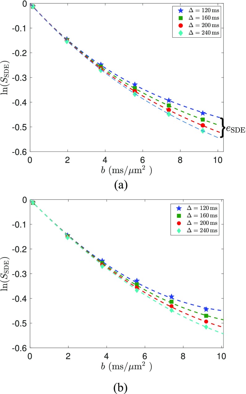
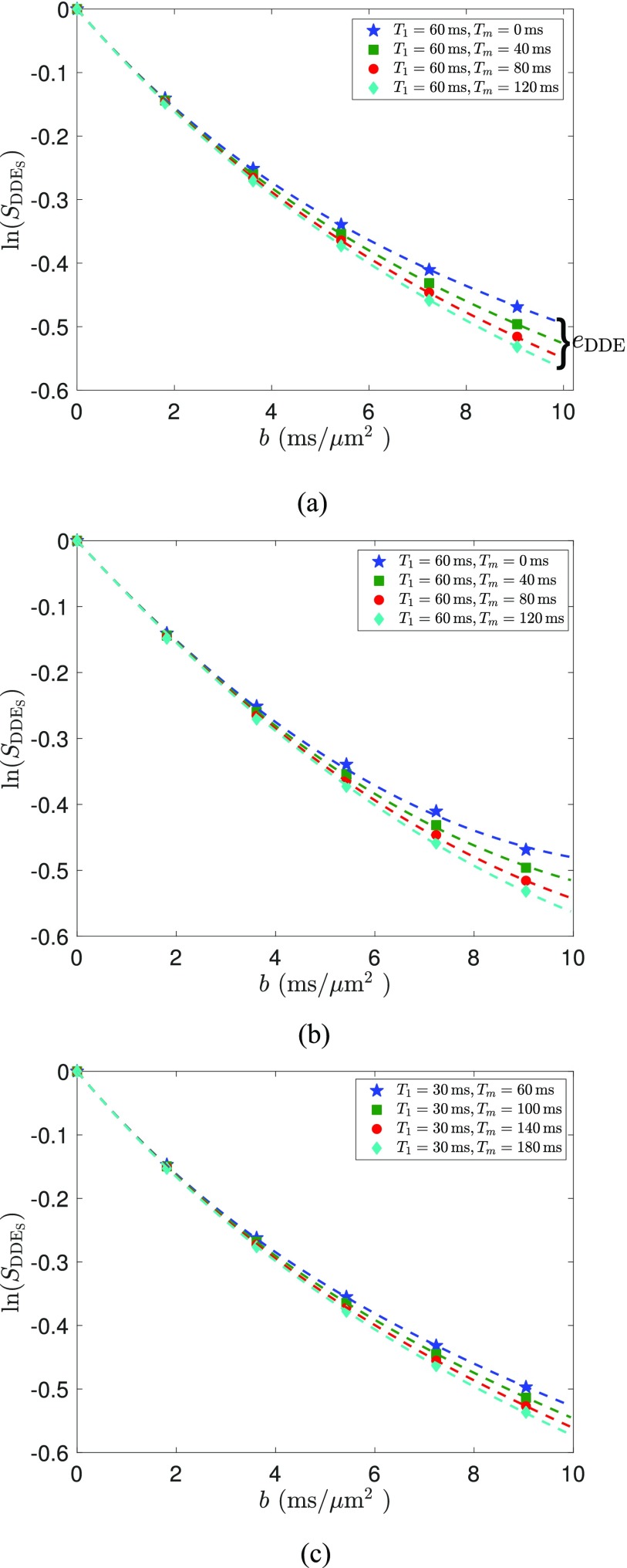
The dMRI signal for the SDE sequence is illustrated in Fig. 4, where the markers show the Monte Carlo simulated data, the dashed lines in Fig. 4(a) are the estimated signal using the complete signal model from (6), and Fig. 4(b) shows the signal using the cumulant expansion (19) with h_SDE given by (27). The closed-form expression for the matrix exponential exp(M(q)Δ) in (6) is provided in Appendix A. The model parameters were estimated using the lsqnonlin algorithm implemented in MATLAB®. We note that the estimated signal in Fig. 4(a) fits nicely to the simulated data. The cumulant expansion in Fig. 4(b) has a slight fitting error at high b-values due to the truncation of higher order terms. The estimated model parameters in Fig. 4(a) were D₁ = 0 μm²/ms, D₂ = 0.2819 μm²/ms, k₁₂ = 0.0034 ms⁻¹, and k₂₁ = 0.0080 ms⁻¹. The estimated parameters for the cumulant expansion were D₁ = 0.001 μm²/ms, D₂ = 0.2067 μm²/ms, k₁₂ = 0.0040 ms⁻¹, and k₂₁ = 0.0064 ms⁻¹. Both are close to the true exchange rates. The estimated apparent diffusivity is much lower than the set value of intrinsic diffusivity, due to restrictions and hindrances from the tissue boundaries. We remark that these signals all have similar slopes near b = 0, which indicates that the apparent diffusivity is nearly constant at this time scale as shown in (12). Therefore, the assumption of constant diffusivity is valid in this experiment.

FIG. 4.

The markers show the simulated SDE signal. The dashed lines in (a) show the estimated signals (S_SDE) using the complete signal model (6). (b) shows the estimated signals (S_SDE) using the cumulant expansion (19) with h_SDE given by (27).

Figures 5(a) and 5(b) illustrate the simulated signal for symmetric DDE sequences with Δ₁ = 60 ms using the complete signal model (7) and the cumulant expansion (19), respectively. We note that the cumulant expansion has slightly higher fitting error at high b-values. The estimated model parameters corresponding to Fig. 5(a) are D₁ = 0.0130 μm²/ms, D₂ = 0.3149 μm²/ms, k₁₂ = 0.0022 ms⁻¹, and k₂₁ = 0.0064 ms⁻¹. The estimated parameters for Fig. 5(a) are D₁ = 0.0037 μm²/ms, D₂ = 0.1955 μm²/ms, k₁₂ = 0.0028 ms⁻¹, and k₂₁ = 0.0040 ms⁻¹. The estimated exchange rates are slightly lower than the underlying true values.

FIG. 5.

The markers in (a) and (b) show the simulated signals using symmetric DDE sequences with the theoretically optimal Δ₁ = 60 ms and the markers in (c) are the simulated signal with Δ₁ = 30 ms. The dashed lines in (a) and (c) illustrate the estimated signals using the complete signal model (7). The dashed lines in (b) are estimated signals using the cumulant expansion (19) with h(⋅) given by (30).

Figure 5(c) illustrates the simulated and estimated signal using (7) with Δ₁ = 30 ms, which is suboptimal according to the theoretical analysis in Sec. II E 2. The estimated model parameters were D₁ = 0.0220 μm²/ms, D₂ = 0.3369 μm²/ms, k₁₂ = 0.0012 ms⁻¹, and k₂₁ = 0.0040 ms⁻¹. We note that the signal variance is much smaller in Fig. 5(c) for the suboptimal condition compared to the optimal parameters in Fig. 5(a). This demonstrates the advantage of using optimized parameters for more sensitivity to exchange.

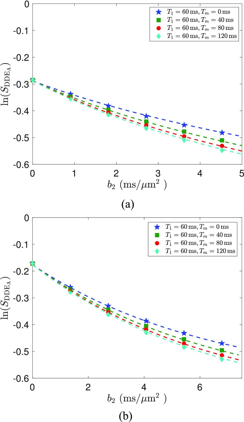
Figures 6(a) and 6(b) illustrate the simulated signal for asymmetric DDE sequences versus b₂ with b₁ fixed at b₁ = 5, and 2.5 ms/μm², respectively. The maximal b-value in both cases is equal to 10 ms/μm². Similar to the case of symmetric DDE sequences, the dashed lines are the estimated results from Eq. (7), which all fit nicely with the simulated data shown by the markers. The estimated model parameters corresponding to Fig. 6(a) are D₁ = 0.0158 μm²/ms, D₂ = 0.3675 μm²/ms, k₁₂ = 0.0028 ms⁻¹, and k₂₁ = 0.0115 ms⁻¹. The estimated model parameters for Fig. 6(b) are equal to D₁ = 0 μm²/ms, D₂ = 0.2494 μm²/ms, k₁₂ = 0.0043 ms⁻¹, and k₂₁ = 0.0085 ms⁻¹.

FIG. 6.

The dashed lines in (a) show the estimated signal using symmetric DDE sequences with the theoretically optimal b₁ = 10 ms/μm², which fit nicely to the signal from simulated data shown by the markers. Similarly, (b) shows the signals with a non-optimal value b₁ = 5 ms/μm², which leads to a slightly weaker signal difference, i.e., e_DDE, compared to (a).

We note that the difference between signals, i.e., e_DDE, with t_m = 120 ms and t_m = 0 ms at b₂ = 5 ms/μm² in Fig. 6(a) is equal to 0.0417, whereas the corresponding value from Fig. 6(b) at b₂ = 7.5 ms/μm² has a smaller value at 0.0373, which supports the optimality of b₁ = 5 ms/μm² in maximizing signal difference.

Figure 7 illustrates the comparison between e_SDE and e_DDE with the optimal parameters and the maximal diffusion time chosen in the interval T_max ∈ [120, 240] ms. It shows a very similar feature as in Fig. 2, though the theoretical analysis in Fig. 2 did not consider the third or higher order terms. More specifically, Fig. 7 shows that the signal change in a DDE sequence is more sensitive to water exchange than a SDE sequence when Δ_max is small. But the SDE sequence provides larger signal changes at long time scale.

FIG. 7.

A comparison of the signal differences e_SDE and e_DDE with T_min = 120 ms, b_max = 20 ms/μm², and T_max ∈ [120, 240] ms. This provides an experimental validation of the results from Fig. 2.

V. DISCUSSION AND CONCLUSIONS

In this paper, we investigated a model for the diffusion-and-exchange stochastic processes of water molecules. We derived a generalized expression of Kärger’s model for the temporal evolution of the dMRI signal using any type of gradient sequence. We also derived analytical solutions for special case of SDE and DDE sequences. Moreover, we also proposed a novel solution for computing the cumulant expansion of dMRI signal using the stochastic evolution process without taking Taylor’s series expansion from the complex signal models. Based on this general solution, we derived the cumulant expansion for the dMRI signal for SDE as well as symmetric and asymmetric DDE sequences. The cumulant expansions show that the water exchange rate is related to the linear coefficient of the b-value for asymmetric DDE sequences, whereas it involves the quadratic terms for SDE and symmetric DDE sequences. Moreover, the cumulant expansions also provide the exact relation between the AXR from the FEXI approach and the true water exchange rate.

From the cumulant expansions, we also computed the optimal parameters for the DDE sequences under realistic constraints on the b-values and diffusion time, in order to provide maximal signal difference for increased sensitivity to water exchange. For the symmetric DDE sequence, we showed that the optimal diffusion time Δ₁ should be set to its upper bound at $\frac{1}{2}{T}_{min}$. For the asymmetric DDE sequences, the optimal value of b₁ is equal to $\frac{1}{2}{b}_{max}$. Moreover, we also showed that the signal from a DDE sequence with optimal parameters is more sensitive to water exchange than the signal from the SDE sequence.

Finally, we note that a limitation of the present work is the assumption of constant diffusion coefficients for each compartment in the diffusion-exchange model. An important future direction is to explore the application of more realistic models that take into account restrictions or hindrances in the diffusion processes in situations with fast exchange rate. Moreover, generalizations to multiple components, anisotropic diffusivities, and vector-valued gradient waveforms, which are important for estimation of microscopic anisotropy,^34,35 will also be explored in our future work.

APPENDIX A: PROOF OF THE GENERALIZED KÄRGER MODEL IN SEC. II B

Without loss of generality, we will only derive the derivative $\frac{\partial S_1(q,t)}{\partial t}$. By definition,

$$S_1(q,t+{\delta }_t)=\sum _{j=1}^2{p}_j^{\infty }{p}_{j1}(t+{\delta }_t)\mathcal{E}(e^{\mathrm{i}\varphi (t+{\delta }_t)}\mid s(t+{\delta }_t)=1,s(0)=j).$$

We denote $\varphi (t,t+{\delta }_t)≔{\int }_t^{t+{\delta }_t}q(\tau )\sigma (\mathit{x}(\tau ))\eta (\tau )d\tau$. Then, it holds that ϕ(t + δ_t) = ϕ(t) + ϕ(t, t + δ_t) and ϕ(t) is independent of ϕ(t, t + δ_t). Thus, it holds that

$$\begin{array}{ccc}\hfill & \hfill & S_1(q,t+{\delta }_t)\hfill \\ \hfill & \hfill & =\sum _{j=1}^2\sum _{k=1}^2{p}_j^{\infty }{p}_{jk}(t)p_{k1}({\delta }_t)\mathcal{E}(e^{\mathrm{i}\varphi (t)}\mid s(t)=k,s(t+{\delta }_t)=j)\hfill \\ \hfill & \hfill & \times \mathcal{E}(e^{\mathrm{i}\varphi (t,t+{\delta }_{\mathrm{t}})}\mid s(t+{\delta }_t)=1,s(t)=k)\hfill \\ \hfill & \hfill & =S_1(q,t)p_{11}({\delta }_t)\mathcal{E}(e^{\mathrm{i}\varphi (t,t+{\delta }_t)}\mid s(t+{\delta }_t)=1,s(t)=1)\hfill \\ \hfill & \hfill & +S_2(q,t)p_{21}({\delta }_t)\mathcal{E}(e^{\mathrm{i}\varphi (t,t+{\delta }_t)}\mid s(t+{\delta }_t)=1,s(t)=2).\hfill \\ \hfill & \hfill & \hfill \end{array}$$ (A1)

By discretizing Eq. (2), we obtain that

$$\begin{array}{ccc}\hfill p_{11}({\delta }_t)& =\hfill & p_{11}(0)(1-k_{12}{\delta }_t)+p_{12}(0)k_{21}{\delta }_t+o({\delta }_t)\hfill \\ \hfill & =\hfill & 1-k_{12}{\delta }_t+o({\delta }_t).\hfill \end{array}$$

To derive $\mathcal{E}(e^{\mathrm{i}\varphi (t,t+{\delta }_t)}\mid s(t+{\delta }_t)=1,s(0)=1)$, we define the event $\mathcal{A}(t,{\delta }_t)≔\left\{\exists t_1\in \left[t,t+{\delta }_t\right]\text{s.t.}s(t_1)\ne s(t)\right\}$, i.e., $\mathcal{A}(t,{\delta }_t)$ denotes the event that water exchange happens during the interval [t, t + δ_t] with given boundary conditions s(t) = 1, s(t + δ) = 1. Let ${\mathcal{A}}^c(t,{\delta }_t)$ denote the complementary event to $\mathcal{A}(t,{\delta }_t)$. Using Bayes’ rule, we obtain that

$$\begin{array}{ccc}\hfill & \hfill & \mathcal{E}(e^{\mathrm{i}\varphi (t,t+{\delta }_t)}\mid s(t+{\delta }_t)=1,s(t)=1)\hfill \\ \hfill & \hfill & =\text{Prob}(\mathcal{A}(t,{\delta }_t)\mid s(t)=1,s(t+{\delta }_t)=1)\mathcal{E}(e^{\mathrm{i}\varphi (t,t+{\delta }_t)}\mid s(t+{\delta }_t)=1,s(t)=1,\mathcal{A}(t,{\delta }_t))\hfill \\ \hfill & \hfill & +\text{\hspace{0.17em}Prob}({\mathcal{A}}^c(t,{\delta }_t)\mid s(t)=1,s(t+{\delta }_t)=1)\times \mathcal{E}(e^{\mathrm{i}\varphi (t,t+{\delta }_t)}\mid s(t+{\delta }_t)=1,s(t)=1,{\mathcal{A}}^c(t,{\delta }_t)).\hfill \end{array}$$

We note that, for short δ_t, the probability of exchange during the interval [t, t + δ_t] with the boundary condition that s(t + δ_t) = 1, s(t) = 1 is about zeros, i.e.,

$$\text{\hspace{0.17em}Prob}(\mathcal{A}(t,{\delta }_t)\mid s(t)=1,s(t+{\delta }_t)=1)=\frac{\text{\hspace{0.17em}Prob}(s(t+{\delta }_t)=1\mid s(t)=1)-\text{\hspace{0.17em}Prob}({\mathcal{A}}^c(t,{\delta }_t)\mid s(t)=1)}{\text{\hspace{0.17em}Prob}(s(t+{\delta }_t)=1\mid s(t)=1)}$$

is of order o(δ_t). Moreover,

$$\begin{array}{ccc}\hfill & \hfill & \mathcal{E}(e^{\mathrm{i}\varphi (t,t+{\delta }_t)}\mid s(t+{\delta }_t)=1,s(t)=1,{\mathcal{A}}^c(t,{\delta }_t))\hfill \\ \hfill & \hfill & =\exp (-{\int }_t^{t+{\delta }_t}q{(\tau )}^{2}ds{D}_1)=1-q{(t)}^2{D}_1{\delta }_t+o({\delta }_t).\hfill \end{array}$$

Thus,

$$\begin{array}{ccc}\hfill & \hfill & p_{11}({\delta }_t)\mathcal{E}(e^{\mathrm{i}\varphi (t,t+{\delta }_t)}\mid s(t+{\delta }_t)=1,s(t)=1)\hfill \\ \hfill & \hfill & =1-(k_{12}+q{(t)}^2{D}_1){\delta }_t+o({\delta }_t).\hfill \end{array}$$ (A2)

Similarly, we can show that

$$p_{21}({\delta }_t)\mathcal{E}(e^{\mathrm{i}\varphi (t,t+{\delta }_t)}\mid s(t+{\delta }_t)=1,s(t)=2)=k_{21}{\delta }_t+o({\delta }_t).$$ (A3)

By substituting Eqs. (A2) and (A3) into Eq. (A1), we can prove Eq. (5).

APPENDIX B: THE CLOSED-FORM EXPRESSION FOR SDE SIGNAL

For completeness, we provide the closed-form expression for the matrix-exponential function used for computing the SDE and DDE signals, which is given by

$$\exp (M(q)t)=\left[\begin{array}{cc}\hfill S_{11}(q,t)& S_{21}(q,t)\hfill \\ \hfill S_{12}(q,t)& S_{22}(q,t)\hfill \end{array}\right],$$

where

$$\begin{array}{ccc}\hfill S_{11}(q,t)& =\hfill & -\frac{-q^2{D}_1-k_{12}+q^2{D}_B}{q^2(D_A-D_B)}{e}^{-q^2{D}_{A}t}+\frac{-q^2{D}_1-k_{12}+q^2{D}_A}{q^2(D_A-D_B)}{e}^{-q^2{D}_{B}t},\hfill \\ \hfill S_{12}(q,t)& =\hfill & \frac{(-q^2{D}_1-k_{12}+q^2{D}_A)(-q^2{D}_1-k_{12}+q^2{D}_B)}{k_{21}{q}^2(D_A-D_B)}\times (e^{-q^2{D}_{A}t}-e^{-q^2{D}_{B}t}),\hfill \\ \hfill S_{21}(q,t)& =\hfill & \frac{-k_{21}}{q^2(D_A-D_B)}(e^{-q^2{D}_{A}t}-e^{-q^2{D}_{B}t}),\hfill \\ \hfill S_{22}(q,t)& =\hfill & \frac{-q^2{D}_1-k_{12}+q^2{D}_A}{q^2(D_A-D_B)}{e}^{-q^2{D}_{A}t}-\frac{-q^2{D}_1-k_{12}+q^2{D}_B}{q^2(D_A-D_B)}{e}^{-q^2{D}_{B}t},\hfill \\ \hfill D_{A,B}& =\hfill & \frac{1}{2}\left(\right.D_1+D_2+\frac{k_{12}+k_{21}}{q^2}\mp \sqrt{{\left[D_1+D_2+\frac{k_{12}-k_{21}}{q^2}\right]}^2+\frac{4k_{12}{k}_{21}}{q^4}}\left)\right..\hfill \end{array}$$

These equations are essentially Kärger’s signal models in Ref. 1, which can also be used to derive the closed-form solution for DDE signals. The closed-form models were used in the experiments to fit the simulated signals.

APPENDIX C: ON THE HIGHER-ORDER MOMENTS

Following a similar computational approach as used in the fourth order moment, we provide a general expression for the higher order moments $\mathcal{E}({\varphi }^{2n}(T))$ for n ≥ 2 as follows:

$$\begin{array}{ccc}\hfill \mathcal{E}({\varphi }^{2n}(T))& =\hfill & (2n-1)!!{\int }_0^T\dots {\int }_0^T\left(\prod _{i=1}^n{q}_{t_i}^2\right)\hfill \\ \hfill & \hfill & \times \mathcal{E}(\prod _{i=1}^n\sigma {({\mathit{x}}_{t_i})}^2)d{t}_1\dots d{t}_n.\hfill \end{array}$$

Assuming t₁ ≤ t₂ ⋯ ≤ t_n,

$$\begin{array}{ccc}\hfill 2^{-n}\mathcal{E}(\prod _{i=1}^n\sigma {({\mathit{x}}_{t_i})}^2)& =\hfill & \sum _{k,i_1,\dots ,i_n=1}^2{p}_k^{\infty }\left(\right.p_{k{i}_1}(t_1)p_{i_1{i}_2}(t_2-t_1)\hfill \\ \hfill & \hfill & \dots p_{i_{n-1}{i}_n}(t_n-t_{n-1})\times \prod _{\ell =1}^n{D}_{i_{\ell }}\left)\right.,\hfill \end{array}$$

which provides the high-order autocorrelations of the diffusivities.

REFERENCES

- 1.Kärger J., “NMR self-diffusion studies in heterogeneous systems,” Adv. Colloid Interface Sci. 23, 129–148 (1985). 10.1016/0001-8686(85)80018-x [DOI] [Google Scholar]
- 2.Price W., Barzykin A., Hayamizu K., and Tachiya M., “A model for diffusive transport through a spherical interface probed by pulsed-field gradient NMR,” Biophys. J. 74, 2259–2271 (1998). 10.1016/s0006-3495(98)77935-4 [DOI] [PMC free article] [PubMed] [Google Scholar]
- 3.Callaghan P. T., Principles of Nuclear Magnetic Resonance Microscopy (Clarendon Press, Oxford, 1991), Vol. 3. [Google Scholar]
- 4.Ning L., Özarslan E., Westin C.-F., and Rathi Y., “Precise inference and characterization of structural organization (PICASO) of tissue from molecular diffusion,” NeuroImage 146, 452–473 (2017). 10.1016/j.neuroimage.2016.09.057 [DOI] [PMC free article] [PubMed] [Google Scholar]
- 5.Kärger J., “Der einfluß der zweibereichdiffusion auf die spinechodämpfung unter berücksichtigung der relaxation bei messungen mit der methode der gepulsten feldgradienten,” Ann. Phys. 482, 107–109 (1971). 10.1002/andp.19714820113 [DOI] [Google Scholar]
- 6.Stejskal E. O. and Tanner J. E., “Spin diffusion measurements: Spin echoes in the presence of a time-dependent field gradient,” J. Chem. Phys. 42, 288–292 (1965). 10.1063/1.1695690 [DOI] [Google Scholar]
- 7.Shemesh N., Jesperson S. J., Alexander D., Cohen Y., Drobnjak I., Dyrby T. B., Finsterbusch J., Koch M., Kuder T., Laun F., Lawrenz M., Lundell H., Mitra P., Nilsson M., Özarslan E., Topgaard D., and Westing C.-F., “Conventions and nomenclature for double diffusion encoding NMR and MRI,” Magn. Reson. Med. 75, 82–87 (2016). 10.1002/mrm.25901 [DOI] [PubMed] [Google Scholar]
- 8.Nilsson M., Alerstam E., Wirestam R., Støahlberg F., Brockstedt S., and Lätt J., “Evaluating the accuracy and precision of a two-compartment Kärger model using Monte Carlo simulations,” J. Magn. Reson. 206, 59–67 (2010). 10.1016/j.jmr.2010.06.002 [DOI] [PubMed] [Google Scholar]
- 9.Fieremans E., Novikov D., Jensen J., and Helpern J., “Monte Carlo study of a two-compartment exchange model of diffusion,” NMR Biomed. 23, 711–724 (2010). 10.1002/nbm.1577 [DOI] [PMC free article] [PubMed] [Google Scholar]
- 10.Callaghan P. and Furó I., “Diffusion-diffusion correlation and exchange as a signature for local order and dynamics,” J. Chem. Phys. 120, 4032–4038 (2004). 10.1063/1.1642604 [DOI] [PubMed] [Google Scholar]
- 11.Åslund I., Nowacka A., Nilsson M., and Topgaard D., “Filter-exchange PGSE NMR determination of cell membrane permeability,” J. Magn. Reson. 200, 291–295 (2009). 10.1016/j.jmr.2009.07.015 [DOI] [PubMed] [Google Scholar]
- 12.Lasič S., Nilsson M., Lätt J., Ståhlberg F., and Topgaard D., “Apparent exchange rate mapping with diffusion MRI,” Magn. Reson. Med. 66, 356–365 (2011). 10.1002/mrm.22782 [DOI] [PubMed] [Google Scholar]
- 13.Nilsson M., Lätt J., van Westen D., Brockstedt S., Lasič S., Ståhlberg F., and Topgaard D., “Noninvasive mapping of water diffusional exchange in the human brain using filter-exchange imaging,” Magn. Reson. Med. 69, 1572–1580 (2013). 10.1002/mrm.24395 [DOI] [PubMed] [Google Scholar]
- 14.Lampinen B., Szczepankiewicz F., van Westen D., Englund E., Sundgren P., Lätt J., Støahlberg F., and Nilsson M., “Optimal experimental design for filter exchange imaging: Apparent exchange rate measurements in the healthy brain and in intracranial tumors,” Magn. Reson. Med. 77, 1104–1114 (2017). 10.1002/mrm.26195 [DOI] [PMC free article] [PubMed] [Google Scholar]
- 15.Lasič S., Oredsson S., Partridge S., Saal L., Topgaard D., Nilsson M., and Bryskhe K., “Apparent exchange rate for breast cancer characterization,” NMR Biomed. 29, 631–639 (2016). 10.1002/nbm.3504 [DOI] [PMC free article] [PubMed] [Google Scholar]
- 16.Schilling F., Ros S., Hu D., D’Santos P., McGuire S., Mair R., Wright A., Mannion E., Franklin R., Neves A., and Brindle K., “MRI measurements of reporter-mediated increases in transmembrane water exchange enable detection of a gene reporter,” Nat. Biotechnol. 35, 75–80 (2017). 10.1038/nbt.3714 [DOI] [PMC free article] [PubMed] [Google Scholar]
- 17.Lasič S., Lundel H., Topgaard H., and Dyrby T., “Effects of imaging gradients in sequences with varying longitudinal storage time-case of diffusion exchange imaging,” Magn. Reson. Med. 79(4), 2228–2235 (2017). 10.1002/mrm.26856 [DOI] [PubMed] [Google Scholar]
- 18.Novikov D. S., Jensen J. H., Helpern J. A., and Fieremans E., “Revealing mesoscopic structural universality with diffusion,” Proc. Natl. Acad. Sci. U. S. A. 111, 5088–5093 (2014). 10.1073/pnas.1316944111 [DOI] [PMC free article] [PubMed] [Google Scholar]
- 19.Jespersen S. N., Olesen J. L., Hansen B., and Shemesh N., “Diffusion time dependence of microstructural parameters in fixed spinal cord,” NeuroImage (published online, 2017). 10.1016/j.neuroimage.2017.08.039 [DOI] [PMC free article] [PubMed] [Google Scholar]
- 20.Mitra P. P., Sen P. N., and Schwartz L. M., “Short-time behavior of the diffusion coefficient as a geometrical probe of porous media,” Phys. Rev. B 47, 8565 (1993). 10.1103/physrevb.47.8565 [DOI] [PubMed] [Google Scholar]
- 21.Novikov D. S., Fieremans E., Jensen J. H., and Helpern J. A., “Random walks with barriers,” Nat. Phys. 7, 508–514 (2011). 10.1038/nphys1936 [DOI] [PMC free article] [PubMed] [Google Scholar]
- 22.Ning L., Setsompop K., Westin C.-F., and Rathi Y., “New insights about time-varying diffusivity and its estimation from diffusion MRI,” Magn. Reson. Med. 78, 763–774 (2016). 10.1002/mrm.26403 [DOI] [PMC free article] [PubMed] [Google Scholar]
- 23.Stejskal E. O., “Use of spin echoes in a pulsed magnetic-field gradient to study anisotropic, restricted diffusion and flow,” J. Chem. Phys. 43, 3597–3603 (1965). 10.1063/1.1696526 [DOI] [Google Scholar]
- 24.Uhlenbeck G. E. and Ornstein L. S., “On the theory of the Brownian motion,” Phys. Rev. 36, 823–841 1930 10.1103/PhysRev.36.823 [DOI] [Google Scholar]
- 25.Miyaguchi T., Akimoto T., and Yamamoto E., “Langevin equation with fluctuating diffusivity: A two-state model,” Phys. Rev. E 94, 012109 (2016). 10.1103/physreve.94.012109 [DOI] [PubMed] [Google Scholar]
- 26.Akimoto T. and Yamamoto E., “Distributional behaviors of time-averaged observables in the Langevin equation with fluctuating diffusivity: Normal diffusion but anomalous fluctuations,” Phys. Rev. E 93, 062109 (2016). 10.1103/physreve.93.062109 [DOI] [PubMed] [Google Scholar]
- 27.Kiselev V., “The cumulant expansion: An overarching mathematical framework for understanding diffusion NMR,” in Diffusion MRI: Theory, Methods, and Applications, edited by Jones D. K. (Oxford University Press, Oxford, 2011), pp. 152–168. [Google Scholar]
- 28.Ning L., Westin C.-F., and Rathi Y., “Estimation of bounded and unbounded trajectories in diffusion MRI,” Front. Neurosci. 10, 129 (2016). 10.3389/fnins.2016.00129 [DOI] [PMC free article] [PubMed] [Google Scholar]
- 29.Jensen J. H., Helpern J. A., Ramani A., Lu H., and Kaczynski K., “Diffusional kurtosis imaging: The quantification of non-Gaussian water diffusion by means of magnetic resonance imaging,” Magn. Reson. Med. 53, 1432–1440 (2005). 10.1002/mrm.20508 [DOI] [PubMed] [Google Scholar]
- 30.Lee J. and Springer C., “Effects of equilibrium exchange on diffusion-weighted NMR signals: The diffusigraphic ‘shutter-speed,’” Magn. Reson. Med. 49, 450–458 (2003). 10.1002/mrm.10402 [DOI] [PubMed] [Google Scholar]
- 31.Stanisz G., Wright G., Henkelman M., and Szafer A., “An analytical model of restricted diffusion in bovine optic nerve,” Magn. Reson. Med. 37, 103–111 (1997). 10.1002/mrm.1910370115 [DOI] [PubMed] [Google Scholar]
- 32.Meier C., Dreher W., and Leibfritz D., “Diffusion in compartmental systems. II. Diffusion-weighted measurements of rat brain tissue in vivo and postmortem at very large b-values,” Magn. Reson. Med. 50, 510–551 (2003). 10.1002/mrm.10558 [DOI] [PubMed] [Google Scholar]
- 33.Landis C. S., Li X., Telang F. W., Molina P. E., Palyka I., Vetek G., and Springer C. S., “Equilibrium transcytolemmal water-exchange kinetics in skeletal muscle in vivo,” Magn. Reson. Med. 42, 467–478 (1999). [DOI] [PubMed] [Google Scholar]
- 34.Lasič S., Szczepankiewicz F., Eriksson S., Nilsson M., and Topgaard D., “Microanisotropy imaging: Quantification of microscopic diffusion anisotropy and orientational order parameter by diffusion MRI with magic-angle spinning of the q-vector,” Front. Phys. 2, 11 (2014). 10.3389/fphy.2014.00011 [DOI] [Google Scholar]
- 35.Westin C.-F., Knutsson H., Pasternak O., Szczepankiewicz F., Özarslan E., van Westen D., Mattisson C., Bogren M., O’Donnel L. J., Kubicki M., Topgaard D., and Nilsson M., “Q-space trajectory imaging for multidimensional diffusion MRI of the human brain,” NeuroImage 135, 345–162 (2016). 10.1016/j.neuroimage.2016.02.039 [DOI] [PMC free article] [PubMed] [Google Scholar]