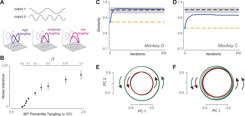
Figure 7.

Leveraging the observation of low tangling to predict the neural population response. A. Illustration of how the same output can be embedded in a larger trajectory with varying degrees of tangling. Top gray traces: A desired two-dimensional output [cos t; sin 2t] Plotted in state space, the output trajectory is a figure eight, and contains a central point that is maximally tangled. Adding a third dimension (βsin t) reduces tangling at that central point. The figure-eight can still be decoded via projection onto two dimensions, in which case the third dimension falls in the null-space of the decode. B. Noise robustness of recurrent networks trained to follow the internal trajectory [cos t; sin 2t; βsin t]. By varying β, we trained multiple networks that could all produce the same figure-eight output, but had varying degrees of trajectory tangling. For each network, noise tolerance was the largest magnitude of state noise for which the network still produced the figure-eight output. For each value of β we trained 20 networks, each with a different random weight initialization. Error bars show the SEM across such networks. C. Similarity of the predicted and empirical motor-cortex population responses (monkey D). Blue trace: prediction yielded by optimizing the cost function in Equation 2. Light blue dot indicates similarity at initialization. Dashed lines show benchmarks as described in the text. Gray shading indicates 95% confidence interval on the upper benchmark, computed across multiple random divisions of the population. D. Same but for monkey C. E. Projection of the predicted population response (after optimization was complete) onto the top two principal components. Data are for monkey D. Green / red traces show trajectories for three cycles of forward / backward cycling respectively. F. Same but for monkey C.