Evaluation of Statistical Inference on Empirical Resting State fMRI

Abstract

Modern statistical inference techniques may be able to improve the sensitivity and specificity of resting state functional magnetic resonance imaging (rs-fMRI) connectivity analysis through more realistic assumptions. In simulation, the advantages of such methods are readily demonstrable. However, quantitative empirical validation remains elusive in vivo as the true connectivity patterns are unknown and noise distributions are challenging to characterize, especially in ultra-high field (e.g., 7T fMRI). Though the physiological characteristics of the fMRI signal are difficult to replicate in controlled phantom studies, it is critical that the performance of statistical techniques be evaluated. The SIMulation EXtrapolation (SIMEX) method has enabled estimation of bias with asymptotically consistent estimators on empirical finite sample data by adding simulated noise [1]. To avoid the requirement of accurate estimation of noise structure, the proposed quantitative evaluation approach leverages the theoretical core of SIMEX to study the properties of inference methods in the face of diminishing data (in contrast to increasing noise). The performance of ordinary and robust inference methods in simulation and empirical rs-fMRI are compared using the proposed quantitative evaluation approach. This study provides a simple, but powerful method for comparing a proxy for inference accuracy using empirical data.

I. Introduction

THE exploration of relational changes within the human brain plays an important role in understanding the brain structure and function, helping with disease prediction and prevention. Neuroscience and patient care have been transformed by quantitative inference of spatial-temporal brain correlations in normal and patient populations with a few millimeters resolution and seconds precision using three-dimensional structural imaging (magnetic resonance imaging—MRI, computed tomography—CT) and functional imaging (positron emission tomography—PET, functional MRI—fMRI) [2]. Classical statistical approaches allow mapping of brain regions associated with planning/execution, response, and default mode behaviors (through task, event, and resting state paradigms, respectively) [3]. When the brain is at rest (i.e., not task driven), functional networks produce correlated low-frequency patterns of activity that can be observed with resting state fMRI (rs-fMRI). These correlations define one measure of functional connectivity which may be estimated by voxel-wise regression of activity in a region of interest (ROI) against that of the remainder of the brain [4]. The selected ROI is called seed. Connectivity analysis has been widely studied using rs-fMRI and seed method analysis [5], [6]. The sensitivity and specificity of connectivity inference techniques hinge upon valid models of the noise in the observed data. Yet, in the quest to evermore specifically map neural anatomy, cognitive function, and potential pathologies, the resolution limitations of the current generation of clinical MRI scanners are becoming painfully clear— especially in imaging of small structures (e.g., [7]). The next generation of 7T MRI scanners offers the possibility of greatly increased signal-to-noise ratio (SNR) along with higher contrast for functional activity [8]. Yet, as the magnetic field strength increases, the effects of physiological noise (breath, local flow, and bulk motion), susceptibility artifacts, and hardware-induced distortion are increased [9]. Hence, artifacts are an increased problem with fMRI at 7T over the current 3T and 1.5T scanners [10].

Absolute voxel-wise MRI intensities (arbitrary values) are rarely used in isolation for inference— rather, the temporal and spatial patterns/correlations of changes over time are of primary interest. Statistical analyses enable inference of the probability that observed signals are not observed by chance (i.e., that there exist significant associations between the observed signals and model of brain activity). The techniques in widespread use are based on classical distributional properties (e.g., Gaussian noise models, autoregressive temporal correlation, and Gaussian random fields) and have been shown to be reasonable for well-designed studies at traditional field strengths. Classical statistics here means least-squares centric approach that lies at the heart of the Statistical Parametric Mapping MATLAB toolbox [11], [12]. Note that for the low SNR, the MRI noise follows a Rician distribution across an image [13], [14], the Rician distribution needs to be well considered to provide unbiased estimation when the temporal SNR is low [15], [16]. But for the rs-fMRI time series observations, the temporal SNR is usually high enough (>3:1~5:1) so that the approximation of the Gaussian distribution assumption is reasonable [13]. The discussion of the ultralow temporal SNR is beyond the scope of this paper. Violations of statistical assumptions threaten to invalidate or (at best) reduce the power of these experiments. Traditional validation guidance involves careful inspection of residuals and evaluation of distributional assumptions [17]. When artifacts are detected, images must be excluded or the analysis approach must be modified. While imaging techniques continue to improve acquisitions in terms of spatial and temporal characteristics (i.e., resolution, signal characteristics, and noise characteristics), it is uncertain if inevitable tradeoffs resulting in altered noise and artifact levels can be controlled or compensated for such that their overall impact will be truly negligible.

The increased ratio of physiological noise to thermal noise [18] may increase the artifacts on 7T fMRI images compared to 3T fMRI. As the prevalence of artifacts increases, the violations of the Gaussian distribution assumptions over all observations underlying the statistical model may also increase. In a recent pilot study, we investigated the distributional properties of rs-fMRI at 3T and 7T [19]. Increasing static field strength from 3T to 7T provides increased signal and contrast, though this increase is commonly traded for improvements in spatial and temporal resolution. As such, the resulting data do not necessarily have the same noise structures, nor are they necessarily well described by traditional Gaussian noise distribution assumptions. In fact, the 7T data presented here exhibited substantial non-Gaussian noise structure and spatial correlations not well modeled by traditional approaches (as would be expected with data known to be susceptible to artifacts) [10]. The statistics literature is ripe with studies demonstrating “robust/resistant” analysis methods that mimic traditional analyses but are less sensitive to the impacts of artifacts and errors in distributional assumptions. For example, a robust empirical Bayesian estimation of longitudinal data is briefly discussed in [20] in a nonimaging context and temporal artifacts have been considered for 3T fMRI by robust estimation of the covariance matrix of the regression errors [21]. We combined these ideas to extend the traditional ReML approach to use a robust autoregressive model. Instead of using ordinary least-squares (OLS) method in coefficients estimation, we used the robust M-estimator estimation to account for the possible outliers. Superior performance was demonstrated in simulation via specificity and sensitivity modeling (e.g., receiver operating characteristic characterization). When applied to empirical 7T fMRI data, clear differences in statistical parameter maps were observed between inferences based on classical and robust assumptions. Yet, there is a fundamental gap between noting empirical differences in statistical parametric maps and concluding that improvement occurred such that one inference method is more appropriate than another. The problem is illustrated on an fMRI dataset with a simulated artifact scan in Fig. 1.

Fig. 1.

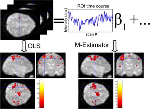
When different inference methods result in different connectivity maps, it is difficult to quantify which is more “valid.” For example, the connectivity of resting state fMRI can be analyzed by fitting region of interest’s (red mark) time course to all activity. A robust method reduces to influence of violations of distributional assumptions (artifacts), but also reduces statistical power. The focus of this study is how to evaluate the statistical parametric maps from different potential analysis approaches.

Statistical comparison of statistical maps (e.g., t-fields, F -fields, p-values) can be theoretically challenging given the difficulty in modeling distributional assumptions when the null hypothesis is rejected [22]. When repeated datasets are available, one can measure the reproducibility of estimated quantities when inference is applied to each dataset separately [23]. Data-driven prediction and reproducibility metrics enable such quantitative assessments through resampling/information theory [24]. Prediction evaluates the degree (e.g., posterior probability) to which a model can assign correct class labels to an independent test set, while reproducibility measures the similarity (correlation coefficient) of activation maps generated from independent datasets. These techniques can be used to optimize acquisition protocols [25] and postprocessing pipelines [26] when true class labels are known. In a related manner, mutual information metrics between the patterns of task activity and image intensity [27] can be used to assess relative predictability and reproducibility characteristics of the robust and classical inference methods. Yet, generalization of these approaches to generic rs-fMRI experimental designs within the general linear model paradigm (i.e., resting state fMRI, structural-functional association studies, etc.) is problematic, and to date, no methods have been proposed to quantify relative performance of rs-fMRI inference methods based on typically acquired datasets (i.e., without large numbers of repeated scans for a single subject).

Herein, we characterize empirical, finite sample performance by quantifying the consistency and resilience of empirical estimators under random data loss (i.e., decimation). These metrics are simple to compute, readily applied to compare estimators of differing types (robust, non-parametric, classical, etc.), and provide metrics that enable data-driven estimator selection. These efforts build on recent innovations in SIMulation and Extrapolation [1] (i.e., SIMEX—the notion that the expected value of an estimator diverges smoothly with increasing noise levels; therefore, the mean degree of corruption can be estimated by extrapolating a trend of divergence when synthetic noise is added to empirical data) and randomized data subsampling. We apply this new technique to characterize ordinary and robust inference of rs-fMRI data. The proposed approach does not require acquisition of additional data and is suitable for evaluation on isolated datasets as well as group datasets.

II. Theory

A. Terminology

For consistency, we adopt the following notation. Scalar quantities are represented by italic, lower case symbols (e.g., σ²). Vectors are represented by bold, italic, lower case symbols (e.g., y). Matrices are bold, upper case symbols (e.g., X). The symbol ~ is used to note “distributed as,” with N used to represent the multivariate Normal distribution. The term “artifacts” refers to unusual observations and the term “noise” is signal not of interest, which may due to physiological or thermal effects. The term “error” refers to the regression error which may or may not contain noise or artifacts.

B. Regression Model

Within this context, we focus on rs-fMRI data, which can be analyzed with an autoregressive model of order 1 (AR(1)) for a weakly stationary time series [28],

$${\mathbf{y}}_i=\mathbf{X}{\beta }_i+e_i,e_i~\mathcal{N}(0,{\sigma }_i^2\mathbf{V})$$ (1)

where y_i is a vector of intensity at voxel i, X is the design matrix containing seed voxel time series, β_i is a vector of regression parameters at voxel i, and e_i is a nonspherical error vector. The correlation matrix V is typically estimated using restricted maximum likelihood (ReML) method with an AR(1) correlation matrix structure, and β is estimated on the whitened data (i.e., the “OLS” approach). Alternatively, a robust estimator (e.g., the “Huber” M-estimator [29]) may be applied after whitening. Both the OLS and Huber methods are available within the SPM software [30]. Herein, we used the Huber method with the tuning constant chosen for 95% asymptotic efficiency when the distribution of observation error is a Gaussian distribution [31].

C. Monte Carlo Assessment of Inference

Empirical characterization of inference performance when the true value is unknown is a circular problem—to quantify error, one must have a baseline against which to compare, but, to compute a baseline from empirical data, one needs an estimator. The SIMEX [1] approach offers a seemingly implausible, but extraordinarily powerful, shortcut around the issue of unknown ground truth. The theoretical core of SIMEX is that the expected value of an estimator diverges smoothly with increasing noise level; therefore, the mean degree of corruption can be estimated by extrapolating a trend of divergence when synthetic noise is added to empirical data [32]. Assuming that the statistical methods under consideration are consistent (i.e., that estimates improve with increasing information), one can use the marginal sensitivity to information loss (e.g., increasing noise) to compute the expected estimator bias based on synthetic noise and a single dataset. SIMEX was developed as a general method that is highly adaptable, which has been extended into classification settings [33] as well as applied in MRI diffusion tensor imaging [34]. In the context of this study, it is not reasonable to add noise because the noise distributions are uncertain—especially in the context of artifacts.

If we apply the SIMEX assumption of smooth convergence to the problem of imaging inference with unknown noise / artifact distributions, we can probe the marginal reduction in sensitivity of an estimator by removing data. We define resilience as the ability of an inference method to maintain a consistent parametric map estimate despite a reduction in data. Over the time course of an rs-fMRI experiment (5–10 mins), the active brain regions vary. Hence, reproducibility of inferences based on sampled time periods (e.g., first versus second half) are not meaningful. Therefore, we focus on diminishing random data samples as opposed to structured temporal resampling. The number of diminished scans is small, and Monte Carlo simulations procedures are used to estimate the mean marginal impact using many different randomly decimated data. Examples of subsampling for one voxel t-value are displayed in Fig. 2.

Fig. 2.

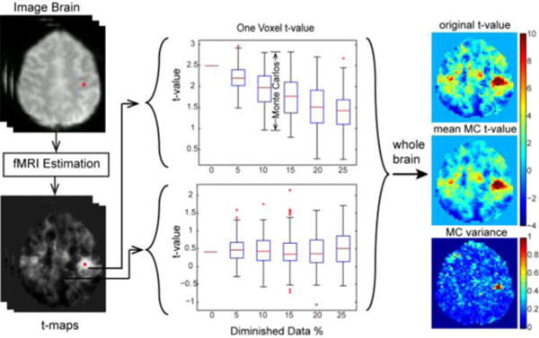
Representative one voxel t-values as data are randomly decimated. An rs-fMRI dataset is randomly diminished into N data size levels with M subsets in each level. Inference methods are applied to each subset to estimate voxel-wise t-maps. The highlighted point (left) indicates the rs-fMRI seed region.

The scans are randomly deleted after all preprocessing steps so that the changes of scan intervals do not affect the slice timing correction or low-pass filtering. Recall that the temporal covariance of fMRI time series is estimated using ReML with an AR(1) correlation structure. To address the scan interval changes, we modified the temporal correlation matrix according to the number of time points between every two image. In SPM, low-frequency confounds are removed before estimation using residual formatting matrix. To address random data removal, we generated the low-frequency filtering matrix for the whole data then deleted the time points corresponding to the scans removed.

D. Resilience

An intuitive way to assess the resilience of an inference method to a reduction in data might be to calculate the absolute value of the difference between the mean t-values (across Monte Carlo simulations) as a function of data size. However, this method will result in higher difference when the t-value with all data is high versus the t-value with all data is low as data reduction will universally pull t-values away from significance. Such an approach will strongly depend on the true effect size and the mean t-value cannot reflect the resilience to the artifacts if any [35]. Hence, it is important to also consider the variance of the estimated parametric maps—we advocate evaluating the resilience in terms of consistency and variance.

Small reductions in data result in approximately linear reductions in t-value (due to smooth loss of power–not shown), so we advocate focusing on a specified diminished data size (e.g., randomly diminished by 10% and 20%) rather than on a large number of different data decimations. At a single data size with 10% decimation, we have three parametric maps of data across all spatial locations; one t-map of the starting t-values, one t-map of the mean t-value from the Monte Carlo repetitions, and one variance map from the Monte Carlo repetitions. The right subplots in Fig. 2 show one slice of the t-map fields with the mean and the variance of the t-value over the subsamples.

Consistency assesses the bias of the computed parametric map of the decimated data relative to the same map computed with complete data. A priori, one would expect to see small reductions in parametric map values between the complete and decimated datasets due to the power loss, but there would be few large changes as both classical and robust inference methods are reasonably unbiased. We summarize consistency by pooling information across all in-brain voxels using linear regression:

$${\mathbf{t}}_{\overline{MC}}={\beta }_{\text{mean}}\times {\mathbf{t}}_{\text{all}}+\mathbf{\epsilon }$$

$$r_{\text{con}}={\beta }_{\text{mean}}-1$$ (2)

where t_all is a vector containing one t-value for each in-brain voxel, where the t-value is estimated using the overall time series, $t_{\overline{MC}}$ is the mean t-value of all subsamples (across Monte Carlo iteration), and the slope β_mean reflects the pooled consistency (see Fig. 3). If the inference method is consistent, β_mean should be close to one and the fitting error would be small. The value of r_con can therefore be viewed as a reflection of bias with the sign indicating positive or negative bias and the R-squared can assess the goodness of fit relative to the random error (ε). As we are losing data, we can expect lower t-values for significant voxels, thus β_mean will not equal one but should be close to one. Hence, a statistical test is not appropriate—we know the true distributions are different—rather, we must use the numerical value of β_meanin a qualitative assessment.

Fig. 3.

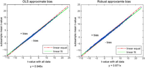
Illustration of consistency estimation. The mean t-value of random subsamples with 10% diminished data (vertical) is plotted versus the t-value with all data (horizontal). The left plot displays the OLS estimates and the right shows the M -estimates. The dashed line indicates equality (y = x); the data points above the dashed line have positive bias and the points below the dashed line have negative bias. The solid line is the estimated regression line from all the data points in each plot.

The variance of the t-values across Monte Carlo samples for a diminished data size can reflect how resistant an estimation method is to artifacts in the dataset. If a method is affected by artifacts, the variance will increase when artifacts exist. This is because the artifacts may appear in some subsamples while not in others which will result in varied t-value estimates. Although the inference method with overall smaller variances is more resistant to artifacts, the artifacts may exist only in some brain regions. These regional effects are difficult to detect from looking directly at a variance map as in Fig. 2. To account for the influence of regional or a small number of artifacts, the variances from two inference methods are compared directly (see Fig. 4). The collection of variance values across spatial locations for inference method-1, var1_MC, (e.g., OLS) is plotted against those of inference method-2, var2_MC, (e.g., robust) and their variances are compared by computing the slope β_var between them under consideration of random error (ε).

$$\mathit{\text{var}}{\mathbf{2}}_{MC}={\beta }_{\mathit{\text{var}}}\times \mathit{\text{var}}{\mathbf{1}}_{MC}+\mathbf{\epsilon }$$ (3)

Fig. 4.

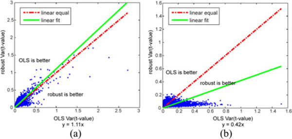
t-value variance comparison. The variance of subsample t-values with 10% diminished data from OLS (horizontal) and robust estimation (vertical) methods are compared. The dashed line (y = x) shows when the variance from the OLS and robust method are equal. The solid line is the estimated regression line.

If these two methods are equivalent, the slope will be close to 1. If the slope is larger than 1, the method-1 is superior; on the contrary, if the slope is smaller than 1, the method-2 is superior. The slope is impacted when one method contains spatial locations with larger variance which may due to the impact of artifacts. Fig. 4 displays two examples, and Fig. 5 presents corresponding brain images indicating the spatial locations where the variance from robust estimation is lower than the variance from OLS.

Fig. 5.

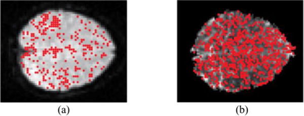
t-value variance comparison corresponding brain images. The red points represent where variance from robust estimation that is lower than the variance from OLS. (a) corresponds to Fig. 4(a) and (b) corresponds to Fig. 4(b).

When using robust regression, we have to pay the price that it is 95% asymptotically Gaussian when there are no artifacts (i.e., 5% reduction in power). To compare the OLS and robust variance, we selected the variance from OLS as var1_MC and the variance from Huber estimation as var2_MC in (3), if the slope is less than 1, the robust estimation is practically superior to OLS estimation.

III. Methods and Results

A. Simulation Experiments

1) Simulation Data

To investigate the properties of our method in a controlled environment, we first performed simulation experiments. In the simulation, a simple regression model is used:

$${\mathbf{y}}_{\mathbf{\text{obs}}}={\beta }_0+{\mathbf{x}}_{\mathbf{\text{obs}}}\times {\beta }_1+e,e~N(0,{\sigma }^2\mathbf{V})$$ (4)

where x_obs simulates the seed voxel time course, β₁ is the connectivity coefficient, and V is the normalized covariance matrix. x_obs is acquired from an empirical 3T unsmoothed fMRI data. (The source fMRI data are preprocessed through slice timing correction, realignment, and normalized to Talairach space.) We selected a voxel inside the right motor cortex and acquired its time series. The time series was demeaned to simulate the value of x_obs. The mean value of the original (un-demeaned) voxel time course is about 905 (arbitrary intensity units), and the standard deviation is about 11. So, we designed the simulated temporal signal-to-noise ratio (TSNR) to be 80:1 (≈905/11). We used β₁ = 0.8 for other voxels (β₁ = 1 for the seed voxel) inside the right side of gray matter (GM), β₁ = −0.6 for the voxels inside the left side of GM, and β₁ = 0 for the rest of the brain. The mean value of a white matter voxel time course is about 800 so β₀ is set to make the whole brain mean value to be around 800. We calculated y_true based on these parameters.

$${\mathbf{y}}_{\mathbf{\text{true}}}={\beta }_0+{\mathbf{x}}_{\mathbf{\text{obs}}}\times {\beta }_1.$$ (5)

For each voxel, we generated Gaussian noise N (0, σ²I) for the first time point, and then convolved the Gaussian noise to generate autoregressive noise with correlation 0.2 across time. σ is chosen to make TSNR ≃ 80:1. We added the autoregressive noise to y_true to simulate fMRI images. In this simulation, the AR(1) parameter is constant for all voxels, but the estimation method does not estimate the AR(1) parameter, instead, it estimates the covariance matrix of the temporal noise [36]. The seed voxel time course is considered as the design matrix.

To simulate artifacts, we created an outlier scan by adding Gaussian noise with higher standard deviation to a simulated scan. The outlier scan is chosen with the highest seed intensity and the noise is only added to a region of the brain. The added Gaussian noise is zero mean with standard deviation 10 times the standard deviation of the original simulated scan. Other simulated scans are kept the same.

2) Subsample Parameters and Simulation Results

User controlled parameters for implementing our method include 1) the number of Monte Carlo simulations and 2) the diminished data size. To decide the number of Monte Carlo simulation and the diminished data size, we evaluate their influence on the consistency and the variance on simulation data as shown in Fig. 6. To decide the number of Monte Carlo simulations, we plotted the r_con for the OLS consistency (2) and 1 − β_var for the variance comparison (3). Plots were made for two variance comparison across five similar simulations when 10% of scans are randomly diminished. When there is only one Monte Carlo simulation, the range of the boxplot is large and it decreases as the number of Monte Carlo simulations increase.

Fig. 6.

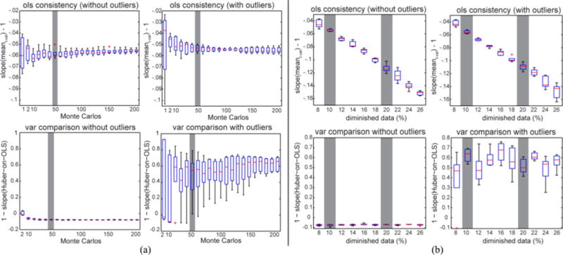
Influence of resilience parameter. (a) shows the impact of the number of Monte Carlo repetitions with 10% diminished data. (b) shows the impact of the diminished data size level when we performed 50 Monte Carlos each time. The OLS consistency plots display the slope β_mean − 1 in (2). The variance comparison plots display 1 − β_var, where β_var is the slope of variance from robust estimation on OLS. “With\without artifacts” indicates if there are simulated outlier scans in the simulation.

The consistency from the OLS and the robust (not shown in the figure) inference are similar with and without outliers if the number of Monte Carlo simulations is over 50. When there are no outliers, the variance slope β_var is greater than 1, which suggests that the OLS method is better than the robust method. When there are outliers, β_var is less than 1, which suggests that the robust method is better than the OLS method.

B. Empirical Experiments

1) Empirical Data

For illustrative purposes, we consider two distinct in vivo datasets.

Rs-fMRI acquired at 3T was downloaded from http://www.nitrc.org/projects/nyu_trt/ with 25 healthy subjects each scanned in three sessions providing 75 rs-fMRI time series in total (197 volumes, FOV = 192 mm, flip θ = 90°, TR/TE = 2000/25 ms, 3 × 3 × 3 mm, 64 × 64 × 39 voxels) [37]. Prior to analysis, all images were corrected for slice timing artifacts, corrected for motion artifacts, nonlinear spatially normalized to MNI space, and spatially smoothed with an 8 mm FWHM Gaussian kernel using SPM8 (University College London, U.K.). All time courses were low-pass filtered at 0.1 Hz using a Chebychev Type II filter, linearly detrended, and demeaned. The 3T data are smoothed, a typical preprocessing step for 3T fMRI to increase spatial SNR. Two voxels inside the right primary motor cortex for each subject were manually selected as the region of interest (ROI) by experienced researchers through exploring the unsmoothed images and comparing with the standard atlas. The design matrix for the general linear model was defined as the ROI time courses, the six estimated motion parameters, and one intercept. To create whole-brain connectivity maps, every labeled brain voxel underwent linear regression using the design matrix.

Eight normal subjects were studied at 7T after informed consent. Subjects were instructed to both close their eyes and rest. Briefly, the resting state images were acquired for 500 s using single shot gradient echo EPI (500 volumes, FOV = 192 mm, flip θ = 53.8°, TR/TE = 1000/28 ms, SENSE factor = 3.92, no partial read out or phase encoding, resolution 2 × 2 × 2 mm, 96 × 96 × 13 voxels). Please see [38] for a discussion of the impacts of parallel imaging on noise characteristics. Prior to analysis, all images were corrected for slice timing artifacts and motion artifacts using SPM8 (University College London, UK). All voxels’ time courses were low-pass filtered at 0.1 Hz using a Chebychev Type II filter, linearly detrended, and demeaned. The 7T data are not smoothed because the spatial SNR are much higher in 7T than 3T, and we are only interested in single subject results that smoothness is not necessary. The seed voxel was defined as a single manually selected voxel located in primary motor cortex along the central sulcus that was also significantly activated by a conventional finger tapping task contrasting bimanual, self-paced finger tapping against a resting condition (FWE corrected, p < 0.05, minimum cluster size = 1 voxel) [39]. The design matrix for the general linear model was defined as the seed voxel time course, the six estimated motion parameters and the intercept. Each voxel’s BOLD time course underwent linear regression of the design matrix to create connectivity maps.

2) Comparative Analysis of Classical and Robust Inference

rs-fMRI analysis was performed on each dataset in SPM8 using ordinary “OLS” and robust (“Huber”) regression methods. For each decimation level (10% and 20%), 50 Monte Carlo simulations were performed. For each Monte Carlo simulation, a subset of either 90% or 80% of the total data was randomly selected, the OLS and Huber estimation methods were applied, and the t-maps on the coefficient for the ROI time courses were stored. Consistency was assessed between the mean of the decimated maps and the map using all data, while the relative variance was assessed between Monte Carlo simulations with each method. For the resilience variance metrics, OLS was on the x-axis and Huber on the y-axis. Note that both OLS and Huber were fit to the same subsample of the data (i.e., the random subsamples are paired).

3) Empirical Results

Representative statistical parametric maps from OLS and robust regression of one 3T fMRI and two 7T fMRI are displayed in Fig. 7. Noted that the results are shown on uncorrected p-value without cluster size threshold, the difference between results from OLS and robust regression may be more obvious than the results after cluster threshold. The results of all subjects are displayed in Fig. 8 and summarized in Table I (and detailed in supplementary material). Next, we discuss how the qualitative metrics may be used for selection of the inference method.

Fig. 7.

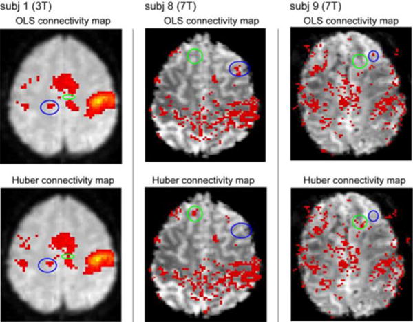
Representative overlays significant for three subjects (columns) with OLS (top row) and robust (lower row) estimation methods. The connectivity maps are computed from one-sided t-test on the ROI time course coefficients (p < 0.001, uncorrected). The blue circle shows that the OLS result is significant, while the robust result is not or less significant. The green circle shows that the robust result is significant while the OLS result is not or less significant. Resilience measures are tabulated in TABLE I.

Fig. 8.

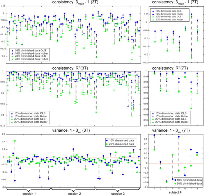
Empirical results. The left column shows the results of 3T data with 25 subjects each has 3 sessions. The right column shows the results of 7T data with 8 subjects. The top and the middle rows show the consistency results. The top row displays the slope β_mean − 1, and the middle row displays the goodness of fit R². The circle represents the value from OLS estimation, the triangle represents the value from Huber estimation, the plots in blue are from 10% diminished data size, and the plots in green are from 20% diminished data size. Results from the same subject in the same session are linked with the black-dashed line. The bottom row shows the variance results. The blue dots represent the results from 10% diminished data size and the green dots represent the results from 20% diminished data size. The red line displays the position where the performance of OLS and the Huber estimation are equal.

TABLE I.

Summary of Resilience Measures for all Subjects

	3T (proportion)	7T (proportion)
(1 −βvar)<0 for 10% and 20% diminished data	53/75	2/8
(1 −βvar)<0 for 10% diminished data (1 −βvar)>0 for 20% diminished data	10/75	1/8
(1 −βvar)>0 for 10% diminished data (1 −βvar)<0 for 20% diminished data	8/75	3/8
(1 −βvar)>0 for 10% and 20% diminished data	4/75	2/8

1. For 53 3T and 2 7T rs-fMRIs, the consistency estimates are similar and close to zero for both OLS and Huber, while the R-squared value is high. This indicates that neither method is particularly biased by the decimation process. The variance matrices for both 10% and 20% decimation are negative, which indicates that OLS was more resilient than Huber.

   Conclusion: Robust inference is not necessary; OLS is preferable. When there are no outliers, the OLS method is better than the robust method because the robust method is only approximately 95% as statistically efficient as the OLS method. The evaluation conclusion indicates that there are relatively few outliers in this dataset.

2. For 4 3T and 2 7T rs-fMRIs, the consistency estimates are similar and close to zero for both OLS and Huber, and the R-squared value is high. Hence, neither method is particularly biased by the decimation process. The variance metric for both 10% and 20% decimation is positive, which indicates that Huber was more resilient than OLS.

   Conclusion: Robust inference yields higher resilience and should be used. It indicates that there are outliers in this data set. Since the probability of the existence of outliers increase at 7T compared to 3T it is not surprising that the robust inference method is better than the OLS.

3. For 18 3T and 4 7T rs-fMRIs, the consistency estimates are similar and close to zero for both OLS and Huber, and the R-squared value is high. Hence, neither method is particularly biased by the decimation process. The biases at 20% decimation are always higher and the R-squared value is lower than at 10% decimation for all these subjects. For 10 3T and 1 7T fs-fMRIs, the variance metric for the 10% decimation is negative, while the variance metric for the 20% decimation is positive. For 8 3T and 3 7T rs-fMRIs, the variance metric for the 10% decimation is marginally positive while the variance metric for the 20% decimation is negative. The mixed results indicate that neither method is clearly superior and that careful data inspection is warranted.

   Conclusion: Robust inference may be desirable, but OLS could be suitable. The similar performance of the robust and the OLS methods may due to the fact that there are outliers but the number is small. In that situation, the OLS is better in most brain regions but the robust inference is much better in some small regions. Both methods yield acceptable results.

IV. Discussion and Conclusion

The proposed resilience metrics provide a quantitative basis on which to compare inference methods. The simulation results suggest that a comparison of methods based on resilience would yield similar conclusions as one based on the sensitivity and specificity matrix. Yet, resilience is accessible for empirical data, whereas the ground truth (necessary for sensitivity and specificity) is rarely known. In our empirical study, the resilience indicates that OLS would outperform the robust inference approach on most 3T dataset, while the robust approach would outperform OLS on higher portion of the 7T dataset. This is consistent with our knowledge that the propensity for artifacts increases in 7T since the achievable SNR increases. Another reason of this finding may be the 3T data were smoothed that would be more normally distributed than the 7T data which were not smoothed. Smoothness can make the data more normally distributed, but will blur the images and introduce more spatial correlations. The 7T data were not smoothed because the SNR has been found to be high enough for detection. The robust estimation also assumes asymptotic Gaussian distribution but accounting for the possibility of outliers, and it outperforms OLS when outliers occur in Gaussian distributed data. The comparison of OLS and robust estimation on data following other distributions may need further study but beyond the scope of this paper.

In simulations, it is easy to construct realistic datasets demonstrating that classical assumptions are sufficient or insufficient. However, in reality, it is very difficult to assess the stability of the robust/nonrobust decision to variations in artifacts. Hence, creating representative artifact-prone distributions is a substantial endeavor. It is possible to acquire a massive reproducibility dataset and use this dataset to produce a highly robust ground truth estimate. Given such data, one may map artifact distributions. However, such acquisitions are exceedingly resource intensive and may not be representative of other sites and/or acquisitions. Hence, generalization of artifact findings is problematic.

However, the proposed resilience consistency and variance metrics provide a quantitative basis on which to judge individual datasets, allowing one to evaluate suitability of particular inference mechanisms on initial pilot data. This could be done in case studies, or as part of multilevel analysis to evaluate the tradeoffs between improved power (when classical assumptions are met) and reduced susceptibility to artifacts, based on actual empirical data.

Consistency in statistics is defined as convergence in probability, i.e., a consistent estimator of parameter converges to its true value as sample size grows. However, in practice it is not feasible to prove the consistency of an estimator because the truth remains unknown. What we assessed in this paper is not the absolute consistency but rather the relative consistency as it related to resilience of an estimator, which could be achieved when estimated values were relatively stable regardless of the amount of data used as illustrated in Section II. We are not intending to empirically prove that the robust estimator is an absolutely consistent, but we want to show that estimates based on the robust estimator can be more (or less) consistent (or invariable) than another as decimated data are utilized.

Generally, the evaluation result depends on the number of effective outliers in the brain. In some cases, the evaluation is location dependent such that one estimator is good for one seed but not good for another, especially when outliers exist in one region but not in others. The resilience method still can be used to evaluate inference methods (e.g., see Fig. 5), albeit without the increased power gained by pooling regions.

The random decimation procedure can be problematic for aspects of temporal estimation. We initially sought to examine split half (either temporal: early/late or frequency: even/odd). Unfortunately, both lead to systematic differences in the quantities being estimated by rs-fMRI. Temporal subsampling dramatically reduces the sensitivity to low-frequency correlations (which are of primary interest) and focuses analysis on short time periods with potentially different biological states. Frequency subsampling reduces the intrinsic sensitivity to temporal frequencies and imparts differing sensitivity to artifact. We examined a number of different random decimation methods and propose random decimation as a compromise between empirical power (i.e., we see differences where ones are known to exist) and ease of use.

Implementation of this approach requires the ability to decimate (remove) data randomly, loop over multiple possible data subsets, and calculate summary measures of the resulting statistical fields. With modern multi-core and cluster environments, a 50–100 fold increases in the computational burden of a traditional analysis is not typically problematic for offline analysis. For example, the experiments presents that one OLS analysis takes approximately 40 s and one Huber analysis takes 100 min. With proper parallelization, the total wait time would not be substantively longer than the time for a single analysis.

In conclusion, we have presented a novel approach for quantifying inference methods based on empirical data. We evaluated the resilience of the ordinary (OLS) and a robust method for both simulated and empirical data. Resilience provides a simple, but powerful method for comparing a proxy for accuracy of inference approaches in empirical data where the underlying true value is unknown. Statistical theories characterizing finite sample statistical behavior are undergoing rapid and exciting developments in the statistical community. These statistical methods, encompassing SIMEX, bootstrap, and Monte Carlo approaches, offer the potential to understand both the uncertainty and bias in metrics estimated from imaging data. Given the abundance of computational power generally available, these methods can now be feasibly applied on routine basis.

References

- 1.Carroll RJ, Ruppert D, Stefanski LA, Crainiceanu C. Measurement Error in Nonlinear Models: A Modern Perspective. Vol. 105 Boca Raton, FL, USA: CRC Press; 2006. [Google Scholar]
- 2.Matthews PM, Honey GD, Bullmore ET. Applications of fMRI in translational medicine and clinical practice. Nat Rev Neurosci. 2006;7:732–744. doi: 10.1038/nrn1929. [DOI] [PubMed] [Google Scholar]
- 3.Penny WD, Friston KJ, Ashburner JT, Stefan JK, Nicholas TE. Statistical Parametric Mapping: The Analysis of Functional Brain Images. New York, NY, USA: Academic; 2007. [Google Scholar]
- 4.Van Den Heuvel MP, Hulshoff Pol HE. Exploring the brain network: A review on resting-state fMRI functional connectivity. Eur Neuropsychopharmacol. 2010;20:519–534. doi: 10.1016/j.euroneuro.2010.03.008. [DOI] [PubMed] [Google Scholar]
- 5.Biswal B, Zerrin Yetkin F, Haughton VM, Hyde JS. Functional connectivity in the motor cortex of resting human brain using echo-planar MRI. Magn Resonance Med. 1995;34:537–541. doi: 10.1002/mrm.1910340409. [DOI] [PubMed] [Google Scholar]
- 6.Bandettini PA, Jesmanowicz A, Wong EC, Hyde JS. Processing strategies for time-course data sets in functional MRI of the human brain. Magn Resonance Med. 1993;30:161–173. doi: 10.1002/mrm.1910300204. [DOI] [PubMed] [Google Scholar]
- 7.Giove F, Garreffa G, Giulietti G, Mangia S, Colonnese C, Maraviglia B. Issues about the fMRI of the human spinal cord. Magn Reson Imag. 2004 Dec;22:1505–1516. doi: 10.1016/j.mri.2004.10.015. [DOI] [PubMed] [Google Scholar]
- 8.Hutchison RM, Leung LS, Mirsattari SM, Gati JS, Menon RS, Everling S. Resting-state networks in the macaque at 7T. Neuroimage. 2011;56:1546–1555. doi: 10.1016/j.neuroimage.2011.02.063. [DOI] [PubMed] [Google Scholar]
- 9.Hutton C, Josephs O, Stadler J, Featherstone E, Reid A, Speck O, Bernarding J, Weiskopf N. The impact of physiological noise correction on fMRI at 7T. Neuroimage. 2011;57:101–112. doi: 10.1016/j.neuroimage.2011.04.018. [DOI] [PMC free article] [PubMed] [Google Scholar]
- 10.Triantafyllou C, Hoge R, Krueger G, Wiggins C, Potthast A, Wiggins G, Wald L. Comparison of physiological noise at 1.5T, 3T and 7T and optimization of fMRI acquisition parameters. Neuroimage. 2005;26:243–250. doi: 10.1016/j.neuroimage.2005.01.007. [DOI] [PubMed] [Google Scholar]
- 11.Friston K, Jezzard P, Turner R. Analysis of functional MRI time-series. Human Brain Map. 1994;1:153–171. [Google Scholar]
- 12.Friston KJ, Holmes AP, Poline J, Grasby P, Williams S, Frackowiak RS, Turner R. Analysis of fMRI time-series revisited. NeuroImage. 1995;2:45–53. doi: 10.1006/nimg.1995.1007. [DOI] [PubMed] [Google Scholar]
- 13.Gudbjartsson H, Patz S. The Rician distribution of noisy MRI data. Magn Reson Med. 1995 Dec;34:910–914. doi: 10.1002/mrm.1910340618. [DOI] [PMC free article] [PubMed] [Google Scholar]
- 14.Wink AM, Roerdink JBTM. BOLD noise assumptions in fMRI. Int J Biomed Imag. 2006;2006 doi: 10.1155/IJBI/2006/12014. [DOI] [PMC free article] [PubMed] [Google Scholar]
- 15.Rowe DB. Parameter estimation in the magnitude-only and complex-valued fMRI data models. NeuroImage. 2005;25:1124–1132. doi: 10.1016/j.neuroimage.2004.12.048. [DOI] [PubMed] [Google Scholar]
- 16.Zhu H, Li Y, Ibrahim JG, Shi X, An H, Chen Y, Gao W, Lin W, Rowe DB, Peterson BS. Regression models for identifying noise sources in magnetic resonance images. J Amer Statis Assoc. 2009;104:623–637. doi: 10.1198/jasa.2009.0029. [DOI] [PMC free article] [PubMed] [Google Scholar]
- 17.Luo WL, Nichols TE. Diagnosis and exploration of massively univariate neuroimaging models. NeuroImage. 2003;19:1014–1032. doi: 10.1016/s1053-8119(03)00149-6. [DOI] [PubMed] [Google Scholar]
- 18.Krüger G, Glover GH. Physiological noise in oxygenation-sensitive magnetic resonance imaging. Magn Reson Med. 2001;46:631–637. doi: 10.1002/mrm.1240. [DOI] [PubMed] [Google Scholar]
- 19.Yang X, Holmes MJ, Newton AT, Morgan VL, Landman BA. SPIE Med Imag. San Diego, CA, USA: 2012. A comparison of distributional considerations with statistical analysis of resting state fMRI at 3T and 7T. [DOI] [PMC free article] [PubMed] [Google Scholar]
- 20.Gill PS. A robust mixed linear model analysis for longitudinal data. Statist Med. 2000;19:975–987. doi: 10.1002/(sici)1097-0258(20000415)19:7<975::aid-sim381>3.0.co;2-9. [DOI] [PubMed] [Google Scholar]
- 21.Diedrichsen J, Shadmehr R. Detecting and adjusting for artifacts in fMRI time series data. Neuroimage. 2005 Sep;27:624–634. doi: 10.1016/j.neuroimage.2005.04.039. [DOI] [PMC free article] [PubMed] [Google Scholar]
- 22.Garrett M, Holmes H, Nolte F. Selective buffered charcoal-yeast extract medium for isolation of nocardiae from mixed cultures. J Clin Microbiol. 1992;30:1891–1892. doi: 10.1128/jcm.30.7.1891-1892.1992. [DOI] [PMC free article] [PubMed] [Google Scholar]
- 23.Genovese CR, Noll DC, Eddy WF. Estimating test-retest reliability in functional MR imaging I: Statistical methodology. Magn Reson Med. 1997;38:497–507. doi: 10.1002/mrm.1910380319. [DOI] [PubMed] [Google Scholar]
- 24.Strother SC, Anderson J, Hansen LK, Kjems U, Kustra R, Sidtis J, Frutiger S, Muley S, LaConte S, Rottenberg D. The quantitative evaluation of functional neuroimaging experiments: The NPAIRS data analysis framework. NeuroImage. 2002;15:747–771. doi: 10.1006/nimg.2001.1034. [DOI] [PubMed] [Google Scholar]
- 25.LaConte S, Anderson J, Muley S, Ashe J, Frutiger S, Rehm K, Hansen LK, Yacoub E, Hu X, Rottenberg D. The evaluation of preprocessing choices in single-subject BOLD fMRI using NPAIRS performance metrics. NeuroImage. 2003;18:10–27. doi: 10.1006/nimg.2002.1300. [DOI] [PubMed] [Google Scholar]
- 26.Strother S, La Conte S, Kai Hansen L, Anderson J, Zhang J, Pulapura S, Rottenberg D. Optimizing the fMRI data-processing pipeline using prediction and reproducibility performance metrics—Part I: A preliminary group analysis. NeuroImage. 2004;23:S196–S207. doi: 10.1016/j.neuroimage.2004.07.022. [DOI] [PubMed] [Google Scholar]
- 27.Afshin-Pour B, Soltanian-Zadeh H, Hossein-Zadeh GA, Grady CL, Strother SC. A mutual information-based metric for evaluation of fMRI data-processing approaches. Human Brain Map. 2011;32:699–715. doi: 10.1002/hbm.21057. [DOI] [PMC free article] [PubMed] [Google Scholar]
- 28.Friston KJ, Penny W, Phillips C, Kiebel S, Hinton G, Ashburner J. Classical and Bayesian inference in neuroimaging: Theory. NeuroImage. 2002;16:465–483. doi: 10.1006/nimg.2002.1090. [DOI] [PubMed] [Google Scholar]
- 29.Huber PJ, Ronchetti E, MyiLibrary . Robust Statistics. Vol. 1. New York, NY: Wiley Online Library; 1981. [Google Scholar]
- 30.Yang X, Beason-Held L, Resnick SM, Landman BA. Biological parametric mapping with robust and non-parametric statistics. Neuroimage. 2011 Jul 15;57:423–430. doi: 10.1016/j.neuroimage.2011.04.046. [DOI] [PMC free article] [PubMed] [Google Scholar]
- 31.Holland PW, Welsch RE. Robust regression using iteratively reweighted least-squares. Commun Statist-Theory Methods. 1977;6:813–827. [Google Scholar]
- 32.Cook JR, Stefanski LA. Simulation-extrapolation estimation in parametric measurement error models. J Amer Statist Assoc. 1994;89:1314–1328. [Google Scholar]
- 33.Küchenhoff H, Mwalili SM, Lesaffre E. A general method for dealing with misclassification in regression: The misclassification SIMEX. Biometrics. 2006;62:85–96. doi: 10.1111/j.1541-0420.2005.00396.x. [DOI] [PubMed] [Google Scholar]
- 34.Lauzon CB, Crainiceanu C, Caffo BC, Landman BA. Assessment of bias in experimentally measured diffusion tensor imaging parameters using SIMEX. Magn Reson Med. 2012 doi: 10.1002/mrm.24324. [DOI] [PMC free article] [PubMed] [Google Scholar]
- 35.Yang X, Kang H, Newton A, Landman B. Quantitative evaluation of statistical inference in resting state functional MRI; presented at the Medical Image Computing and Computer-Assisted Intervention; Nice, France. 2012. [DOI] [PMC free article] [PubMed] [Google Scholar]
- 36.Worsley K, Liao C, Aston J, Petre V, Duncan G, Morales F, Evans A. A general statistical analysis for fMRI data. NeuroImage. 2002;15:1–15. doi: 10.1006/nimg.2001.0933. [DOI] [PubMed] [Google Scholar]
- 37.Shehzad Z, Kelly AMC, Reiss PT, Gee DG, Gotimer K, Uddin LQ, Lee SH, Margulies DS, Roy AK, Biswal BB. The resting brain: Unconstrained yet reliable. Cerebral Cortex. 2009;19:2209–2229. doi: 10.1093/cercor/bhn256. [DOI] [PMC free article] [PubMed] [Google Scholar]
- 38.Dietrich O, Raya JG, Reeder SB, Ingrisch M, Reiser MF, Schoenberg SO. Influence of multichannel combination, parallel imaging and other reconstruction techniques on MRI noise characteristics. Magn Reson Imag. 2008;26:754–762. doi: 10.1016/j.mri.2008.02.001. [DOI] [PubMed] [Google Scholar]
- 39.Newton AT, Rogers BP, Gore JC, Morgan VL. Improving measurement of functional connectivity through decreasing partial volume effects at 7T. NeuroImage. 2012;59:2511–2517. doi: 10.1016/j.neuroimage.2011.08.096. [DOI] [PMC free article] [PubMed] [Google Scholar]
Associated Data
This section collects any data citations, data availability statements, or supplementary materials included in this article.