TADs are 3D structural units of higher-order chromosome organization in Drosophila

Drosophila chromosomes are organized in a series of nanocompartments that correspond to topologically associating domains.

Abstract

Deciphering the rules of genome folding in the cell nucleus is essential to understand its functions. Recent chromosome conformation capture (Hi-C) studies have revealed that the genome is partitioned into topologically associating domains (TADs), which demarcate functional epigenetic domains defined by combinations of specific chromatin marks. However, whether TADs are true physical units in each cell nucleus or whether they reflect statistical frequencies of measured interactions within cell populations is unclear. Using a combination of Hi-C, three-dimensional (3D) fluorescent in situ hybridization, super-resolution microscopy, and polymer modeling, we provide an integrative view of chromatin folding in Drosophila. We observed that repressed TADs form a succession of discrete nanocompartments, interspersed by less condensed active regions. Single-cell analysis revealed a consistent TAD-based physical compartmentalization of the chromatin fiber, with some degree of heterogeneity in intra-TAD conformations and in cis and trans inter-TAD contact events. These results indicate that TADs are fundamental 3D genome units that engage in dynamic higher-order inter-TAD connections. This domain-based architecture is likely to play a major role in regulatory transactions during DNA-dependent processes.

INTRODUCTION

The three-dimensional (3D) organization of the genome is closely related to the control of transcriptional programs (1). Recently, high-throughput variants of the chromosome conformation capture method (Hi-C) (2) have been extensively used to molecularly address the 3D spatial organization of genomes [see Bonev and Cavalli (1) for review]. A key architectural feature revealed by Hi-C was the existence of topologically associating domains (TADs) (3–6), corresponding to domains of highly interacting chromatin, with reduced interactions spanning borders between them. In Drosophila, TADs correlate well with functional epigenetic domains defined by chromatin marks (4, 6–8). In mammals, an additional level of TAD organization involves dynamic cohesin-dependent loops between CTCF binding sites at convergent orientations (9–13). The correlation of TAD structures with epigenetic marks can be observed in mammals using high-resolution Hi-C maps (7, 11). This compartmentalization, defined by the underlying chromatin state, appears to be reinforced upon removal of CTCF/cohesin loop components (10, 12, 13), suggesting a conserved mode of chromatin organization across species (7). TADs have been proposed to constrain gene regulation (5, 14), for example, by spatially defining the limits of where an enhancer can act (15, 16). However, this model requires TADs to be physical units when they could instead reflect a statistical feature that emerges when populations of nuclei are analyzed. Recent single-cell Hi-C studies (17–19) showed somewhat contrasting results in this respect. Although one study is compatible with the presence of TADs in individual nuclei (18), another suggests that TADs might reflect a statistical property that appears when individual cells are merged (17). Thus, to what extent the compartmentalization of chromatin into TADs is present in each cell nucleus is still unclear. Furthermore, the relation between TADs and higher-order chromosome folding remains to be explored. Recently, super-resolution microscopy has allowed finer-scale chromatin architecture to be analyzed at the single-cell level (20–22), suggesting that different types of chromatin are characterized by distinct degrees of compaction (23) and opening the possibility of studying the structural properties of chromosome domains.

RESULTS

Chromatin is organized in a series of discrete 3D nanocompartments

To investigate the nature of TADs in single cells, we used Oligopaint (24) and fluorescent in situ hybridization (FISH) to homogenously label an extended 3–million base pair (Mbp) region of Drosophila chromosome 2L (table S1) and imaged its nuclear organization using 3D-structured illumination microscopy (3D-SIM) (25, 26). This region comprises three main types of Drosophila epigenetic domains: active chromatin (Red) enriched in trimethylation of histone 3 lysine 4 (H3K4me3), H3K36me3, and acetylated histones; Polycomb group (PcG) protein repressed domains (Blue), defined by the presence of PcG proteins and H3K27me3; and inactive domains (Black), which are not enriched in specific epigenetic components (Fig. 1A) (6). Although conventional wide-field (WF) microscopy imaging of this region did not reveal internal structures, 3D-SIM showed that this chromosomal region appears as a semicontinuous sequence of discrete globular structures, defined here as nanocompartments (Fig. 1, B to D, and fig. S1, A and B). These structures are interspersed by less intense gap regions despite uniform probe coverage across the 3 Mb (fig. S1C). In addition, the 3-Mb probe intensity variation displayed correlation with whole nucleus staining [4′,6-diamidino-2-phenylindole (DAPI); fig. S1, D to F]. We reasoned that these nanocompartments may reflect the presence of TADs, so we adapted the Oligopaint strategy to two-color chromatin labeling (see Materials and Methods and fig. S2, A and B), simultaneously visualizing the 3-Mb region and single TADs within it (Fig. 1E and table S1). We observed that repressed TADs (Blue and Black) form globular structures that coincide with the nanocompartments in the 3-Mb region, suggesting that repressed TADs are true physical chromosomal domains. Conversely, Red active domains were situated in the fluorescence-poor zones of the 3-Mb region (Fig. 1F and fig. S2C), despite a similar probe coverage (fig. S2D). In support of this, the correlation of the fluorescence intensity distribution of the 3-Mb region with that of repressed TADs was much higher than with that of active regions (Fig. 1G). Moreover, active domains had a lower 3D density of Oligopaint signals (Fig. 1H), indicating that they are present in more open chromatin, consistent with the lower number of Hi-C contacts within active compared to repressed domains (fig. S2E) and with a previous report (23).

Fig. 1. Super-resolution microscopy reveals chromatin organization into discrete nanocompartments.

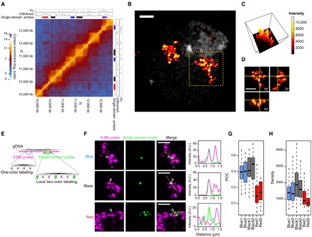
(A) S2R+ Hi-C map of the labeled 3-Mb region with chromatin immunoprecipitation (ChIP) tracks of Pc and H3K4me3. Colored bars denote the positions of probes designed to label specific epigenetic domains (Blue, Black, and Red). (B) 3D-SIM image of an S2R+ nucleus labeled with the 3-Mb probe (DAPI in gray). (C) Intensity distribution (maximum projection) of the 3-Mb probe in (B). (D) Orthogonal views of the 3-Mb probe labeling in (B). (E) Schematic representation of the dual FISH Oligopaint labeling strategy. gDNA, genomic DNA. (F) Examples of dual FISH labeling (maximum projections) with the 3-Mb probe and a single epigenetic domain (Blue1, Black2, or Red1, indicated with arrowheads). Right: Intensity distributions of the two probes along the yellow line. A.U., arbitrary units. (G) Pearson’s correlation coefficient (PCC) between the 3-Mb and the single-domain probe signals. Twenty nuclei were analyzed per conditions, and PCC distributions from all repressed domains were significantly different from those of active domains (at least P < 0.01) using Kruskal-Wallis and Dunn’s multiple comparisons tests. (H) Oligopaint density (probe genomic size over 3D-segmented volume) of the single-domain probes. At least 57 nuclei were analyzed per condition, and density distributions from all repressed domains were significantly different from those of active domains (at least P < 0.05) using Kruskal-Wallis and Dunn’s multiple comparisons tests. Scale bars, 1 μm.

TAD-based 3D nanocompartments undergo dynamic cis and trans contact events

These data suggest that Hi-C patterns resulting from cell population average studies might reflect the partitioning of chromatin into physical entities in Drosophila chromosomes, organized in the cell nucleus as discrete compact chromatin nanocompartments (repressive TADs), interspersed by more open regions (active domains). To test this hypothesis, we asked whether the number of observed nanocompartments corresponds to the number of repressed TADs. Of importance for this study, most nuclei in Dipteran species like Drosophila have paired homologous chromosomes in interphase. Chromosome pairing has been shown to be important for appropriate gene regulation (27), but the ultrastructure of paired homologous loci is still unknown. Whereas conventional WF microscopy often showed single unresolved foci for probes covering a single TAD, 3D-SIM resolved distinct nanocompartments (fig. S3, A and B). To address whether they correspond to the homologous TADs, we compared the numbers of foci observed in tetraploid S2R+ cells versus diploid embryonic (12 to 16 hours) cells, which have conserved TAD structures in Hi-C maps (fig. S4). In addition to single TADs and the 3-Mb probe that contains 12 repressed TADs, we designed additional Oligopaint probes: R2 (195 kb), R3 (805 kb), and R4 (495 kb), covering two, three, and four repressed TADs, respectively (fig. S4). We systematically observed an approximately twofold difference between the number of nanocompartments detected in tetraploid versus diploid cells, consistent with the predominant formation of juxtaposed yet spatially distinct TADs for each homolog in both cell types (Fig. 2, A and B). The distributions of the number of nanocompartments observed per cell indicated some degree of heterogeneity at the single-cell level. We could observe that homologous TADs can generate well-separated structures but also merge in a subset of the cells (fig. S3, C and D). Thus, chromatin fibers from paired homologous chromosomes do not appear to constantly intermingle, and instead, they form individual homologous TADs that engage in dynamic trans contact events. Some cells displayed more nanocompartments than would be expected based on the number of TADs multiplied by the ploidy (Fig. 2B). This observation was particularly evident for S2R+ cells, which have a sizeable proportion of G₂ cells, compared to embryonic cells, which are highly enriched in the G₀/G₁ phase of the cell cycle (28). To test whether these distributions could reflect differences in cell cycle stage and the fact that G₂ cells have replicated their DNA, we separated S2R+ cells into G₁ and G₂ populations based on DAPI signal (see Materials and Methods and fig. S5) (29). We could count more nanocompartments on average after replication, suggesting that, similar to chromosome homologs, sister chromatids behave largely as non-intermingled series of TADs (Fig. 2, C and D), consistent with the TADs observed by Hi-C in Drosophila polytene chromosomes (30). Moreover, there are very strong correlations between the mean number of nanocompartments observed and the number of TADs expected in both G₁ S2R+ cells and G₀/G₁ embryonic cells (Fig. 2E). To assess chromatin folding into TADs independently of pairing events, we also analyzed cells showing distinctly unpaired unique chromosomes, labeled with the 3-Mb probe (fig. S3E). We noticed heterogeneity in the higher-order arrangement of these TADs, ranging from a compact conformation to rarer unfolded chromosomes (Fig. 2, F and G). In this latter state, we were able to measure an average (±SD) nanocompartment diameter of 175 ± 27 nm (fig. S3, F and G). Again, the range of the number of nanocompartments detected in individual chromosomes fitted with the 12 repressed TADs predicted by Hi-C (Fig. 2H), although several cells showed a number of objects different from the expected number, suggesting that individual nanocompartments may contain multiple or split TADs. We thus conclude that the number of nanocompartments corresponds well with the number of repressed TADs, with a degree of cell-to-cell stochasticity due to the dynamics of intra- and inter-TAD contact events.

Fig. 2. Repressed TADs form 3D chromosomal units with dynamic contact events.

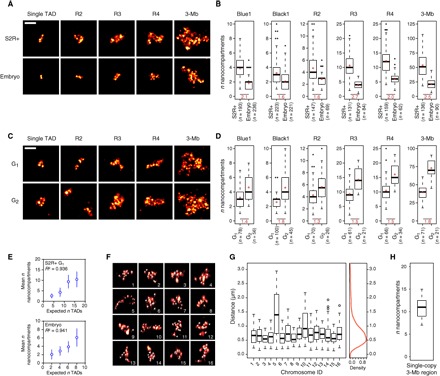
(A) Examples of chromatin labeling (single Black1 TAD, R2, R3, R4, and 3-Mb probe, maximum projections) in (top) tetraploid S2R+ and (bottom) diploid embryonic cells. (B) Number of nanocompartments counted per nucleus in S2R+ and embryonic cells for the different labeling (P < 0.0001 in all conditions with two-tailed Mann-Whitney test). Bottom: Ratio of the means (indicated with red circles) between the two conditions. n indicates the number of nuclei analyzed. (C) Examples of chromatin labeling (single Blue1 TAD, R2, R3, R4, and 3-Mb probe, maximum projections) in tetraploid S2R+ cells in (top) G₁ and (bottom) G₂ phases of the cell cycle. (D) Number of nanocompartments counted per nucleus in S2R+ cells in G₁ and G₂ phases for the different labeling (P < 0.0001 in all conditions with two-tailed Mann-Whitney test, except for R2, P < 0.01). Bottom: Ratio of the means (indicated with red circles) between the two conditions. n indicates the number of nuclei analyzed. (E) Mean (±SD) number of nanocompartments counted per S2R+ cells in G₁ phase (top) or in embryonic cells (bottom) as a function of the number of TADs for Black1, R2, R3, and R4 labeling. R² values of linear regressions are indicated. (F) 3D view of single chromosome copies labeled with the 3-Mb probe. Nanocompartment positions are represented with 150-nm-diameter beads. (G) Pairwise distances between all nanocompartments identified in the individual chromosomes shown in (F) (one boxplot corresponds to one chromosome). Right: Averaged distance distribution from all the single chromosomes. (H) Number of nanocompartments counted for single chromosomes (n = 19). Scale bars, 1 μm.

Repressed TADs form physical and structural chromosomal units

To rigorously quantify the single-cell variability of TAD behavior, we turned our analysis to TADs in a haploid context. We focused on a 400-kb region containing two distinct repressed TADs (Black) separated by an active region on the X chromosome of male embryos (Fig. 3A). We first used three-color FISH to measure intra-TAD (probes 2-1) versus inter-TAD (probes 2-3) 3D distances, with probes 1 and 3 being at the exact same genomic distance from probe 2. Our analysis revealed that intra-TAD distances are considerably shorter than inter-TAD distances (Fig. 3B). Moreover, inter-TAD distance distributions (1-3 and 2-3) were very similar, consistent with TAD structure strongly modulating the interdependence between physical and genomic distances. In support of this, analysis of FISH signal triplets showed that 75% of the 2-1 intra-TAD distances were shorter than the paired 2-3 inter-TAD distances (78% when considering the paired 1-3 inter-TAD distances; Fig. 3C). Previous studies compared 3D spatial distances between FISH probes corresponding to distinct regions and Hi-C interaction profiles (17, 20, 31), but the relationship between distance distribution and local chromatin conformation still remains unclear. We thus designed Oligopaint probes covering each single TADs independently (TAD 1 and TAD 2 probes), a probe of the same genomic size as TAD 1 but shifted to span the boundary (spanning probe), and a probe covering the entire region (full probe; Fig. 3A). We performed 3D-SIM imaging (Fig. 3D and fig. S6A) and observed that TAD 1 and TAD 2 displayed only one nanocompartment in the majority of cells, whereas most spanning and full probes were split into two or more nanocompartments, providing strong evidence for the physical compartmentalization of chromatin into TADs (Fig. 3E and fig. S6B). We then visualized TAD 1 and spanning probes using direct stochastic optical reconstruction microscopy (dSTORM) (32, 33). Image analysis using this independent method confirmed that TAD 1 appeared as a single nanocompartment in the majority of cells, unlike most spanning probes (fig. S7), despite their same genomic size. Analysis of the sphericity of the 3D-segmented probes also revealed that single TADs have highly globular structures compared to the spanning and full regions (fig. S6C). Globular single TADs have a similar diameter range as the nanocompartments described above within larger chromosomal regions [mean ± SD, 192 ± 35 nm (TAD 1) and 182 ± 23 nm (TAD 2); fig. S6D], consistent with nanocompartments corresponding to TADs. We could occasionally resolve numerous substructures in TADs of haploid cells (Fig. 3, D and E, and fig. S6, A and B), arguing for a dynamic behavior of TAD conformations in a subset of the cells. Finally, to further explore whether TADs represent distinct physical units, we labeled the two repressed TADs in different colors. Inter-TAD contacts were not observed in 68% of the nuclei, and less than 10% of volume overlap was detected in 84% of cases (Fig. 3F). This result strongly suggests that inter-TAD contacts reflect restricted chromatin interactions, rather than TAD merging. We thus conclude that, despite variable intra- and inter-TAD contacts in each cell, the physical TAD-based compartmentalization of the chromatin fiber is a general feature of chromosomal domains.

Fig. 3. Single-cell analysis of haploid chromosome reveals consistent TAD-based chromatin compartmentalization.

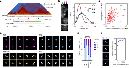
(A) Sixteen- to 18-hour male embryo Hi-C map with H3K4me3 ChIP-seq profile (14- to 16-hour embryos) and FISH probe positions. (B) Representative examples of triple FISH-labeled nuclei (confocal microscopy, z slices) with probes 1 (green), 2 (red), and 3 (blue) and 3D distance distributions (from 115 nuclei) between the probes. (C) Scatter plot of paired distances between probes 2 and 1 (x axis) and probes 2 and 3 (y axis). The proportions of intra-TAD (2-1) distances shorter or larger than inter-TAD (2-3) distances are indicated (75 and 25%, respectively). (D) Representative examples of 3D-SIM images (maximum projections) of TAD 1, TAD 2, spanning, and full probes. (E) Number of FISH local maxima detected per nucleus with the different probes (at least 102 nuclei were analyzed per condition). (F) Representative examples of 3D-SIM images (maximum projections) of TAD 1 and TAD 2 double FISH experiments and quantification of the overlap fraction between TAD 1 and TAD 2 probes (38 nuclei were analyzed). Statistics were performed with Kruskal-Wallis and Dunn’s multiple comparisons tests. ***P < 0.0001. Scale bars, 1 μm.

Polymer modeling recapitulates the physical partitioning of chromosomes into TADs

We then tested whether TAD compartmentalization can be predicted by using a self-avoiding and self-interacting polymer model (34, 35). First, we built a model of the same region described above, with monomers of 2 kb in which model parameters were fitted to reproduce the Hi-C data available for the same region (see Materials and Methods, Fig. 4A, and fig. S8, A and B). From the inferred ensemble of configurations, we computed distances for monomers corresponding to probes 1, 2, and 3 used in FISH (see Materials and Methods and Fig. 3A), and the comparison between model and FISH data shows a very good fit of the distance distributions (fig. S8C). The frequency for inter-TAD probe (2-3) distances smaller or equal to intra-TAD probe (2-1) distances is 15 ± 2%, in good agreement with experimental data (Fig. 4B and fig. S8D). To assess how changes in distances influence TAD structure (fig. S8E), we then used the inferred model to measure the overlap fraction (fig. S8F) for all simulated configurations or only for configurations where the inter-TAD probe (2-3) distance was smaller than the intra-TAD probe (2-1) distance. The configurations from the inferred model displayed weak overlap fraction between the TADs (≤10% overlap in 94% of the inferred configurations; Fig. 4C). Strikingly, the small overlap of TADs largely persists for configurations where the intra-TAD distance is higher than the inter-TAD distance (≤10% overlap in 85% of the inferred configurations; Fig. 4C). Therefore, polymer modeling using parameters that fit Hi-C maps supports the frequent folding of the two TADs into well-separated nanocompartments. The fraction of intra-TAD distances larger than the inter-TADs counterparts is thus explained by the dynamic relative positioning of the two TADs, rather than by TAD intermingling (Fig. 4D and fig. S8E). Overall, our microscopy and simulation results are consistent with TADs representing physical units of chromatin folding.

Fig. 4. Integrative view of chromosome conformation with polymer modeling.

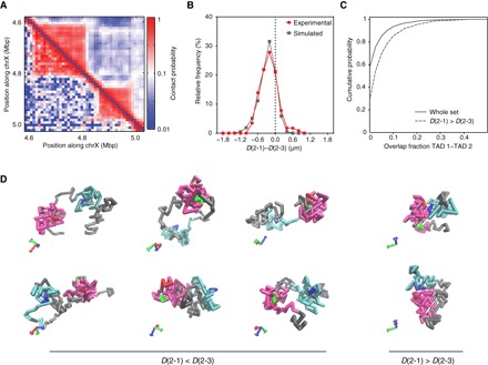
(A) Inferred (top) and experimental (bottom) contact probability maps. (B) Distributions of the differences between the paired distances (D) (2-1) and (2-3) from FISH experiments (red) and inferred model (gray). Values on the left of the dashed line indicate shorter intra-TAD than inter-TAD distances. (C) Cumulative distribution of the overlap fraction between TAD 1 and TAD 2 obtained from simulated conformations (full line) and from conformations when the inter-TAD distance (2-3) is smaller than the intra-TAD (2-1) distance (dashed line). (D) Representative examples of configurations of the inferred model, with the inter-TAD distance (2-3) larger (left) or smaller (right) than the intra-TAD (2-1) distance. Probe 1, 2, and 3 positions are represented with monomers in green, red, and blue, respectively; TAD 1 and TAD 2 are represented with magenta and cyan monomers, respectively.

Large-scale chromatin folding reflects highly heterogeneous yet specific, long-range interdomain contacts

Finally, we asked whether large-scale active and repressed compartments (2, 11) also represent physical entities or rather reflect statistical contact preference between highly heterogeneous chromosome configurations. We labeled chromatin domains of different epigenetic states and studied their relative 3D spatial organization (Fig. 5, A and B). This analysis revealed the presence of discrete interdomain contacts, with preference for contacts among TADs of the same epigenetic type (Fig. 5, C and D). These inter-TAD contacts are regulated, as the disruption of the polyhomeotic (ph) PcG gene specifically affects Pc inter-TAD contacts (36) without affecting contacts between other domains (Fig. 5, E to G). However, they are rare and the overall FISH configurations generated by the probe sets are highly heterogeneous (Fig. 5C). These results, consistent with previous reports (17, 18), suggest that active and repressive compartments reflect stochastic inter-TAD contacts with statistical preference for TADs of the same kind. These findings thus identify a difference between the nature of compartments defined from Hi-C, which is statistical, and that of repressive TADs, which are physical entities.

Fig. 5. Large-scale chromatin folding reflects heterogeneous, discrete, and specific interdomain contacts.

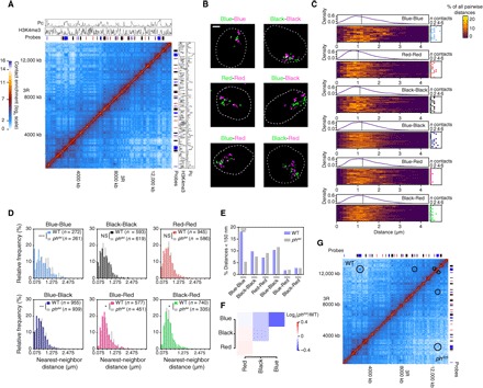
(A) Sixteen- to 18-hour embryo Hi-C map of a 14-Mb region, along with ChIP-seq profiles of Pc and H3K4me3 (14- to 16-hour embryos). We designed a set of epigenetic state-specific probes (Blue, Black, and Red domains, indicated with colored bars) to perform two-color labeling of domains of the same type that were consecutive along the linear scale of the chromosome (that is, Blue-Blue, Black-Black, and Red-Red) or for different combinations of chromatin type (that is, Blue-Black, Blue-Red, and Black-Red). (B) 3D-SIM images from different two-color FISH labeling combinations in embryonic cells (maximum projections). Scale bar, 1 μm. (C) Distribution of all the pairwise distances between all differentially labeled domains in the different FISH combinations. Each line of the heat maps represents distance distribution within single-cell (color-coded in the percentage of all the distances within the cell). On top of each heat map, the distribution of the distances for the whole cell population is plotted, and dashed line indicates median. On the right of each heat map, the number of distances is <150 nm per cell (n contacts). Twenty nuclei (>1800 distances in total) were analyzed per condition. The broad distributions in all FISH combinations indicate a limited extensive clustering of the domains of the same epigenetic status. (D) Nearest-neighbor distance distributions for each labeling combination in wild-type (WT) and ph^del 12- to 16-hour embryos. The x axis is split into 150-nm bins. n indicates the number of distances (measured in at least 30 nuclei) for each condition. Statistics were performed using Kolmogorov-Smirnov tests; ***P < 0.001, **P < 0.01, *P < 0.05. The depletion of very short range distances in Blue-Red and Black-Red distributions suggests that active chromatin is spatially segregated from inactive chromatin at the nanoscale. NS, not significant. (E) Percentages of nearest-neighbor distances <150 nm in WT embryos versus ph⁵⁰⁵ embryos, showing the specific loss of contacts between Blue domains. Statistics were performed using two-tailed Fisher’s exact tests, ***P < 0.0001. (F) Genome-wide differential Hi-C contact scores (log₂ ph⁵⁰⁵/WT normalized scores) between the chromatin domains in WT male versus ph⁵⁰⁵ male embryos show the specific loss of contacts between Blue domains. (G) Side-by-side Hi-C map of WT male (top) and ph⁵⁰⁵ male embryos (bottom) showing specific loss of contacts between Blue TADs in ph⁵⁰⁵ (indicated with circles). The contact enrichment color scale is the same as in (A).

DISCUSSION

This study demonstrates the partitioning of the chromatin fiber into discrete nanocompartments that correspond to repressed TADs intercalated with active chromatin domains. If individual TAD folding is dynamic and variable, then the meshwork of intra-TAD contacts is sufficient to hold them together to form nanocompartments. We thus propose that the high frequency and cooperativity, rather than the stability and the persistence, of intra-TAD interactions give rise to identifiable structures in single cells. Furthermore, the weak propensity of active chromatin, highly enriched in acetylated histones, to interact with inactive chromatin (7, 8) may be sufficient to shape a chromatin pattern made of a succession of segregated TAD-based discrete domains. These conclusions thus reconcile previous observations using microscopy and Hi-C (5, 6, 14, 17, 31, 34). Our data are consistent with TAD-based nanocompartments persisting through the interphase cell cycle, providing a role for TADs in the spatial segregation of autonomously regulated genomic regions. This chromosome organization is thus maintained in G₂ cells and may be the basis of chromosome pairing in interphase insect cells. Finally, the fact that TAD identity and architecture depend on cell fate regulation (15, 37) calls for further analysis in different cell types and species to generalize these findings and understand the mechanistic basis of the relation between 3D chromosome organization and chromatin contact patterns.

MATERIALS AND METHODS

Experimental design

Probe design and synthesis

Oligopaint libraries were constructed following the procedures described by Beliveau et al. (24) [see the Oligopaints website (http://genetics.med.harvard.edu/oligopaints) for further details]. The 3-Mb (chr2L: 9935314-12973080) library, synthesized at the Wyss Institute (Harvard University, Boston, MA), was a gift from the laboratory of C.-T. Wu (Harvard Medical School, Boston, MA). All other libraries were ordered from CustomArray in the 12K Oligo pool format. Coordinates, size, number, and density of probes for the libraries are given in table S1.

All libraries consisted of 42-mer genomic sequences discovered by OligoArray 2.1 run in the laboratory of C.-T. Wu with the following settings: -n 30 -l 42 -L 42 -D 1000 -t 80 -T 99 -s 70 -x 70 -p 35 -P 80 -m ‘GGGG;CCCC;TTTTT;AAAAA’ -g 44. Each library contains a universal primer pair followed by a specific primer pair hooked to the 42-mer genomic sequences (126-mers in total). Single TAD probe libraries allowing dual labeling (named “1:3”) contained one oligonucleotide of three potential genomic targets.

The 3-Mb Oligopaint probe was produced by emulsion polymerase chain reaction (PCR) amplification using universal primers followed by a “one-step PCR” and the lambda exonuclease procedure (24). In this case, each oligonucleotide contained a single fluorochrome. All other Oligopaint libraries were produced by emulsion PCR amplification from oligonucleotide pools followed by a “two-step PCR” procedure and the lambda exonuclease method (24). The two-step PCR leads to secondary oligonucleotide binding sites for signal amplification with a secondary oligonucleotide (Sec1 or Sec6) containing two additional fluorochromes. In this case, each oligonucleotide carried three fluorochromes in total. All oligonucleotides used for Oligopaint production were purchased from Integrated DNA Technologies. All oligonucleotide sequences (5′→3′) are listed below:

Emulsion PCR with universal primers

BB297-FWD: GACTGGTACTCGCGTGACTTG

BB299-REV: GTAGGGACACCTCTGGACTGG

3-Mb probe one-step PCR

BB291-FWD: /5Phos/CAGGTCGAGCCCTGTAGTACG

BB292-REV-ATTO565: /5ATTO565N/CTAGGAGACAGCCTCGGACAC

Two-step PCR

PCR1 with FWD 5′ phosphorylation and REV 53-mers:

A BB82-FWD: /5Phos/GTATCGTGCAAGGGTGAATGC

SecX-BB278-REV: /SecX/GAGCAGTCACAGTCCAGAAGG

B BB81-FWD: /5Phos/ATCCTAGCCCATACGGCAATG

SecX-BB281-REV: /SecX/GGACATGGGTCAGGTAGGTTG

C BB287-FWD: /5Phos/CGCTCGGTCTCCGTTCGTCTC

SecX-BB288-REV: /SecX/GGGCTAGGTACAGGGTTCAGC

D BB293-FWD: /5Phos/CCGAGTCTAGCGTCTCCTCTG

SecX-BB294-REV: /SecX/AACAGAGCCAGCCTCTACCTG

E BB298-FWD: /5Phos/CGTCAGTACAGGGTGTGATGC

SecX-BB187-REV: /SecX/TTGATCTTGACCCATCGAAGC

Binding sequence Sec1: CACCGACGTCGCATAGAACGGAAGAGCGTGTG

Binding sequence Sec6: CACACGCTCTCCGTCTTGGCCGTGGTCGATCA

PCR2 with labeled “back primer”

BB506-Alexa488: /5Alex488N/CACCGACGTCGCATAGAACGG

BB511-Cy3: /5Cy3/CACACGCTCTCCGTCTTGGC

BB511-ATTO565: /5ATTO565N/CACACGCTCTCCGTCTTGGC

Secondary oligos

Sec1-Alexa488-X2: /5Alex488N/CACACGCTCTTCCGTTCTATGCGACGTCGGTGagatgttt/3AlexF488N/

Sec6-Cy3-X2: /5Cy3/TGATCGACCACGGCCAAGACGGAGAGCGTGTGagatgttt/3Cy3Sp/

Sec6-ATTO565-X2: /5ATTO565N/TGATCGACCACGGCCAAGACGGAGAGCGTGTGagatgttt/3ATTO565N/

Sec6-Alexa488-X2: /5Alex488N/TGATCGACCACGGCCAAGACGGAGAGCGTGTGagatgttt/3AlexF488N/

In Fig. 5, for the labeling of domains of the same chromatin type (that is, Blue-Blue, Black-Black, and Red-Red), domains that were consecutive along the chromosome were alternatively labeled, that is, one in A488 followed by one in Cy3 or ATTO565, etc. For this purpose, the oligopools corresponding to nonconsecutive domains of the same chromatin type were on the same array, which allows their amplification as one library using the same primer set. For the labeling of domains of different chromatin type (that is, Blue-Black, Blue-Red, and Black-Red), all domains of the same chromatin type were labeled using one color.

Small probes 1, 2, and 3 used for triple FISH experiments (Fig. 3) were generated using four consecutive PCR fragments of 1.1 to 1.6 kb from Drosophila genomic DNA, each covering approximately 8 kb. The list below shows the amplicon size (bp) and the corresponding primers for each probe fragment.

Probe 1
Fragment 1	1299	1_FWD	AGGTGGAGTTGTGTATGCGA
		1_REV	GAGTGAAAAGGCGTTGGTGT
Fragment 2	1568	2_FWD	TCCACTTTCGCCTGATGTCT
		2_REV	GAGGTGTTTGTGCCAGGAAG
Fragment 3	1084	3_FWD	TTTCTTACCCCATCCACCCC
		3_REV	TATAAGCCCGGCCAAGTTGA
Fragment 4	1443	4_FWD	GAGCTGGGACGTAACCTCTT
		4_REV	ATGTTCACGCTTCTCCTCGA

Probe 2
Fragment 1	1446	1_FWD	CAGCGTGAGTGTCAAGTGAG
		1_REV	GCTGATGTTTTGGCTTCCGA
Fragment 2	1568	2_FWD	TGAAATACGACGAACCGCAG
		2_REV	TGTTTCGACTGTAAAGCCGC
Fragment 3	1310	3_FWD	CTGGGCGACAAGAACAACAA
		3_REV	AAGAAAATTGCCAGCCCCAG
Fragment 4	1305	4_FWD	TAACCAATTGCCGCGTTGAA
		4_REV	AAATCGGTGGGTGATGAGGT

Probe 3
Fragment 1	1421	1_FWD	CCACAAGAAAAGCACCCACA
		1_REV	TCTCGCTCTGTTCAAGGTGT
Fragment 2	1243	2_FWD	CCTCAGCAGCTTTTCGGATC
		2_REV	GCCCCGGATTGTTGATTCTC
Fragment 3	1481	3_FWD	ACCTCTACGCTCCAGATTCG
		3_REV	AGTGCTTATCAACGACCCCA
Fragment 4	1292	4_FWD	GCTCGCTCATTTGACCCAAT
		4_REV	CTTTCCGCTCATCTTGGGTG

Probes were labeled using the FISH Tag DNA Kit (Invitrogen Life Technologies) with Alexa Fluor 488, 555, and 647 dyes. All probe coordinates refer to Dm3/FlyBase R5 reference genome.

Three-dimensional FISH

3D-FISH was adapted from Bantignies and Cavalli (38). For optimal imaging, we used coverslips of 0.170 ± 0.005 mm (Zeiss). Coverslips were rinsed in 96% ethanol before incubation for 5 min in 1:10 poly-l-lysine (P8920, Sigma-Aldrich) diluted in water (final concentration at 0.01%, w/v). Briefly, cells in suspension (about 2 × 10⁶ cells/ml) were deposited on a coverslip for 1-hour sedimentation in a humid chamber, or four to five dechorionated and selected embryos were squeezed directly on a coverslip with a Dumont #55 tweezer. Samples were fixed with phosphate-buffered saline (PBS)/4% paraformaldehyde (PFA), washed in PBS, permeabilized with PBS/0.5% Triton X-100 for 10 min, washed in PBS, and incubated for 30 min in PBS/20% glycerol. After PBS washes, cells were incubated with 0.1 M HCl for 10 min, washed in 2× SSCT (2× SSC/0.1% Tween 20), and incubated for 30 min in 50% formamide, 2× SSCT. Probe mixture contains 20 pmol of each probe with 20 pmol of their complementary secondary oligonucleotide (except for the 3-Mb region, used without secondary oligo), 0.8 μl of ribonuclease A (10 mg/ml), and FISH hybridization buffer [FHB; 50% formamide, 10% dextran sulfate, 2× SSC, and salmon sperm DNA (0.5 mg/ml)], in a total mixture volume of approximately 20 to 25 μl, keeping at least a 3:4 ratio of FHB/total volume. Probe mixture was added to the coverslip before sealing on a glass slide with rubber cement (Fixogum, Marabu). Cell DNA was denatured at 78°C for 3 min, and hybridization was performed at 37°C overnight in a humid dark chamber. Cells were then washed 3 × 5 min at 37°C in 2× SSC, 3 × 5 min at 45°C in 0.1× SSC, and 2 × 5 min in PBS before DNA counterstaining with DAPI (final concentration at 0.3 mg/ml in PBS). After final washing in PBS, coverslips were mounted on slides with Vectashield (CliniSciences) and sealed with nail polish.

Immunostaining

Cells in suspension (about 2 × 10⁶ cells/ml) were deposited on coverslips for 1-hour sedimentation in a humid chamber. Cells were fixed in PBS/4% PFA, washed in PBS, treated with PBS/0.1% Triton X-100 for 15 min, and washed in PBS/0.02% Tween 20 (PBT) before blocking in PBT/2% bovine serum albumin (BSA) (A7906, Sigma-Aldrich) for 30 min. Cells were then incubated with cyclin B (CycB) antibody (Developmental Studies Hybridoma Bank, product F2F4), diluted in PBT/2% BSA (1:500 dilution) overnight at 4°C in a humid chamber. Cells were then washed with PBT, incubated with secondary antibody (1:200 dilution; A-31570, Life Technologies) for 1 hour at room temperature, washed with PBT, and incubated in PBS and DAPI (final concentration at 0.5 mg/ml in PBS). Cells were then washed with PBS, and coverslips were mounted on slides with Vectashield (CliniSciences).

Image acquisition

3D-SIM super-resolution imaging was performed with a DeltaVision OMX V3/V4 microscope (GE Healthcare) equipped with a ×100/1.4 numerical aperture (NA) Plan Super Apochromat oil immersion objective (Olympus). Electron-multiplying charge-coupled device (EMCCD) (Evolve 512B, Photometrics) cameras for a pixel size of 79 nm at the sample were used. Diode lasers at 405, 488, and 561 nm and the standard corresponding emission filters were used. Z-stacks were acquired with five phases and three angles per image plane, with a z-step of 125 nm. Raw images were reconstructed using SoftWorx (version 6.5, GE Healthcare), using channel-specific optical transfer functions (pixel size of reconstructed images, 39.5 nm). TetraSpeck beads (200 nm) (T7280, Thermo Fisher Scientific) were used to calibrate alignment parameters between the different channels. Quality of reconstructed images was assessed using ImageJ and the SIMcheck plugin (39), and examples of quality controls are shown in fig. S9. Conventional WF images were generated from raw images using SoftWorx by averaging the different angles and phases for each plane. Automatic “Threshold and 16-bit Conversion” (SIMcheck plugin) was applied to the reconstructed images shown.

Confocal microscopy images were acquired with a Leica SP8 microscope (Leica Microsystems) equipped with a ×63/1.4 NA Plan-Apochromat oil immersion objective and photomultiplier tube and hybrid detectors for a pixel size of 59 nm (z-step, 300 nm).

dSTORM super-resolution imaging was carried out with a custom-made inverted microscope using an oil immersion objective (Plan-Apochromat, 100×, 1.4 NA oil DIC, Zeiss) mounted on a z-axis piezoelectric stage (P-721.CDQ, PICOF, PI). A 1.5× telescope was used to obtain a final imaging magnification of 150-fold corresponding to a pixel size of 105 nm. Two lasers were used for excitation/photoactivation: 642 nm (MPB Communications Inc.) and 405 nm (OBIS, LX 405-50, Coherent Inc.). Laser lines were expanded and coupled into a single beam using a dichroic mirror (427-nm LaserMUX, Semrock). An acousto-optic tunable filter (AOTFnc-400.650-TN, AA Opto-Electronics) was used to modulate laser intensity. Light was circularly polarized using an achromatic quarter wave plate. Two achromatic lenses were used to expand the excitation laser and an additional dichroic mirror (zt405/488/561/638rpc, Chroma Technology) to direct it toward the back focal plane of the objective. Fluorescence light was spectrally filtered with emission filters (ET700/75m, Chroma Technology) and imaged on an EMCCD camera (iXon X3 DU-897, Andor Technology). The microscope was equipped with a motorized stage (MS-2000, ASI) to translate the sample perpendicularly to the optical axis. To ensure the stability of the focus during the acquisition, a homemade autofocus system was built. A 785-nm laser beam (OBIS, LX 785-50, Coherent Inc.) was expanded twice and directed toward the objective lens by a dichroic mirror (z1064rdc-sp, Chroma Technology). The reflected infrared beam was redirected following the same path than the incident beam and guided to a CCD detector (Pixelfly, Cooke) by a polarized beam splitter cube. Camera, lasers, and filter wheel were controlled with software written in LabVIEW (40).

For image acquisition, an average of 15,000 frames was recorded at a rate of 10 ms per frame. To induce photoswitching, samples were imaged in a freshly prepared Smart Kit buffer (Abbelight). Continuous excitation and activation was used with output laser powers of 600 mW at 642 nm (for AF647 excitation) and 0 to 2.5 mW at 405 nm (for activation). The intensity of activation was progressively increased throughout the acquisition to ensure a constant amount of simultaneously emitting fluorophores within the labeled structures. These excitation powers were optimized to ensure single-molecule detection. Imaging data are available upon request.

Image analysis

3D image analysis was performed using Imaris software and its XT module. For all images analyzed in 3D, a background subtraction filter was applied. For fluorescence intensity correlation, the regions of interest were first segmented in 3D (the 3-Mb probe for fig. S1E or the single-domain probes for fig. S2B and Fig. 1G). PCCs were then calculated in single cell using the voxels within the regions of interest. To measure the probe density of the single domains (Fig. 1H), we divided the genomic size of the labeled regions by the volume occupied by the 3D-segmented probes (probes with full Oligopaint coverage) in each single nucleus analyzed. To count the number of nanocompartments in the different FISH experiments (and to identify the 3-Mb maxima in fig. S1F), we used the point-like structure function (spots) of Imaris. Examples of nanocompartment identification with this method are shown in Fig. 2F. Distances between nanocompartments were calculated between the centered voxels of the spots identified. The sizes of nanocompartments (figs. S3, F and G, and S6D) were determined using full width at half maximum of Gaussian curves fitted to the intensity profiles obtained along lines passing through single nanocompartments in z-stacked (maximum projections) images [processed with Threshold and 16-bit Conversion from SIMcheck (39)]. To investigate contact frequency and overlap between TAD 1 and TAD 2 (Fig. 3F), we segmented the probes in 3D and calculated the Jaccard index by dividing the volume of the colocalized voxels (intersection of the two probes) by the sum of the volumes of the segmented probes minus the colocalized volume (union of the volumes of the two probes). This Jaccard index was defined as the overlap fraction. The quantification of segmented objects (fig. S6B) was performed with ImageJ’s Otsu automatic thresholding of FISH signals (minimum size of 6 pixels²) in z-stacked (maximum projections) images (processed with Threshold and 16-bit Conversion from SIMcheck). Sphericity scores (fig. S6C) were calculated from probe 3D segmentation in individual nuclei. Specific epigenetic domains on the 3R chromosome (Fig. 5) were identified using the spot function of Imaris, and distances (all pairwise or nearest-neighbor distances) were measured in 3D from the centered voxels of the spots.

To measure the distances between small probes 1, 2, and 3 (Fig. 3, B and C), we applied a Gaussian filter (σ = 1 pixel) to the image before 3D segmentation of the spot signals and calculation of their center of mass. We then identified mutual nearest neighbors between the centers of mass of probes 2 and 1 and between the centers of mass of probes 2 and 3 and calculated combinatorial 3D distances for these triplets. To assess the experimental error, we used 200-nm TetraSpeck beads (T7280, Thermo Fisher Scientific) coupled with dyes of the same colors than the FISH probes, and we applied the same method for 3D distance measurements. We obtained from the beads a mean (±SD) of 164 ± 41 nm between red and green dyes (corresponding to probe 2 and 1 dyes, respectively), 107 ± 46 nm between red and far-red dyes (corresponding to probe 2 and 3 dyes, respectively), and 231 ± 67 nm between green and far-red dyes (corresponding to probe 1 and 3 dyes, respectively). This indicates that the shorter distance distribution between intra-TAD probes (2-1) compared to inter-TAD (2-3) is not due to technical bias.

For dSTORM image after processing and analysis, single-molecule localization was performed using the ImageJ ThunderSTORM plugin. Default values were used for the analysis (B-spline wavelet filter—order 3 and scale 2.0, approximate localization by eight-neighborhood local maximum, subpixel localization by point spread function (PSF)–integrated Gaussian with the weighted least squares fitting method with a 3-pixel fitting radius and 1.6-pixel initial sigma). Particle coordinates and statistical properties were exported, and further analysis was conducted using MATLAB (MathWorks). Clustering of localizations was performed using an algorithm that was previously described by Cattoni et al. (41). A particle density and area threshold was set to define and quantify the number of objects per imaged probe. Automatic detection and quantification were further verified by visual inspection and comparison of conventional fluorescence and super-resolution rendered images using variable intensity thresholds.

Determination of cell cycle stage

We used the method published by Roukos et al. (29) to determine cell cycle stages of S2R+ cells. This method is based on DAPI fluorescence intensity after microscopy image acquisition (fig. S5). Briefly, DAPI channels of images were separated and projected along the z axis using average intensity, and nuclei were identified with CellProfiler software (http://cellprofiler.org/). The DAPI-integrated intensity was calculated for each nucleus, and the distribution for the whole population was plotted. The nuclei were then classified as G₁ or G₂ according to their DAPI-integrated intensity profile relative to the profile obtained for the population (fig. S5). To classify nuclei positive for CycB (fig. S5C), the CycB signal was segmented using CellProfiler software, and overlapped nuclei were counted.

Hi-C library preparation and sequencing

For S2R+ cells, Hi-C and library preparation was performed using the in situ method as published by Rao et al. (11) with minor modifications. Two biological replicates were done using 5 × 10⁶ cells. Briefly, cells were digested overnight at 37°C using 500 U of Dpn II. After biotin filling, proximity ligation was carried out for 4 hours at 18°C with 2000 U of T4 DNA ligase, and after reverse cross-linking, DNA was purified with ethanol precipitation and sheared to 300- to 400-bp fragments using a Covaris S220 sonicator. Ligation fragments with biotin were pulled down using MyOne Streptavidin T1 beads (catalog no. 65602, Thermo Fisher Scientific), end-repaired, and adenylated as described. Fragments were then ligated with NEXTflex adaptors (catalog no. 514101, BioScientific) and amplified by PCR using the KAPA HiFi Library Amplification Kit (catalog no. KK2620, Kapa Biosystems) for eight cycles. DNA size selection (300 to 800 bp) was performed using AMPure XP beads (catalog no. A63881, Agencourt). Libraries were validated qualitatively and quantitatively with Fragment Analyzer and by qPCR (Roche LightCycler 480). They were sequenced with 2 × 50–bp paired-end runs on an Illumina HiSeq 2500.

For embryo Hi-C, embryos were collected in a saline buffer (0.03% Triton X-100, 0.4% NaCl) 16 to 18 hours after egg laying and then dechorionated for 5 min in fresh bleach. About 3000 GFP⁻ (selection of ph⁵⁰⁵ null mutant males; see the “Drosophila” section for description) and GFP⁺ (selection of WT males from the Y-GFP line) embryos each were sorted with a Union Biometrica COPAS large particle sorter (Union Biometrica Inc.) and then processed for Hi-C as in the study of Sexton et al. (6).

Hi-C analysis

Hi-C sequence mapping, read filtering, and normalization were performed as previously published (6). This provided statistics on the number of observed contacts for each pair of restriction fragments and the number of expected contacts from a low-level probabilistic model, which considers local GC content and the Dpn II restriction fragment length. Therefore, technically corrected matrices were generated by calculating ratios between the total observed reads and the expected reads based on the above model. We visualized contact maps as described by Sexton et al. (6). To maximize resolution, we used variable bin sizes from 5 to 160 kb, visualizing each point in the matrix using the ratio as computed for the minimal 2D bin with at least 30 observed contacts. S2R+ Hi-C map (Fig. 1A) was plotted based on merging two replicates for the 3-Mb region 2L:9935314..12973080 and aligned with the ChIP-sequencing (ChIP-seq) profile of Pc (S2 cells, GSM604723) and ChIP-chip of H3K4me3 (S2 cells, modENCODE305). Side-by-side Hi-C comparisons for R2 (2R:10534240..10729120), R3 (3R: 23547420..24352723), R4 (2R: 5203174..5698315), and the 3-Mb Oligopaint-labeled regions (fig. S4) show the contact map in S2R+ cells (merge of replicates) on the top left and embryos [16 to 18 hours, merge of two replicates published by Schuettengruber et al. (42)] on the bottom right, alongside with ChIP-seq of H3K4me3 (embryo 14 to 16 hours, modENCODE5096) and ChIP-chip of H3K4me3 (S2 cells, modENCODE305). The male embryo Hi-C map (Fig. 3A) is plotted based on merging two replicates for the region X:4502500..5061200 alongside with ChIP-seq of H3K4me3 (modENCODE5096). The embryo [16 to 18 hours, merge of two replicates published by Schuettengruber et al. (42)] Hi-C map (Fig. 5A) is plotted for the region 3R:500000..14000000 and aligned with ChIP-seq of Pc (modENCODE3957) and H3K4me3 (modENCODE5096). The side-by-side Hi-C comparison for the 3R:500000..14000000 region (Fig. 5G) shows the contact map in WT male embryos (merge of two replicates) on the top left and ph⁵⁰⁵ male embryos (merge of two replicates) on the bottom right. Data sets are available at GSE99107.

Cis-decay curve analysis

For each single domain (fig. S2E), the observed and expected interaction counts for different bins of genomic separation were computed (from 400 bp to the full TAD size and separated by at least two fragments). The expected scores were taken by computing over all possible pairwise fragment combinations. The observed scores were obtained by counting all interactions within Hi-C data, which correspond to a particular distance. The cis-decay curve was plotted as the observed/expected ratio (the probability of detecting a Hi-C interaction) over a particular genomic separation on a logarithmic scale.

Analysis of domain contacts between different chromatin colors

The boundaries of domains were demarcated using the topmost fifth percentile of 5 kb–smoothed inferred distance-scaling factors (6). Domains were merged when their length was smaller than 10 kb. Then, domains were colored as red, blue, and black according to k-means grouping results based on their average enrichments of H3K4me3, H3K27me3, HP1, and H1 marks (6). We generated a domain-level contact map by calculating ratios between observed contacts of associating fragments within each pair of domains and total expected contacts based on the distance-scaling model (factoring out the general tendency of adjacent domains to contact each other). Differential contacts between WT and ph null mutant male embryos are expressed as the log₂ ratio of the ph⁵⁰⁵ normalized contacts and the WT normalized contacts (Fig. 5F).

Polymer modeling of haploid chromatin regions

We modeled the genomic region of chromosome X located between 4.58 and 5.03 Mbp by a flexible self-avoiding polymer containing n = 225 monomers, each monomer, of size a, representing 2 kbp. The chain dynamics was mapped on a face-centered cubic lattice following the kinetic Monte-Carlo scheme described by Olarte-Plata et al. (35) driven by short-range contact interactions following the Hamiltonian

$$\mathit{H}={\displaystyle \sum _{\mathit{i}=1}^{\mathit{n}}}{\displaystyle \sum _{\mathit{j}=\mathit{i}+1}^{\mathit{n}}}{\mathit{U}}_{\mathit{i},\mathit{j}}{\mathrm{\delta }}_{\mathit{i},\mathit{j}}$$

where U_i,j is the energy of interaction between monomers i and j, and δ_i,j = 1 if the two monomers are nearest neighbor on the lattice, and δ_i,j = 0 otherwise.

Parameters {U_i,j} were inferred such that the predicted contact map at equilibrium is consistent with experiments. The corresponding target contact map (Fig. 4A, bottom) was derived from the experimental Hi-C map at 10-kbp resolution: Similar to previous work (43), we transformed the experimental normalized contact frequencies C_k,l into contact probabilities P_k,l (the observable that we can directly compare to simulations) using the following procedure: ${\mathit{P}}_{\mathit{k},\mathit{l}}= \text{min}\left(1\frac{{\mathit{C}}_{\mathit{k},\mathit{l}}}{{\overline{\mathit{C}}}_{\pm 1}}\right),$ where ${\overline{\mathit{C}}}_{\pm 1}$ is the median value of {C_k,k+1}. The underlying assumption is that in a polymer model, adjacent monomers are always in contact. Note that in our polymer model, a 10-kbp region (the experimental resolution we used to avoid too much sampling noise) is represented by five consecutive beads. Therefore, for a given simulated configuration, two 10-kbp regions will be predicted to be in contact if at least one 2-kbp monomer of the first region is closest than a cutoff distance R to a monomer of the second region. R corresponds to the maximal distance between two loci that is captured by Hi-C experiments as a contact. Using this definition, for a given set of parameters {U_i,j} and a given value of R, we estimated the corresponding contact probability map at 10-kbp resolution from the sampling of 10,000 configurations at equilibrium (examples of configurations are given in Fig. 4D). For a fixed R, the values of {U_i,j} were inferred by minimizing the χ² score

$${\mathrm{\chi }}^2={\displaystyle \sum _{\mathit{k},\mathit{l}}}\frac{{[{\mathit{P}}_{\mathit{k},\mathit{l}}(\text{sim})-{\mathit{P}}_{\mathit{k},\mathit{l}}(\text{exp})]}^2}{{\mathrm{\sigma }}_{\mathit{k}\mathit{l}}^2(\text{exp})}$$

where ${\mathrm{\sigma }}_{\mathit{k}\mathit{l}}^2(\text{exp})$ is the standard error of P_k,l(exp) estimated using experimental replicates. We followed the scheme developed by Giorgetti et al. (34) that makes use of Boltzmann reweighting to numerically speed up the inference. Using this technique, convergence to a local minimum of χ² is fast (fig. S8B). We repeated this operation several times by varying also the values of R and took the realization with the lowest local minimum (Fig. 4A and fig. S8B for R = 1.4a). The length unit in the simulation (a = 102 ± 4 nm) was then fixed by comparing the predicted distances between the three loci investigated by FISH to the corresponding experimental data accounting for a random experimental error of ~100 nm (fig. S8C; see the “Image analysis” section for the calculation of the experimental error).

For a given simulated configuration, the overlap fraction between TAD 1 and TAD 2 was computed by estimating the 3D convex envelope of each TAD using the MATLAB function convexhull and by computing the fraction of TAD 1 and TAD 2 monomers belonging to both envelopes (an illustration in 2D is given in fig. S8F). An overlap fraction of 0 (resp. 1) signifies that both TADs occupy separate (resp. common) volumes.

Cell culture

S2R+ cells (stock #150, Drosophila Genomics Resource Center) were grown at 25°C in Schneider’s S2 medium (S0146, Sigma-Aldrich) complemented with 10% fetal bovine serum (FBS) (10500064, Gibco) and 1% penicillin-streptomycin (15140122, Gibco).

For S2R+ Hi-C, cells were incubated with enhanced green fluorescent protein (EGFP) double-stranded RNA (dsRNA). For each well (six-well plate), 1 × 10⁶ cells in 1-ml serum-free medium were deposited with 17.5 μg of dsRNA and incubated for 30 min before addition of 2 ml of medium with 15% FBS. Cells were then grown for 5 days at 25°C before harvest. EGFP dsRNAs were obtained from plasmid PCR amplification (sequences given below), followed by in vitro transcription using the MEGAscript Kit (Ambion Inc.):

EGFP FWD-primer: 5′-T7-GACGTAAACGGCCACAAGTT-3′

EGFP REV-primer: 5′-T7-TGCTCAGGTAGTGGTTGTCG-3′

T7 sequence: 5′-TAATACGACTCACTATAGGG-3′

EGFP amplicon sequence: GACGTAAACGGCCACAAGTTCAGCGTGTCCGGCGAGGGCGAGGGCGATGCCACCTACGGCAAGCTGACCCTGAAGTTCATCTGCACCACCGGCAAGCTGCCCGTGCCCTGGCCCACCCTCGTGACCACCCTGACCTACGGCGTGCAGTGCTTCAGCCGCTACCCCGACCACATGAAGCAGCACGACTTCTTCAAGTCCGCCATGCCCGAAGGCTACGTCCAGGAGCGCACCATCTTCTTCAAGGACGACGGCAACTACAAGACCCGCGCCGAGGTGAAGTTCGAGGGCGACACCCTGGTGAACCGCATCGAGCTGAAGGGCATCGACTTCAAGGAGGACGGCAACATCCTGGGGCACAAGCTGGAGTACAACTACAACAGCCACAACGTCTATATCATGGCCGACAAGCAGAAGAACGGCATCAAGGTGAACTTCAAGATCCGCCACAACATCGAGGACGGCAGCGTGCAGCTCGCCGACCACTACCAGCAGAACACCCCCATCGGCGACGGCCCCGTGCTGCTGCCCGACAACCACTACCTGAGCA

Drosophila

For the FISH experiments, flies were raised in standard cornmeal yeast extract media at 21°C. Embryos were harvested on agar/vinegar plate at stages 15 to 16 after egg laying, equivalent to a development of 12 to 16 hours at 25°C. Embryos were manually dechorionated on a double-face adhesive tape and displayed on an agar/vinegar plate to avoid drying during manual selection under a GFP binocular. The Oregon-R w[1118] line was used as the WT control line. To analyze haploid regions on chromosome X in male embryos, a Y-GFP reporter line (Y-GFP line: y[1], w[67c23]; Dp(1;Y), y[+] P{ry+11} P{w[+mC]=ActGFP}JMR1) was used for the selection of WT GFP⁺ male embryos. This line was a gift of S. Hayashi and is described by Hayashi (44). The ph^del stock was balanced over the KrGFP-FM7c balancer (obtained from BL#5193 of the Bloomington Drosophila Stock Center) for the selection of hemizygous ph^del GFP⁻ null mutant male embryos. The ph^del stock was a gift from the laboratory of J. Wang.

For embryo Hi-C, flies were raised in standard cornmeal yeast extract media at 25°C. The ph⁵⁰⁵ stock was balanced over the KrGFP-FM7c balancer for the selection of hemizygous ph⁵⁰⁵ GFP⁻ null mutant male embryos. The Y-GFP line described above was used for the selection of WT GFP⁺ male embryos to be compared with the ph mutant male embryos.

Statistical analysis

Description of statistical analysis is included in the figure legends.

SUPPLEMENTARY MATERIALS

Supplementary material for this article is available at http://advances.sciencemag.org/cgi/content/full/4/2/eaar8082/DC1

fig. S1. Chromatin nanostructure visualization with 3D-SIM imaging.

fig. S2. Dual labeling Oligopaint FISH.

fig. S3. Resolution of homologous TADs with 3D-SIM.

fig. S4. Oligopaint probe–targeted regions in S2R+ cells and embryos.

fig. S5. Cell cycle staging of S2R+ cells.

fig. S6. Super-resolution imaging of haploid chromatin folding.

fig. S7. 2D dSTORM imaging of TAD 1 and spanning probes.

fig. S8. Modeling the X chromatin region.

fig. S9. Quality control of SI acquisitions.

table S1. Libraries for Oligopaint probes.

REFERENCES AND NOTES

- 1.Bonev B., Cavalli G., Organization and function of the 3D genome. Nat. Rev. Genet. 17, 661–678 (2016). [DOI] [PubMed] [Google Scholar]
- 2.Lieberman-Aiden E., van Berkum N. L., Williams L., Imakaev M., Ragoczy T., Telling A., Amit I., Lajoie B. R., Sabo P. J., Dorschner M. O., Sandstrom R., Bernstein B., Bender M. A., Groudine M., Gnirke A., Stamatoyannopoulos J., Mirny L. A., Lander E. S., Dekker J., Comprehensive mapping of long-range interactions reveals folding principles of the human genome. Science 326, 289–293 (2009). [DOI] [PMC free article] [PubMed] [Google Scholar]
- 3.Dixon J. R., Selvaraj S., Yue F., Kim A., Li Y., Shen Y., Hu M., Liu J. S., Ren B., Topological domains in mammalian genomes identified by analysis of chromatin interactions. Nature 485, 376–380 (2012). [DOI] [PMC free article] [PubMed] [Google Scholar]
- 4.Hou C., Li L., Qin Z. S., Corces V. G., Gene density, transcription, and insulators contribute to the partition of the Drosophila genome into physical domains. Mol. Cell 48, 471–484 (2012). [DOI] [PMC free article] [PubMed] [Google Scholar]
- 5.Nora E. P., Lajoie B. R., Schulz E. G., Giorgetti L., Okamoto I., Servant N., Piolot T., van Berkum N. L., Meisig J., Sedat J., Gribnau J., Barillot E., Blüthgen N., Dekker J., Heard E., Spatial partitioning of the regulatory landscape of the X-inactivation centre. Nature 485, 381–385 (2012). [DOI] [PMC free article] [PubMed] [Google Scholar]
- 6.Sexton T., Yaffe E., Kenigsberg E., Bantignies F., Leblanc B., Hoichman M., Parrinello H., Tanay A., Cavalli G., Three-dimensional folding and functional organization principles of the Drosophila genome. Cell 148, 458–472 (2012). [DOI] [PubMed] [Google Scholar]
- 7.Rowley M. J., Nichols M. H., Lyu X., Ando-Kuri M., Rivera I. S. M., Hermetz K., Wang P., Ruan Y., Corces V. G., Evolutionarily conserved principles predict 3D chromatin organization. Mol. Cell 67, 837–852.e7 (2017). [DOI] [PMC free article] [PubMed] [Google Scholar]
- 8.Ulianov S. V., Khrameeva E. E., Gavrilov A. A., Flyamer I. M., Kos P., Mikhaleva E. A., Penin A. A., Logacheva M. D., Imakaev M. V., Chertovich A., Gelfand M. S., Shevelyov Y. Y., Razin S. V., Active chromatin and transcription play a key role in chromosome partitioning into topologically associating domains. Genome Res. 26, 70–84 (2016). [DOI] [PMC free article] [PubMed] [Google Scholar]
- 9.Haarhuis J. H. I., van der Weide R. H., Blomen V. A., Yáñez-Cuna J. O., Amendola M., van Ruiten M. S., Krijger P. H. L., Teunissen H., Medema R. H., van Steensel B., Brummelkamp T. R., de Wit E., Rowland B. D., The cohesin release factor WAPL restricts chromatin loop extension. Cell 169, 693–707.e14 (2017). [DOI] [PMC free article] [PubMed] [Google Scholar]
- 10.Nora E. P., Goloborodko A., Valton A. L., Gibcus J. H., Uebersohn A., Abdennur N., Dekker J., Mirny L. A., Bruneau B. G., Targeted degradation of CTCF decouples local insulation of chromosome domains from genomic compartmentalization. Cell 169, 930–944.e22 (2017). [DOI] [PMC free article] [PubMed] [Google Scholar]
- 11.Rao S. S. P., Huntley M. H., Durand N. C., Stamenova E. K., Bochkov I. D., Robinson J. T., Sanborn A. L., Machol I., Omer A. D., Lander E. S., Aiden E. L., A 3D map of the human genome at kilobase resolution reveals principles of chromatin looping. Cell 159, 1665–1680 (2014). [DOI] [PMC free article] [PubMed] [Google Scholar]
- 12.Rao S. S. P., Huang S.-C., Glenn St Hilaire B., Engreitz J. M., Perez E. M., Kieffer-Kwon K.-R., Sanborn A. L., Johnstone S. E., Bascom G. D., Bochkov I. D., Huang X., Shamim M. S., Shin J., Turner D., Ye Z., Omer A. D., Robinson J. T., Schlick T., Bernstein B. E., Casellas R., Lander E. S., Aiden E. L., Cohesin loss eliminates all loop domains. Cell 171, 305–320.e24 (2017). [DOI] [PMC free article] [PubMed] [Google Scholar]
- 13.Schwarzer W., Abdennur N., Goloborodko A., Pekowska A., Fudenberg G., Loe-Mie Y., Fonseca N. A., Huber W., Haering C. H., Mirny L., Spitz F., Two independent modes of chromatin organization revealed by cohesin removal. Nature 551, 51–56 (2017). [DOI] [PMC free article] [PubMed] [Google Scholar]
- 14.Zhan Y., Mariani L., Barozzi I., Schulz E. G., Blüthgen N., Stadler M., Tiana G., Giorgetti L., Reciprocal insulation analysis of Hi-C data shows that TADs represent a functionally but not structurally privileged scale in the hierarchical folding of chromosomes. Genome Res. 27, 479–490 (2017). [DOI] [PMC free article] [PubMed] [Google Scholar]
- 15.Bonev B., Mendelson Cohen N., Szabo Q., Fritsch L., Papadopoulos G. L., Lubling Y., Xu X., Lv X., Hugnot J.-P., Tanay A., Cavalli G., Multiscale 3D genome rewiring during mouse neural development. Cell 171, 557–572.e24 (2017). [DOI] [PMC free article] [PubMed] [Google Scholar]
- 16.Lupiáñez D. G., Kraft K., Heinrich V., Krawitz P., Brancati F., Klopocki E., Horn D., Kayserili H., Opitz J. M., Laxova R., Santos-Simarro F., Gilbert-Dussardier B., Wittler L., Borschiwer M., Haas S. A., Osterwalder M., Franke M., Timmermann B., Hecht J., Spielmann M., Visel A., Mundlos S., Disruptions of topological chromatin domains cause pathogenic rewiring of gene-enhancer interactions. Cell 161, 1012–1025 (2015). [DOI] [PMC free article] [PubMed] [Google Scholar]
- 17.Flyamer I. M., Gassler J., Imakaev M., Brandão H. B., Ulianov S. V., Abdennur N., Razin S. V., Mirny L. A., Tachibana-Konwalski K., Single-nucleus Hi-C reveals unique chromatin reorganization at oocyte-to-zygote transition. Nature 544, 110–114 (2017). [DOI] [PMC free article] [PubMed] [Google Scholar]
- 18.Nagano T., Lubling Y., Stevens T. J., Schoenfelder S., Yaffe E., Dean W., Laue E. D., Tanay A., Fraser P., Single-cell Hi-C reveals cell-to-cell variability in chromosome structure. Nature 502, 59–64 (2013). [DOI] [PMC free article] [PubMed] [Google Scholar]
- 19.Nagano T., Lubling Y., Várnai C., Dudley C., Leung W., Baran Y., Mendelson Cohen N., Wingett S., Fraser P., Tanay A., Cell-cycle dynamics of chromosomal organization at single-cell resolution. Nature 547, 61–67 (2017). [DOI] [PMC free article] [PubMed] [Google Scholar]
- 20.Cattoni D. I., Cardozo Gizzi A. M., Georgieva M., Di Stefano M., Valeri A., Chamousset D., Houbron C., Déjardin S., Fiche J. B., González I., Chang J. M., Sexton T., Marti-Renom M. A., Bantignies F., Cavalli G., Nollmann M., Single-cell absolute contact probability detection reveals chromosomes are organized by multiple low-frequency yet specific interactions. Nat. Commun. 8, 1753 (2017). [DOI] [PMC free article] [PubMed] [Google Scholar]
- 21.Markaki Y., Smeets D., Fiedler S., Schmid V. J., Schermelleh L., Cremer T., Cremer M., The potential of 3D-FISH and super-resolution structured illumination microscopy for studies of 3D nuclear architecture: 3D structured illumination microscopy of defined chromosomal structures visualized by 3D (immuno)-FISH opens new perspectives for studies of nuclear architecture. Bioessays 34, 412–426 (2012). [DOI] [PubMed] [Google Scholar]
- 22.Nozaki T., Imai R., Tanbo M., Nagashima R., Tamura S., Tani T., Joti Y., Tomita M., Hibino K., Kanemaki M. T., Wendt K. S., Okada Y., Nagai T., Maeshima K., Dynamic organization of chromatin domains revealed by super-resolution live-cell imaging. Mol. Cell 67, 282–293.e7 (2017). [DOI] [PubMed] [Google Scholar]
- 23.Boettiger A. N., Bintu B., Moffitt J. R., Wang S., Beliveau B. J., Fudenberg G., Imakaev M., Mirny L. A., Wu C.-t., Zhuang X., Super-resolution imaging reveals distinct chromatin folding for different epigenetic states. Nature 529, 418–422 (2016). [DOI] [PMC free article] [PubMed] [Google Scholar]
- 24.Beliveau B. J., Boettiger A. N., Avendaño M. S., Jungmann R., McCole R. B., Joyce E. F., Kim-Kiselak C., Bantignies F., Fonseka C. Y., Erceg J., Hannan M. A., Hoang H. G., Colognori D., Lee J. T., Shih W. M., Yin P., Zhuang X., Wu C.-t., Single-molecule super-resolution imaging of chromosomes and in situ haplotype visualization using Oligopaint FISH probes. Nat. Commun. 6, 7147 (2015). [DOI] [PMC free article] [PubMed] [Google Scholar]
- 25.Demmerle J., Innocent C., North A. J., Ball G., Müller M., Miron E., Matsuda A., Dobbie I. M., Markaki Y., Schermelleh L., Strategic and practical guidelines for successful structured illumination microscopy. Nat. Protoc. 12, 988–1010 (2017). [DOI] [PubMed] [Google Scholar]
- 26.Gustafsson M. G. L., Shao L., Carlton P. M., Wang C. J. R., Golubovskaya I. N., Cande W. Z., Agard D. A., Sedat J. W., Three-dimensional resolution doubling in wide-field fluorescence microscopy by structured illumination. Biophys. J. 94, 4957–4970 (2008). [DOI] [PMC free article] [PubMed] [Google Scholar]
- 27.Kassis J. A., Brown J. L., Polycomb group response elements in Drosophila and vertebrates. Adv. Genet. 81, 83–118 (2013). [DOI] [PMC free article] [PubMed] [Google Scholar]
- 28.Edgar B. A., O’Farrell P. H., The three postblastoderm cell cycles of Drosophila embryogenesis are regulated in G2 by string. Cell 62, 469–480 (1990). [DOI] [PMC free article] [PubMed] [Google Scholar]
- 29.Roukos V., Pegoraro G., Voss T. C., Misteli T., Cell cycle staging of individual cells by fluorescence microscopy. Nat. Protoc. 10, 334–348 (2015). [DOI] [PMC free article] [PubMed] [Google Scholar]
- 30.Eagen K. P., Hartl T. A., Kornberg R. D., Stable chromosome condensation revealed by chromosome conformation capture. Cell 163, 934–946 (2015). [DOI] [PMC free article] [PubMed] [Google Scholar]
- 31.Williamson I., Berlivet S., Eskeland R., Boyle S., Illingworth R. S., Paquette D., Dostie J., Bickmore W. A., Spatial genome organization: Contrasting views from chromosome conformation capture and fluorescence in situ hybridization. Genes Dev. 28, 2778–2791 (2014). [DOI] [PMC free article] [PubMed] [Google Scholar]
- 32.Heilemann M., van de Linde S., Schüttpelz M., Kasper R., Seefeldt B., Mukherjee A., Tinnefeld P., Sauer M., Subdiffraction-resolution fluorescence imaging with conventional fluorescent probes. Angew. Chem. Int. Ed. Engl. 47, 6172–6176 (2008). [DOI] [PubMed] [Google Scholar]
- 33.Rust M. J., Bates M., Zhuang X., Sub-diffraction-limit imaging by stochastic optical reconstruction microscopy (STORM). Nat. Methods 3, 793–796 (2006). [DOI] [PMC free article] [PubMed] [Google Scholar]
- 34.Giorgetti L., Galupa R., Nora E. P., Piolot T., Lam F., Dekker J., Tiana G., Heard E., Predictive polymer modeling reveals coupled fluctuations in chromosome conformation and transcription. Cell 157, 950–963 (2014). [DOI] [PMC free article] [PubMed] [Google Scholar]
- 35.Olarte-Plata J. D., Haddad N., Vaillant C., Jost D., The folding landscape of the epigenome. Phys. Biol. 13, 026001 (2016). [DOI] [PubMed] [Google Scholar]
- 36.Wani A. H., Boettiger A. N., Schorderet P., Ergun A., Münger C., Sadreyev R. I., Zhuang X., Kingston R. E., Francis N. J., Chromatin topology is coupled to Polycomb group protein subnuclear organization. Nat. Commun. 7, 10291 (2016). [DOI] [PMC free article] [PubMed] [Google Scholar]
- 37.Hug C. B., Grimaldi A. G., Kruse K., Vaquerizas J. M., Chromatin architecture emerges during zygotic genome activation independent of transcription. Cell 169, 216–228.e19 (2017). [DOI] [PubMed] [Google Scholar]
- 38.Bantignies F., Cavalli G., Topological organization of Drosophila Hox genes using DNA fluorescent in situ hybridization. Methods Mol. Biol. 1196, 103–120 (2014). [DOI] [PubMed] [Google Scholar]
- 39.Ball G., Demmerle J., Kaufmann R., Davis I., Dobbie I. M., Schermelleh L., SIMcheck: A toolbox for successful super-resolution structured illumination microscopy. Sci. Rep. 5, 15915 (2015). [DOI] [PMC free article] [PubMed] [Google Scholar]
- 40.Fiche J.-B., Cattoni D. I., Diekmann N., Langerak J. M., Clerte C., Royer C. A., Margeat E., Doan T., Nöllmann M., Recruitment, assembly, and molecular architecture of the SpoIIIE DNA pump revealed by superresolution microscopy. PLOS Biol. 11, e1001557 (2013). [DOI] [PMC free article] [PubMed] [Google Scholar]
- 41.Cattoni D. I., Fiche J.-B., Valeri A., Mignot T., Nöllmann M., Super-resolution imaging of bacteria in a microfluidics device. PLOS ONE 8, e76268 (2013). [DOI] [PMC free article] [PubMed] [Google Scholar]
- 42.Schuettengruber B., Oded Elkayam N., Sexton T., Entrevan M., Stern S., Thomas A., Yaffe E., Parrinello H., Tanay A., Cavalli G., Cooperativity, specificity, and evolutionary stability of Polycomb targeting in Drosophila. Cell Rep. 9, 219–233 (2014). [DOI] [PubMed] [Google Scholar]
- 43.Zhang B., Wolynes P. G., Topology, structures, and energy landscapes of human chromosomes. Proc. Natl. Acad. Sci. U.S.A. 112, 6062–6067 (2015). [DOI] [PMC free article] [PubMed] [Google Scholar]
- 44.Hayashi S., Male-specific GFP marker strain of Drosophila melanogaster. Dros. Inf. Serv. 93, 224–225 (2010). [Google Scholar]
Associated Data
This section collects any data citations, data availability statements, or supplementary materials included in this article.