Chasing balance and other recommendations for improving nonparametric propensity score models

1 Introduction

The use of the propensity score (i.e., the probability of being assigned to treatment given a set pre-treatment predictors) to balance treatment groups has rapidly gained popularity in many fields where observational studies are the norm (Rubin 2001, 2004). In turn, the popularity of propensity scores has given rise to great methodological interest on how best to estimate them. Methods considered have included parametric methods such as logistic regression with or without explicit controls for covariate balance, machine learning methods such as generalized boosted models (GBM), random forests (RF), Bayesian adaptive regression trees (BART), super learning, high dimensional propensity score (hd-PS) methodology, and entropy balancing (van der Laan 2014, Breiman 2001, Hill 2011, Imai and Ratkovic 2014, Liaw and Wiener 2002, McCaffrey, Ridgeway, and Morral 2004b, Pirracchio, Petersen, and van der Laan 2015, Hainmueller 2012).

In particular, the use of machine learning methods, like GBM or RF, have been growing in their popularity for propensity score estimation, especially in applications that use propensity scores for weighting. The popularity of such methods is due in part to their flexibly -- they require no a priori assumptions about the true underlying form of the model and they automatically conduct variable selection among covariates identified by analysts (McCaffrey, Ridgeway, and Morral, 20014). In addition, multiple studies showed such methods could outperform logistic regression for estimating propensity scores. They produce better covariate balance between treatment groups (Harder et al., 2010) and treatment effect estimators with smaller mean squared error (MSE; Lee, Lessler, and Stuart,. 2010) when the propensity score model is not necessarily correctly specified.

Machine learning methods are also typically a core component of the super learner propensity score estimator. The super learner (SL), which uses a convex combination of propensity score algorithms from a user specified library is guaranteed by the oracle property to perform at least as well as the best candidate included in the library of algorithms and achieve the performance of correct model if it is included in the library (Dudoit S and van der Laan 2005, van der Laan, Polley, and Hubbard 2007, van der Laan, Dudoit, and van der Vaart 2006, Sinisi et al. 2007). Because machine learning does not require parametric assumptions about the propensity scores, methods like GBM and RF are highly valued in the SL libraries and simulation studies have shown that SL with RF in the library of algorithms can yield more accurate treatment effect estimates than alternatives (Pirracchio et al., 2014).

The challenge to machine learning methods is that complexity of the model is controlled by a tuning parameter that must be chosen from the data to ensure a good fit. For GBM and RF, this tuning parameter controls both the selection of variables for the model and the complexity of the functional form of the selected variables. One common approach is to set the tuning parameter so that the resulting GBM and associated weights minimize covariate imbalance between treatment groups. Alternatively, the standard method for selecting the tuning parameter for application of GBM other than propensity score estimation has been to select the model which yields the “best fit” or smallest out-of-sample prediction error estimated using cross-validation or a holdout training sample. Currently, there is a lack of evidence on which of these two methods yields more accurate treatment effect estimates.

One of the most appealing features of machine learning for propensity score estimation is the ability of the algorithms to work with large numbers of predictors relative to parametric models so that the analyst does not need to pre-select variables related to treatment before attempting to fit a model. However, studies on parametric methods have shown that including covariates that are unrelated to the treatment variable when estimating propensity scores can lead to weights with greater variability and poorer balance for covariates correlated with the treatment indicator (Brookhart et al. 2006, Wyss et al. 2013). This, in turn, increases the bias and decreases the efficiency of the treatment effect estimate. In addition, controlling for such variables can exacerbate hidden bias due to omitted variables (Pearl 2000). Because machine learning methods like GBM can down weight uninformative covariates, it is unclear how the lessons of parametric modeling will apply. Nonetheless, trade-offs have to exist, particularly in regards to efficiency of the treatment effect estimates, sample size, and the number of included covariates. Here as well, there is a lack of guidance for analysts using machine learning to estimate propensity scores.

This paper addresses the following two research questions in order to provide analysts guidance on applying machine learners to propensity score estimation: 1) When utilizing machine learning methods to estimate propensity scores, which of the following criteria for tuning the model lead to more accurate estimates of the true treatment effect: pursuing covariate balance between the treatment groups or tuning the propensity score model on the basis of a model fit criterion? 2) How well can GBM handle the inclusion of irrelevant covariates (i.e., covariates unrelated to treatment, here referred to as “distractors”) in estimation of propensity score weights and subsequent treatment effect estimates?

We use a case study on GBM to answer these questions. We focus on GBM because its use in propensity score estimation is well-established, having been in the literature for over a decade (McCaffrey, Ridgeway, and Morral 2004a, Harder, Stuart, and Anthony 2010, Lee, Lessler, and Stuart 2010), and it popularity is continuing to grow.¹ Thus, guidance on the stand-alone use of GBM is likely to be valued by a growing number of analysts. Moreover, we expect the lessons learned from a study of GBM to be applicable to other methods, such as RF, since both methods combine multiple regression trees and perform similarly in simulations ((Lee, Lessler, and Stuart 2010). Lessons from the case study should also be relevant to methods like the SL or doubly robust (DR) estimation which combine GBM with either other propensity score estimation methods (SL) or models for the outcome (DR), since GBM must be tuned whether used in combination or stand-alone. Focusing on tuning GBM for stand-alone applications avoids complexity due to the function of other propensity score estimation methods in SL or the choice of the conditional mean model for the outcomes in DR and so provides clarity on how model tuning impacts covariate balance and the accuracy of treatment effect estimates.

2 Estimating propensity score weights using GBM

2.1 Brief review of propensity scores and propensity score weights

By definition, the propensity score is the probability of being assigned to treatment given a set of pretreatment covariates, i.e. p(x) = P(Z = 1| x) where Z is a binary indicator of treatment and x is a vector of observed covariates. Under the assumption of strong ignorability (e.g., that there are no unobserved confounders excluded from the propensity score model and 0 < p(x) < 1), the propensity score is all that is required to control for pretreatment differences between two treatment groups or a treatment and a control group. One can use the estimated propensity score, p̂(x), to estimate a number of causal treatment effect estimands that might be of interest in a study. The two causal estimands that are most popular in the literature are the average treatment effect on the population (ATE) and the average treatment effect on the treated (ATT; Wooldridge 2002). To obtain consistent estimates of these effects, propensity score weights can be utilized. For ATE, those weights equal 1/p̂(x), for individuals in the treatment group, and 1/(1 − p̂(x)) for individuals in the comparison group, where p̂(x) equals the estimated propensity score for an individual with covariates x. For ATT, the weights for treated individuals are set equal to one and individuals in the comparison group have weights equal to p̂(x)/(1 − p̂(x)).

2.2 Propensity score estimation using GBM

GBM predicts a binary treatment indicator by fitting a piecewise constant model, constructed as combination of simple regression trees (Burgette, McCaffrey, and Griffin in press, Ridgeway 1999, 2011, Burgette, McCaffrey, and Griffin 2015). To develop the propensity score model, GBM uses an iterative, “forward stagewise additive algorithm.” Such an algorithm starts by fitting a simple regression tree to the data to predict treatment from the covariates. Then, at each additional step of the algorithm, a new simple regression tree is added to the model from the previous iterations without changing any of the previous regression tree fits. The new tree is chosen to provide the best fit to the residuals of the model from the previous iteration. This chosen tree also provides the greatest increase to the log likelihood for the data. When combining trees, the predictions from each tree are shrunken by a scalar less than one to improve the smoothness of the resulting piecewise constant model and the overall fit.

The number of iterations that are performed by the algorithm or the number of trees in the model determines the model’s complexity. The users select the “final” model of the treatment indicator (and correspondingly, the propensity scores and propensity score weights needed for an analysis) by selecting a particular number of iterations considered “optimal.” With each additional iteration, a GBM becomes more complex, fitting more features of the data. With too few iterations, a GBM does not capture important features of the data. With too many iterations, it over-fits the data (Natekin and Knoll 2013). Hence, when choosing the number of iterations to yield the final model, the user must pick a value that balances between under and over-fitting the data.

2.3 Methods for selecting the optimal iteration of GBM

We evaluated three different ways to select the final GBM and its corresponding propensity score weights.

Best Model Fit

With GBM, there are a number of options for choosing the iteration that yields the best model fit to the data, including an “out-of-bag” estimate², use of a validation dataset, or cross-validation (Ridgeway 2011). We utilized cross-validation in this study, selecting the iteration of GBM algorithm that minimized the ten-fold cross-validation prediction error to produce the propensity scores. We calculated prediction error as the inverse of the log-likelihood. For an observation with treatment status, Z_i and covariates x_i the log-likelihood for GBM model with the tuning parameter set to η, g(x; η), is l(Z_i, x_i; η) = T_i g(x_i; η) − log(1 − exp[g(x; η)]). The tuning parameter is the number of iterations used in the GBM model, so for η = 1, ‥, 10000, we used cross-validation to calculate the out-of-sample likelihood for g(x; η) and then selected the value of η that minimized the inverse of the likelihood.

Optimal Balance with respect to ATT

As an alternative to model fit, analysts can select the iteration that maximizes the balance or minimizes the imbalance between weighted covariate distributions from the two groups. Balance may depend on whether the resulting propensity scores are used to generate ATE or ATT weights. Hence, we explored tuning GBM to maximize the balance using ATT or ATE weighting. In practice, there are various metrics commonly used to assess covariate balance. Here, we focused on two: the absolute standardized mean difference (ASMD) and the Kolmogorov-Smirnov statistic (KS). These take on slightly different forms for ATT and ATE weighting. When interest lies in estimating ATT, the ASMD for each covariate equals the absolute value of the difference between the unweighted mean for treatment group and the weighted mean for the control group divided by the unweighted standard deviation of the treated group. More specifically, for ATT, for covariate k = 1, … , K,

$${\text{ASMD}}_k=|{\overline{x}}_{k1}-{\overline{x}}_{k0}|/S_{k1},$$ (1)

where x̄_kz is the unweighted or weighted mean of the covariate for treatment (Z = 1) or control (Z = 0) and s_k1 is the standard deviation of the covariate for the treated sample. The KS statistic depends on the unweighted empirical distribution function for the treatment group and the weighted empirical distribution function for the control group and provides a way to compare the overall distributions of each covariate between the treatment and control groups (not just the means as with the ASMD (Conover 1999). The KS statistic for each covariate k is

$${\text{KS}}_k=\underset{x_k}{\text{sup}}|{\text{EDF}}_{1k}(x_k)-{\text{EDF}}_{0k}(x_k)|.$$ (2)

where the empirical distribution function (EDF) is

$${\text{EDF}}_{\mathit{\text{zk}}}(x_{ꞣ})={\sum }_{i=1}^N{w}_{i}I(z_i=Z)I(x_{k,i}\le x_k)/{\sum }_{i=1}^N{w}_{i}I(z_i=Z)$$ (3)

for Z = 0 or 1, where I(z_i = Z) equals 1 if this is true and 0 otherwise and similarly for I(x_k,i ≤ x_k), x_k,i denotes the value of x_k for the i-th individual, and w_i denotes the propensity score weight (1 for all individuals in the treatment group and p̂(x_i)/(1 − p̂(x_i)) for individuals in the control group).

Tuning GBM requires having a single summary statistic rather than the ASMD or KS for each covariate. Thus, in the simulation study, we used both the mean and the maximum of either ASMD or KS across the K covariates to give four possible overall balance metrics to be used in selecting the iteration of GBM. For each combination of a balance metric and summary statistics (referred to as stopping rules: mean ASMD, max ASMD, mean KS, and max KS), we selected the iteration of GBM that minimizes the overall summary statistic in question and use the estimated propensity scores from this optimal iteration in our analysis.

Optimal Balance with respect to ATE

Here, we again examined the same four stopping rules described above to select the iteration of the GBM algorithm that yielded optimal balance with respect to ATE. When interest lies in estimating ATE, the ASMD for each covariate, now equals the absolute value of the difference between the weighted mean for treatment group and the weighted mean for the control group divided by the unweighted standard deviation of the pooled sample. The KS formula remains the same as for ATT, though the weights used are now ATE weights, w_i = 1/p̂(x_i) for individuals in the treatment group and 1/(1 − p̂(x_i)) for individuals in the control group. As with ATT, for each of the four stopping rules, we selected as optimal the iteration of GBM that minimized the overall summary statistic in question and used the estimated propensity scores from this optimal iteration in our analysis.

We implemented all methods in R. We utilized the gbm() command when selecting the optimal iteration via best model fit and the twang package when using either ATT or ATE balance (Ridgeway 2007, Ridgeway et al. 2014).

3 Simulation experiments

We conducted two simulation experiments using different data generation models. For each, the data generation model was derived from data in a case study involving adolescent substance abusers. Both case studies were part of the Adolescent Outcomes Project (AOP; Morral, McCaffrey, and Ridgeway 2004). In brief, the AOP was an evaluation of the effects of a particular residential treatment program (the Phoenix Academy program) on teenage probationers’ drug use and a wide range of other developmental difficulties. The AOP used the Global Appraisal of Individual Needs (GAIN; Dennis 1999) to assess background variables and outcomes of participating clients. The GAIN is a comprehensive bio-psychosocial standardized assessment tool used for treatment planning and outcome monitoring (Dennis, Chan, and Funk 2006). The AOP administered the GAIN at baseline and at several follow-ups visits over the course of 7 years.

Figure 1 provides more detail on the structure of our simulation studies. In our simulation study, we had two different case studies each used to define the data generating model for the “true” propensity score and the relationship between the pretreatment confounders and the outcome for one of the simulation studies. The two case studies represent two very different types of selection models. In the first case study, the selection bias is only moderate resulting in a healthy amount of overlap between youth in the treatment and comparison conditions. In the second case study, the treated group is a highly selected subsample of the population, meaning it is considerably more difficult to make the treated youth look like the overall population than it is to make the comparison group look like the treated group (e.g., balance on ATT weights is easier to obtain than balance on ATE weights). We used the AOP data from these case studies to develop nonparametric, nonlinear selection models and then used these selection models in the data generating models of our simulation study.

Figure 1.

Overarching Structure for the Simulation Study

Case Study 1: Phoenix Academy (PA) youth versus non-PA youth

The AOP was not a randomized study and youth in the PA program were systematically different than youth in the non-PA program. In particular, youth in the PA program tended to have greater substance use and more problems related to substance use than the other youth in the study.

Case Study 2: Abstainers versus drug users

As might be expected, youth who abstained from drugs during one-year post intake in the AOP were significantly different from youth who used drugs during the same period. Nonetheless, it is of interest to understand whether abstaining during the first year post-intake matters in the long-run. A study by Griffin et al. (2011) found that youth in the AOP who abstained during the first year post-intake had significantly better long-term economic and educational outcomes than youth who used drugs during that year, even after controlling for key differences between youth who abstain and those who did not.

3.1 True Propensity Score Models

In order to have a simulation study that reflects characteristics of the AOP study, we used the AOP data to simulate non-parametric propensity scores similar to the ones observed in that study following the overarching structure shown in Figure 1. For each case study considered, we first generated the “true” model for the propensity score (i.e., the probability of being in the treatment group) by assuming that a nonparametric estimate of the model for the treatment indicator in a given case study (PA versus non-PA or abstainers versus drug users) represents the true underlying model. This “true” model was obtained by fitting a GBM to the binary indicator for treatment in each of our two case studies that conditions on either:

Model A

included only the four most influential pretreatment characteristics in the given case study of interest. For PA vs non-PA, the four covariates included in model A were self-reported need for treatment (sum of 5 items), sum of number of problems paying attention, controlling their behavior or breaking rules, an indicator for needing treatment for marijuana use, and substance frequency scale (SFS). For abstainers versus drug users, the four covariate were SFS, the social risk scale (SRS), the internal mental distress scale (IMDS) and number of days in the past 90 the youth was drunk or high for most of the day.

Model B

included 47 pretreatment covariates for the PA versus non-PA study and or 90 for abstainers versus drug users study. Variables were frequently used in analyses involving GAIN data and covered five domains: demographics (e.g., gender, race, current living situation), substance use (e.g., past month substance use frequency, past month and past year substance use problems, recognition of substance use as a problem, number of times received treatment in the past, primary substance under treatment, and tobacco dependence), mental health (e.g., emotional problems, problem orientation, internal mental distress, behavior complexity), criminal justice involvement (e.g., illegal activities, total arrests, crime violence, drug crimes, experiences in controlled environments, and institutionalization), and sexual risk (Schuler et al. 2014, Hunter et al. 2012, Ramchand et al. 2011).

After determining the “true” model for the propensity score, we took the following steps to generate data:

1. Selected an overall sample size of N = 1000.

2. Generated a vector of the 47 or 90 pretreatment covariates for each individual (denoted x_i for i = 1… N) assuming the covariates have a multivariate normal distribution whose means, variances, and covariance are based on the observed data from the AOP study.

3. Computed the true propensity score function at the covariate value for each individual, defined as p(x_i), using generated x_i and Model A or B, depending on the situation being examined. The “true” propensity score model, p(x_i), was obtained from fitting a GBM to the observed AOP data and using the optimal iteration based on model fit.

4. Generated treatment indicators, Z_i, assuming a Bernoulli distribution where the P(Z_i = 1 | x_i) = p(x_i) (i.e., the true propensity score for the i-th individual)

5. Generated the outcome Y_i assuming the following relationship

   $$Y_i=g(p_i-\overline{p})+\beta \times Z_i\times (p_i-\overline{p})+{\epsilon }_i$$ (5)

   where p̄ is the mean of propensity scores across the data set, Z_i is the treatment indicator generated in step (4), and ε_i is assumed to be independently distributed with mean 0. For abstainers versus drug users, the primary outcome of interest is total income in the past 90 days at the 87-month follow-up. In these simulations, we assumed ε_i was normally distributed with standard deviation set equal to $1,500 in order to ensure we generated values for income that excluded outlying (unrealistic) negative values. For the PA versus non-PA study, the primary outcome was the change in substance use from baseline to follow-up and we generated ε_i using a piece-wise constant transformation to the errors in order to have non-normally distributed errors in one of our simulations. In each case, to obtain the intercept function g(p_i − p̄), we used a GBM to model the observed outcome as a function of the observed propensity scores from Step 3 using the AOP data. This resulted in a data generating model for the outcomes which was a nonlinear function of p_i − p̄.

6. Performed ATT and ATE analysis using the simulated data. When the true model for the propensity scores is Model A, we utilized two different approaches to estimate the propensity score: (i) estimation using only the 4 covariates used to define model A (called the “no distractors” cases) and (ii) estimation using the all the available covariates for the case (47 or 90), even though only a subset actually contributed to the true propensity scores (called the “distractors” case since 43 and 86 of these covariates, respectively, are not predictive of the treatment indicator). When the true model for the propensity scores is Model B, we used all 47 or 90 covariates to estimate the propensity scores (called the “all important” case since all measures are predictive of both the propensity score and the outcome).

In all simulations, we set the true ATE equal to 0 and we set the true ATT (denoted by β in equation 5) equal to 0.25 times the observed standard deviation of the outcome in the original dataset that was used to generate the simulations (3,045 for abstainers and 38 for PA versus non-PA youth), representing a moderate effect size for the average difference between the treatment and control conditions when interest lies in ATT. Although the marginal distribution of the simulated covariates was multivariate normal, the conditional distributions given Z = 0 or Z = 1 were not and prior to weighting these distributions were not balanced.

3.2 Metrics for comparing the different implementations

We utilized a number of different metrics to evaluate the performance of the methods. We simulated 1000 datasets for each scenario being compared.

Metrics measuring balance

In order to assess the ability of each method to balance the pretreatment covariates of interest, we computed the ASMD for pretreatment covariates in the true propensity score model (4 for Model A and 47 or 90 for Model B) using weights that come from the three methods for choosing the optimal number of iterations in the GBM model (Model Fit, Chasing ATT Balance, Chasing ATE Balance). For all cases, we first computed the maximum ASMDs for each of the four most influential covariates (those used in Model A) for each Monte Carlo iteration and then produce box plots which show the distribution of the maximum ASMDs as our primary metric of balance.

Metrics measuring performance of treatment effect estimation

In order to quantify the impact of the methods on the estimated treatment effects of interest, we computed the bias of the treatment effect, standard deviation of the estimated treatment effects, and the root mean squared error (RMSE) for both types of treatment effect estimates (ATE and ATT). To illustrate, let ATE_b,method equal the estimated ATE using one of our three optimization methods (model fit, chasing balance on ATE, or chasing balance on ATT) for simulated dataset b=1, …, 1000, and let ${\overline{\mathit{\text{ATE}}}}_{\mathit{\text{method}}}$ equal the average of the ATE_b,methods. The estimate of the bias equals ${\overline{\mathit{\text{ATE}}}}_{\mathit{\text{method}}}-{\mathit{\text{ATE}}}_{\mathit{\text{true}}}$ where ATE_true denotes the true ATE. We estimate the standard deviation as the square root of the variance which is defined as

$${\sum }_{b=1}^{1000}{({\mathit{\text{ATE}}}_{b,\mathit{\text{method}}}-{\overline{\mathit{\text{ATE}}}}_{\mathit{\text{method}}})}^2/1000$$ (6)

and the estimated MSE equals

$${\sum }_{b=1}^{1000}{({\mathit{\text{ATE}}}_{b,\mathit{\text{method}}}-{\mathit{\text{ATE}}}_{\mathit{\text{true}}})}^2/1000$$ (7)

We report standardized results in which we divided the bias, variance, and RMSE of the estimated treatment effect by the standard deviation (bias and RMSE) or the variance (variance) of the corresponding outcome variable. We estimated the variance of the outcomes using a simulated sample of outcomes under the control condition. We standardized to the measures to put the results from both case studies on a common standard deviation scale and to provide perspective on the magnitude of the bias, standard deviation, and RMSE. Similar formulas are used for the other estimators for when interest lies in ATT.

These measures describe the accuracy of the estimated treatment effects; however, accurate inferences are also important. Current practice when estimating the standard errors of the estimated treatment effects is to use sandwich standard errors that treat the weights as known (i.e., the standard errors from the survey package in R, PROC SURVEYMEAN is SAS or with aweights in Stata). The accuracy of this approximation to the standard error could be sensitive to the distribution of the weights and the choice for tuning the GBM. Hence, we also assess the accuracy of the sandwich standard errors and inferences about the treatment effect. We report the ratio of the Monte Carlo mean of the estimated standard error to the standard deviation across Monte Carlo samples of the estimated treatment effects. We also report the coverage rate equal to the proportion of simulated samples for which the point estimate +/− twice the estimated standard error includes the true value of the treatment effect. For ATE, since the true treatment effect is zero, one minus the coverage rate equals the Type I error rate.

4 Results

4.1 Impact on balance

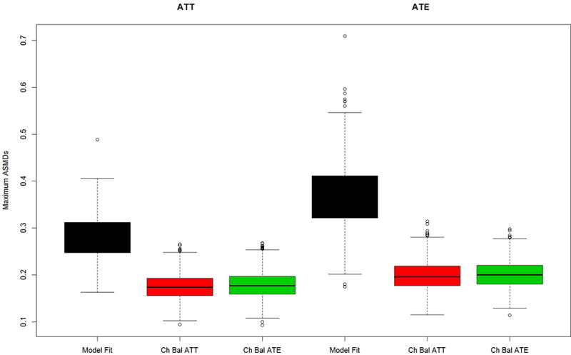
Figures 2 through 4 show box plots for the maximum ASMD for the four pretreatment covariates in propensity score Model A for the “no distractors”, “distractors”, and “all important” scenarios, respectively. For each scenario, we present results for both of our two different data generating models (PA and abstainers), and for each of the two possible estimands of interest ATT and ATE. For the chasing balance methods, results are shown for the stopping rule which yielded the smallest RMSE for that method (see appendix Tables A1 and A2 for the RMSEs for all stopping rules by method and scenario).

Figure 2.

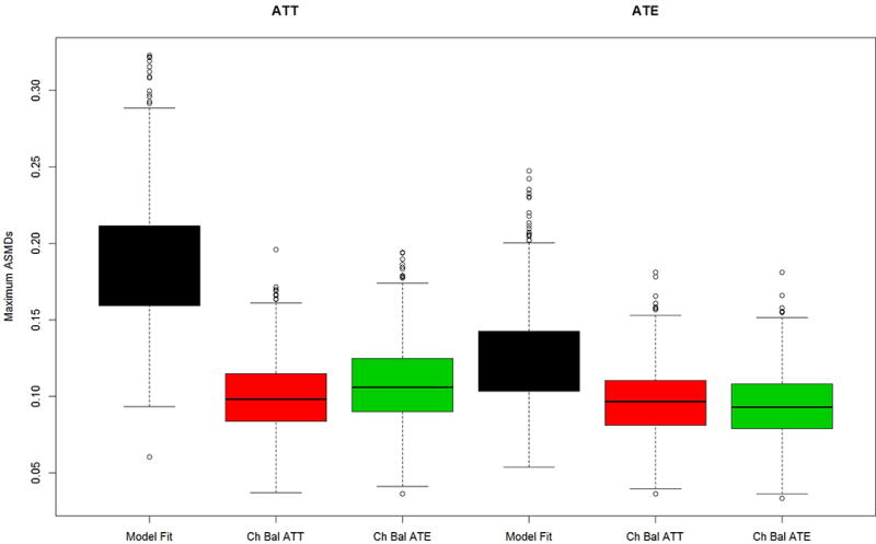
Maximum mean ASMD for Model A data generation and four covariates used in propensity score estimation (no distractors case) for (a) the PA and (b) the abstainers data generation case studies.

Figure 4.

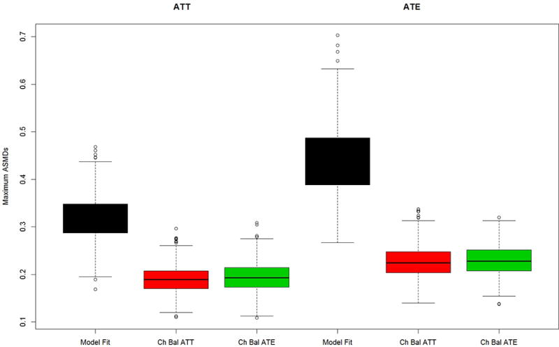
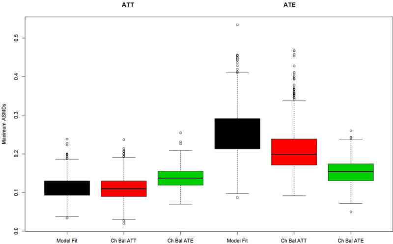
Maximum mean ASMD for Model B data generation and Model B propensity score estimation (All important case) for 4 most influential covariates for (a) the PA and (b) the abstainers data generation case studies.

Figures 2a and b present results for the two simulated case study settings, Case 1: PA vs. non-PA in 2a and Case 2: abstainers vs. users in 2b, for the “no distractors” scenario in which only 4 pretreatment variables matter and they are the only variables used in the propensity score estimation. Chasing balance on ATT or ATE performs well in terms of balance with maximum ASMDs generally well below 0.20, regardless of whether the estimated treatment is ATE or ATT. In all cases, using model fit to tune the GBM performs notably worse than either of the chasing balance approaches with a nearly 25% chance that the maximum ASMD would exceed 0.30 when estimating ATE for Case 2 (Figure 2b). Additionally, in both case studies chasing balance on ATT tends to slightly outperform chasing balance on ATE when interest lies in estimating ATTs and chasing balance on ATE achieves substantially better balance than chasing balance on ATT for the Case 2 when interest lies in ATE (See Figure 2b).

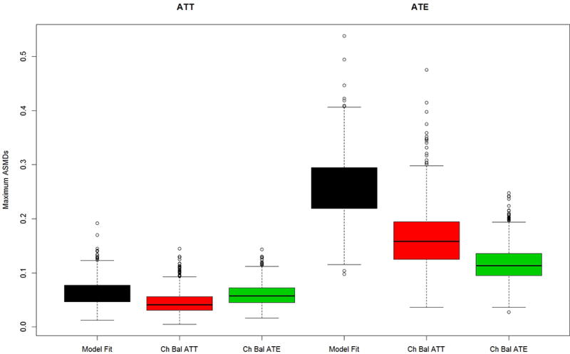
Figure 3 presents the results for the distractor scenario in which extraneous variables were used to estimate the propensity scores the same four pretreatment covariates as shown in Figures 2. Comparing the results from Figure 3 to those of Figure 2, shows that including distractors in the propensity score estimation results in larger values for the maximum ASMDs than modeling without them, regardless of the method used to tune the GBM model. The relative performances of the alternative methods for selecting the optimal GBM generally follow the patterns in Figure 2. In Case 1 (Figure 3a), chasing ATE balance or chasing ATT balance leads to similarly good balance, regardless of the estimand of interest. Model fit yields significantly worse balance in all cases expect in Case 2 (Figure 3b) when interest lies in ATT, in which case it performs about equally well as chasing balance. Moreover, for Case 2 when interest lies in ATE both model fit and chasing balance on ATT yield much worse balance in comparison to the method which chases ATE balance.

Figure 3.

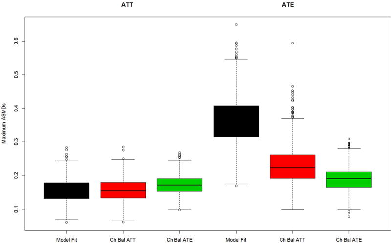
Maximum mean ASMD for Model A data generation but with all covariates used in propensity score estimation (distractors case) for (a) the PA and (b) the abstainers data generation case studies

Figures 4 a and b present the maximum ASMD for the same four pretreatment covariates as shown in Figures 2 and 3, for the “all important” scenario in which all the variables were used for estimating and generating the true propensity scores as well as being related to the outcome. Note the four covariates from our no distractors and distractors cases remain the most influential, even though all covariates contribute to the true propensity scores. As shown in Figures 4a and b, when the true propensity score model contains 47 or 90 covariates the maximum ASMDs for the four most influential covariates increase relative to the “no distractors” case in which the propensity score models depend on only 4 covariates, but the results are generally similar to those shown in Figures 3a and 3b (the “distractors” case). That is, modeling the propensity score with more covariates increases the maximum ASMD, regardless of whether or not all the covariates truly belong in the model. The story for comparing methods for choosing the optimal iteration of the GBM fit again replicates the findings from the other two scenarios: Model fit continues to yield weights that perform poorly at balancing, except for Case 2 when the estimand is ATT, in which case the methods perform similarly. Also, the two chasing balance methods perform similarly in all cases except Case 2 when interest lies in ATE; in that setting, chasing balance on ATE significantly outperforms model fit and chasing balance on ATT (the estimand that is not of primary interest).

Impact on Treatment Effect Estimation

Table 1 shows the standardized bias of the treatment effect, standard deviation, and RMSE for our treatment effect estimates for all of the scenarios, methods, and estimands of interest. For the chasing balance methods, results are shown for the stopping rule that produced optimal performance of the method with regard to RMSE. Appendix Table A1 and A2 shows the results for all stopping rules in detail and emphasizes how in any given setting the stopping rule that performed best varied.

Table 1.

Summary Statistics for Treatment Effect Estimates Across All Cases and Methods.

Case 1. PA (Treatment) vs. non-PA (Control)
		ATT			ATE
		Bias	Std Dev	RMSE	Bias	Std Dev	RMSE
No Distractors
Best Model Fit		0.068	0.042	0.080	0.004	0.022	0.022
Chasing Balance on ATT		0.061	0.041	0.073	0.012	0.022	0.025
Chasing Balance on ATE		0.059	0.041	0.072	0.008	0.022	0.023
Distractors
Best Model Fit		0.103	0.037	0.110	0.058	0.025	0.063
Chasing Balance on ATT		0.086	0.037	0.094	0.033	0.022	0.039
Chasing Balance on ATE		0.085	0.038	0.093	0.032	0.022	0.039
All Important
Best Model Fit		0.055	0.064	0.084	0.347	0.070	0.353
Chasing Balance on ATT		0.048	0.063	0.079	0.201	0.045	0.206
Chasing Balance on ATE		0.048	0.063	0.079	0.198	0.045	0.203
Case 2. Abstainers (Treatment) vs. Drug Users (Control)
No Distractors
Best Model Fit		0.035	0.058	0.068	0.494	0.105	0.505
Chasing Balance on ATT		0.001	0.054	0.054	0.313	0.096	0.327
Chasing Balance on ATE		−0.041	0.060	0.072	0.220	0.052	0.226
Distractors
Best Model Fit		−0.046	0.067	0.081	0.618	0.114	0.628
Chasing Balance on ATT		−0.041	0.066	0.078	0.376	0.101	0.390
Chasing Balance on ATE		−0.064	0.063	0.090	0.285	0.059	0.291
All Important
Best Model Fit		−0.086	0.088	0.124	0.538	0.123	0.552
Chasing Balance on ATT		−0.076	0.092	0.119	0.434	0.132	0.453
Chasing Balance on ATE		−0.119	0.089	0.147	0.285	0.059	0.291

Note: The true ATE = 0 in all cases while the true ATT = $761.36 and 9.66 for the abstainers and PA case studies, respectively (e.g, 0.25 times the observed standard deviation of the outcome in those datasets).

In the no distractor scenario, all three methods perform very similarly to each other for Case 1 when interest lies in either ATT or ATE. There is more separation between the methods for the Case 2. Here, when interest lies in ATT, we see that chasing balance on ATT slightly outperforms the other methods (RMSE equals 0.054 relative to 0.072 and 0.068 for chasing balance on ATE and model fit, respectively). Conversely, when interest lies in ATE, chasing balance on ATE clearly outperforms the alternatives (RMSE equals 0.226 relative to 0.327 and 0.505 for chasing balance on ATT and model fit, respectively). Notably, all methods result in biased treatment effect estimates for ATE in Case 2 (standardized bias is above 0.22 for all methods). This occurs because it is not feasible to obtain ATE weights to the match the covariate distribution for abstainers to those of the overall population. However, chasing balance on ATE achieves substantially better balance, smaller bias, smaller standard deviation, and smaller RMSE in the resulting treatment effects than the other methods. The results cannot be trusted for inferences about the treatment effect, but the case clearly demonstrates the strength of chasing balance with the targeted estimand to remove group differences.

In the distractors and all important cases, we generally see similar findings, although it is a little easier to delineate between model fit and the chasing balance methods in most cases than it was in the no distractor case. For Case 1, the two chasing balance methods both slightly outperform model fit and perform similarly to each other no matter whether one is interested in ATT or ATE. In contrast, chasing balance methods have more separation in Case 2. When interest lies in ATT, we see that chasing balance on ATT for Case 2 again yields the lowest bias and the smallest RMSE but chasing balance on ATE actually performs worse than model fit. Also, chasing balance on ATE when interest lies in ATE in Case 2 yields optimal performance. RMSE for chasing balance on ATE here is 0.291 (versus 0.390 for chasing balance on ATT and 0.628 for model fit) in the “distractors” case and 0.291 (versus 0.453 and 0.552, respectively) in the “all important” case. Again for the case of ATE when we use the abstainers data generation model, we continue to see poor performance overall given the lack of balance.

In almost all cases, controlling for more covariates via the propensity score models and weights has detrimental effects on the performance of the treatment effect estimates, regardless of whether or not selection into treatment depends on those variables. Standardized bias, standard deviation and RMSE are typically greater for all methods for the distractor and all important scenarios than for the no distractors scenario. For example, in the PA data generation case study, standardized bias changes from being less than 0.10 in the “no distractors case” to being over 0.20 in the “all important” case when interest lies in ATE. The degradation in performance is to be expected given the poorer performance in balance for the distractor and all important scenarios relative to no distractors shown in Figures 2 to 4. Lack of balance results in confounding of the treatment effect estimate. Also, the balance varies more across realized samples which adds to variance in the estimated treatment effect: A sample with particularly bad balance will yield outlying treatment effect estimates. Notably, in both case studies, better balance and lower standardize bias is achieved when interest lies in ATT versus ATE for the “all important” case. Finally, we note that modeling with many covariates allows for spurious variability in the weights that does not improve balance but inflates the variability of weighted means.

A concern with any weighting is that highly variable weights, relative to their mean, can result in some observations being extremely influential and can potentially inflate the standard error of a weighted mean. We explored how the different criteria for tuning GBM affect the coefficient of variation (CV) of the weights (i.e., the ratio of the standard error of the weights to the mean) for the treatment and control group by calculating the average values across simulated samples for each simulation setting. Full results are in Appendix Table A3. The CV was largest for best model fit when interest lies in ATT and there are no distractors for both the PA and the abstainer cases (averages = 1.12 and 1.25, respectively). Notably, the mean CV was consistently smaller for ATE than for ATT estimands. For ATT, chasing balance yielded less variable weights with the average CV ranging from 2 to 24% smaller than for best model fit, except in the all important case for abstainers in which the average CV for chasing balance was 6% larger. For ATE, without distractors, the CV was generally about the same for the PA case study across all methods while for the abstainers case study, chasing balance on ATE yielded smaller average values for CV. With distractors, chasing balance, especially ATE balance, yielded more variable weights than best model fit. The same was true when all predictors were important for PA but not abstainers. Taken altogether with the results above, for ATT, chasing balance can achieve better balance and less bias, without increasing the variability in the weights. The same is true for ATE, when there are only four covariates, but with many covariates, chasing balance obtained better balance at the cost of more variable weights but not necessarily great standard errors for the estimated treatment effect.

Table 2 presents the results for the impact on inferences for the different approaches to tuning GBM. For chasing balance the stopping rule which yielded the worst coverage rate is reported for each simulation setting (results for all methods are shown in Table A4 and A5). The estimated standard errors tend to be somewhat more accurate for best model fit than chasing balance. However, for both model fit and chasing balance, the sandwich standard errors are almost always notably too large for both approaches to tuning GBM. The bias in the sandwich standard errors tends to be largest for conditions in which the weights substantially reduced large differences between the treatment and the control group as they did for ATT and ATE using chasing ATE balance in the abstainer case. This result is consistent with fact that the sandwich standard error estimator estimates the standard error of the treatment effect as the square root of the variance of the weighted treatment mean plus the variance of the weighted control group mean and effectively ignores the correlation between these two weighted means. However, when the weights achieve balance they effectively create a positive correlation between the estimated treatment and control group means, so the standard error estimator tends to be too large, particularly in cases when the weights remove large differences between groups. Because chasing balance tends to achieve better balance than model fit, the sandwich standard errors tend to have greater bias for chasing balance than model fit.

Table 2.

Summary Statistics for Standard Errors and Inferences All Cases and Methods.

Case 1. PA (Treatment) vs. non-PA (Control)
		ATT		ATE
		Relative Standard Error	Coverage Rate	Relative Standard Error	Coverage Rate
No Distractors
Best Model Fit		0.85	0.47	1.57	1.00
Chasing Balance on ATT		0.99	0.60	1.58	1.00
Chasing Balance on ATE		0.98	0.61	1.56	1.00
Distractors
Best Model Fit		0.97	0.19	1.38	0.68
Chasing Balance on ATT		1.04	0.36	1.58	0.95
Chasing Balance on ATE		1.04	0.35	1.59	0.95
All Important
Best Model Fit		1.19	0.93	1.21	0.00
Chasing Balance on ATT		1.20	0.93	1.86	0.17
Chasing Balance on ATE		1.21	0.93	1.85	0.17
Case 2. Abstainers (Treatment) vs. Drug Users (Control)
No Distractors
Best Model Fit		2.04	1.00	1.33	0.02
Chasing Balance on ATT		2.27	1.00	1.70	0.19
Chasing Balance on ATE		2.02	1.00	2.68	0.84
Distractors
Best Model Fit		1.64	0.99	1.04	0.00
Chasing Balance on ATT		1.78	0.99	0.82	0.00
Chasing Balance on ATE		1.81	0.99	2.06	0.19
All Important
Best Model Fit		1.58	0.98	1.15	0.01
Chasing Balance on ATT		1.57	0.98	0.97	0.00
Chasing Balance on ATE		1.64	0.95	2.21	0.35

Note: The relative standard error equals the ratio of the Monte Carlo average of the estimated standard errors to the Monte Carlo standard deviation of the estimated treatment effects.

Across all the simulation conditions, chasing balance tends to have better coverage than model fit. There are, however, several conditions where both methods have low coverage such as ATE for the abstainers, where the estimated treatment effects tend to have large bias and ATT for PA for the no-distractors and distractor cases. In these settings, although the bias is not large relative to the standard deviation of the outcome, it is large relative to the true standard error and the estimated standard errors are accurate for chasing balance. In other cases, such as ATT for the abstainers or ATE for PA with no distractors, both methods have very high coverage. This is the result of three factors: 1) the bias is relatively small; 2) achieving balance is difficult so the true standard errors are relatively large, so that bias is smaller relative to the standard error than in other cases such as ATT for PA; and 3) the estimated standard errors consistently have large positive bias which increase the confidence intervals widths and coverage rates.

5 Illustrative data analysis

5.1 PA vs non-PA

Table 3 shows the balance results and treatment effect estimates from applying our three methods for fine tuning GBM to the original PA versus non-PA example. Here, the propensity score models only included the four most influential pretreatment covariates that were used to generate Model A in our simulation studies (namely self-reported need for treatment (sum of 5 items), sum of number of problems paying attention, controlling their behavior or breaking rules, an indicator for needing treatment for marijuana use, and SFS). As expected, in both the ATT and ATE analyses, model fit does the worst at obtaining balance on the pretreatment covariates (max ASMD equals 0.21 in both cases). Here, both chasing balance methods perform similarly for ATT and ATE, yielding max ASMDs ranging from 0.13 to 0.15. In spite of these differences in balance for model fit and the other methods, the treatment effect estimates for the three methods are highly similar: Among the population assigned to PA, the treatment appears to reduce substance use relative to the other alternative placements the probationers might have received, although confidence intervals include zero. PA does not appear effective for youth who would typically not be assigned to it as the ATE is close to zero regardless of the method used to tune GBM.

Table 3.

ASMD for each pretreatment covariate and summary statistics across covariates as well as treatment effect estimates (standardized) for ATE and ATT analyses for each candidate approach to select optimal iteration of GBM for PA versus non-PA example

		Unweighted	Chasing balance on ATT	Chasing balance on ATE	Model Fit
ATE analysis
Need for tx		0.79	0.15	0.15	0.18
SFS		0.63	0.09	0.09	0.15
Sum of probs		0.08	0.02	0.02	0.02
Tx for mj		0.67	0.14	0.14	0.21
Mean ASMD		0.54	0.10	0.10	0.14
Max ASMD		0.79	0.15	0.15	0.21
TE (95% CI)		−0.31 (−0.51, −0.1)	−0.03 (−0.28, 0.22)	−0.03 (−0.28, 0.21)	−0.06 (−0.30, 0.18)
ATT Analysis
Need for tx		0.89	0.13	0.13	0.16
SFS		0.69	0.06	0.06	0.08
Sum of probs		0.09	0.06	0.04	0.01
Tx for mj		0.54	0.13	0.14	0.21
Mean ASMD		0.55	0.10	0.09	0.12
Max ASMD		0.89	0.13	0.14	0.21
TE		−0.31 (−0.51, −0.1)	−0.18 (−0.42, 0.05)	−0.17 (−0.4, 0.06)	−0.14 (−0.38, 0.09)

5.2 Abstainers vs drug users

Table 4 shows the balance results and treatment effect estimates from applying our three methods for fine-tuning GBM to the original abstainers versus drug users data. Here, the propensity score models only included the four most influential pretreatment covariates that were used to generate Model A in our simulation studies (namely SFS, SRS, IMDS and proportion of days in the past 90 the youth was drunk or high for most of the day) and we only utilized the maximum ASMD stopping rule. As expected given our simulation study, when interest lies in estimating ATE, the best balance is achieved by selecting the iteration of GBM that optimizes ATE balance while chasing balance on ATT and model fit do much worse (chasing balance on ATE has a maximum ASMD of 0.19 versus 0.36 and 0.26 for the other two methods, respectively). Similarly, when interest lies in estimating ATT, chasing balance on ATT clearly outperforms chasing balance on ATE and the model fit methods (max ASMD = 0.07, 0.14, 0.29, respectively). In spite of these differences in balance, the treatment effect estimates for the three methods are highly similar. For all three methods, the results of both the ATE and ATT analyses are also similar and suggest that abstaining from drugs for one year post-intake increases income 7-years later by 1.6 standard deviations. For ATT, the confidence intervals do not include zero, whereas for ATE confidence intervals include zero since the standard errors are larger because both groups are weighted and the weights are highly variable with the groups being highly disparate. The differential imbalance in the covariates across methods for tuning GBM does not affect the treatment effect estimates because the covariates are only weakly related to outcomes (multiple R-squared is less than 0.01).

Table 4.

ASMD for each pretreatment covariate and summary statistics across covariates as well as treatment effect estimates (standardized) for ATE and ATT analyses for each candidate approach to select optimal iteration of GBM for the abstainers versus drug users example

		Unweighted	Chasing balance on ATT	Chasing balance on ATE	Model Fit
ATE analysis
SFS		0.70	0.34	0.18	0.26
SRS		0.60	0.36	0.19	0.25
IMDS		0.15	0.12	0.15	0.17
Days high or drunk		0.62	0.28	0.15	0.24
Mean ASMD		0.52	0.27	0.17	0.23
Max ASMD		0.70	0.36	0.19	0.26
TE (95% CI)		1.55 (−0.04, 3.13)	1.85 (−0.33, 4.03)	1.59 (−0.13, 3.31)	1.48 (−0.14, 3.09)
ATT Analysis
SFS		1.01	0.02	0.10	0.25
SRS		0.64	0.02	0.06	0.17
IMDS		0.18	0.07	0.06	0.01
Days high or drunk		1.02	0.05	0.14	0.29
Mean ASMD		0.71	0.04	0.09	0.18
Max ASMD		1.02	0.07	0.14	0.29
TE		1.55 (−0.04, 3.13)	1.60 (−0.02, 3.22)	1.67 (0.07, 3.27)	1.66 (0.06, 3.25)

6 Discussion

In this paper, we examine two important issues regarding implementation of GBM to estimate propensity score weights: the criteria for tuning the GBM and impact of including irrelevant covariates (distractors) in the models. In terms of criteria of tuning the model, our findings regarding the performance of the best model fit approach versus chasing balance approaches relates to the theoretical result in the field that show modeling with estimated propensity scores yields more precise treatment effect estimates than modeling with the true propensity scores because the estimated propensity score adjust for the imbalances that are observed between the treatment groups being compared (Hirano, Imbens, and Ridder 2003). Thus, even though the best model fit approach produces estimated propensity scores that most closely line up with the “true” propensity score model (results available upon request), the estimated propensity scores that result from this type of optimization do not obtain the best balance between the treatment and control groups and hence in turn result in treatment effect estimates that have larger bias. We suspect overfitting helps to correct for small sample bias that prevents the GBM from fully recovering the true propensity score model. By overfitting using balance to tune the model, GBM fit via chasing balance better balances the pretreatment covariates and reduces bias. These findings also reinforce the point made by others (Westreich et al. 2011) that obtaining best model fit for a propensity score model does not correspond with how well it actually performs in bias reduction.

As expected, we found that including distrators in the GBM modeling degraded the balance achieved by the resulting weights and increased the RMSE of the estimated treatment effects, in all simulations studied. This finding is consistent with what others in the field have found (Brookhart et al. 2006, Wyss et al. 2013, Setodji et al. Submitted , Setodji et al. conditional acceptance ). Given that we include such a large number of variables into the model, it is notable that all of the methods still perform reasonably well in all cases where distractor variables are added into the model (maximum mean ASMDs and standardized bias in the treatment effect estimate are all below 0.11), except the ATE case in the abstainers data generation case study. We would not expect such high performance from a parametric approach like the logistic regression model. Thus, while we do not recommended including so many variables in a propensity score estimation model if some can be eliminated on substantive grounds, it is clear that machine learning techniques can handle a large number of pretreatment covariates (e.g., between 47 and 90) where traditional parametric models are likely to fail. We found the modeling with many variables related to both treatment and outcomes also degrades performance relative to modeling with a small number of relevant variables, suggesting a limit to how far GBM can be pushed with a moderately large sample size of 1000. Even with the rise of machine learning techniques in propensity score estimation, analysts and researchers should still be careful when selecting the number of variables to include in the propensity score model in order to help ensure the best results are achieved. Future work could examine settings in which a variable selection step might be necessary prior to utilizing a machine learning approach for propensity score estimation.

The results for inferences are less clear than those for the accuracy of the treatment effect point estimate. No method of tuning GBM clearly provides better coverage than the others. Three factors contribute to this finding. First, bias in the treatment effect estimates reduces the probability of coverage. Second, large true standard errors increase the probability of coverage and, third, overestimating the standard error further increases the probability of coverage. Although chasing balance results in smaller bias, failure to balance the groups can increase the true standard errors so that model fit can have smaller bias relative to true standard errors, which makes coverage more likely even though the magnitude of the bias is greater. In addition, the sandwich standard error estimator that ignores the estimation of the weights overestimates the standard errors further distorting the coverage rates. The bias in the standard errors tends to be somewhat larger for chasing balance than best fit, precisely because chasing balance better balances covariates and reduces bias in the treatment effect. However, if bias in the treatment effect is small then even if intervals do not include the true value, they will be close to the truth. For example, if the effect is zero, and bias is small but the intervals do not include zero the inference would still be that the effect is small. On the other hand, large bias may be misinterpreted. For example, a large point value may be interpreted as a large effect, even if the interval is large and includes small values. Thus, even though the results on coverage do not favor any tuning method, chasing balance may still be preferable because it yields more accurate point estimates.

The results of our simulation study clearly demonstrate the poor performance of the sandwich standard error estimator that does not account for estimating weights. However, in a limited simulation study using a subset of the PA no-distractor samples, bootstrap standard errors also substantially overestimated the standard error, sometimes by a greater amount than the sandwich. Additional work is needed to determine the cause of the bias in the bootstrap standard errors and for potential alternatives.

Findings from this work have important implications for the field. Various promising methods are now available to researchers interested in estimating causal treatment effects with propensity scores. For many of the available approaches, it may be possible to improve performance if more care is taken in how the methods are fine-tuned to select a solution. For example, use of the super learning method which simultaneously runs multiple machine learning methods (including GBM) to estimate propensity scores is currently fine-tuned to select as optimal the combination of machine learners that yields the best prediction (van der Laan 2014, Pirracchio, Petersen, and van der Laan 2015). It may be feasible to improve the already high performance of this method by fine-tuning it so it selects as optimal the combination of machine-learners that yields the best balance. Future work might examine whether there are gains to this type of fine-tuning for that methodology.

Additionally, findings from our work follow in line with much of where the field is headed when developing new methods for improving estimation of propensity scores. For example, Imai and Ratkovic (2014) specifically developed the Covariate Balance Propensity Score (CBPS) method to improve performance of the standard logistic regression model for estimating propensity scores by incorporating a balance penalty function into the way in which logistic regression models estimate the propensity score. In addition, Hainmuller (2012) and Graham et al. (2012) use entropy or exponential tilting weights that provide exact balance on the covariates. Moreover, the high-dimensional propensity score (hd-PS) algorithm which is an automated technique that examines thousands of covariates in the study population to select the most salient variables for use in the propensity score model uses a strategy for selecting the most salient variables that prioritizes for selection those variables that are associated with the outcome and most imbalanced between the treatment and control groups (Schneeweiss et al. 2009). Thus in general, our results here may extend beyond machine learning methods, to support our inference that propensity score estimation in general can be optimized through careful consideration of balance.

Appendix

Table A1.

Summary Statistics for Treatment Effect Estimates for all stopping rules and methods considered for the abstainers’ example

Abstainers (Treatment) vs. Drug Users (Control)
		ATT			ATE
		Bias	Std Dev	RMSE	Bias	Std Dev	RMSE
No Distractors
Best Model Fit		0.035	0.058	0.068	0.494	0.105	0.505
Chasing Balance on ATT
es.max		−0.007	0.057	0.058	0.313	0.096	0.327
es.mean		0.001	0.054	0.054	0.344	0.084	0.354
ks.max		−0.001	0.060	0.060	0.335	0.098	0.349
ks.mean		0.003	0.054	0.054	0.350	0.083	0.360
Chasing Balance on ATE
es.max		−0.046	0.061	0.076	0.223	0.053	0.229
es.mean		−0.048	0.060	0.077	0.220	0.052	0.226
ks.max		−0.046	0.061	0.076	0.222	0.053	0.228
ks.mean		−0.041	0.060	0.072	0.222	0.052	0.228
Distractors
Best Model Fit		−0.046	0.067	0.081	0.618	0.114	0.628
Chasing Balance on ATT
es.max		−0.045	0.068	0.081	0.604	0.198	0.636
es.mean		−0.041	0.066	0.078	0.702	0.158	0.719
ks.max		−0.049	0.063	0.080	0.376	0.101	0.390
ks.mean		−0.042	0.066	0.078	0.647	0.143	0.662
Chasing Balance on ATE
es.max		−0.067	0.063	0.092	0.299	0.061	0.305
es.mean		−0.066	0.062	0.090	0.291	0.057	0.296
ks.max		−0.073	0.062	0.096	0.285	0.059	0.291
ks.mean		−0.064	0.063	0.090	0.294	0.055	0.299
All Important
Best Model Fit		−0.086	0.088	0.124	0.538	0.123	0.552
Chasing Balance on ATT
es.max		−0.086	0.093	0.127	0.656	0.210	0.689
es.mean		−0.076	0.092	0.119	0.751	0.155	0.766
ks.max		−0.089	0.090	0.126	0.434	0.132	0.453
ks.mean		−0.076	0.091	0.119	0.677	0.144	0.692
Chasing Balance on ATE
es.max		−0.121	0.086	0.149	0.306	0.064	0.312
es.mean		−0.121	0.085	0.148	0.290	0.059	0.296
ks.max		−0.131	0.086	0.156	0.285	0.059	0.291
ks.mean		−0.119	0.086	0.147	0.293	0.058	0.299

Table A2.

Summary Statistics for Treatment Effect Estimates for all stopping rules and methods considered for the PA example

PA (Treatment) vs. non-PA (Control)
		ATT			ATE
		Bias	Std Dev	RMSE	Bias	Std Dev	RMSE
No Distractors
Best Model Fit		0.068	0.042	0.080	0.004	0.022	0.022
Chasing Balance on ATT
es.max		0.061	0.041	0.073	0.013	0.022	0.025
es.mean		0.061	0.041	0.074	0.013	0.022	0.025
ks.max		0.062	0.041	0.074	0.013	0.022	0.026
ks.mean		0.061	0.041	0.073	0.012	0.022	0.025
Chasing Balance on ATE
es.max		0.059	0.041	0.072	0.009	0.022	0.024
es.mean		0.059	0.042	0.072	0.009	0.022	0.024
ks.max		0.059	0.042	0.072	0.009	0.022	0.024
ks.mean		0.059	0.042	0.073	0.008	0.022	0.023
Distractors
Best Model Fit		0.103	0.037	0.110	0.058	0.025	0.063
Chasing Balance on ATT
es.max		0.086	0.037	0.094	0.033	0.022	0.039
es.mean		0.086	0.037	0.094	0.033	0.022	0.039
ks.max		0.087	0.037	0.094	0.033	0.022	0.039
ks.mean		0.086	0.037	0.094	0.033	0.022	0.039
Chasing Balance on ATE
es.max		0.087	0.037	0.095	0.032	0.022	0.039
es.mean		0.085	0.038	0.093	0.032	0.022	0.039
ks.max		0.088	0.037	0.095	0.032	0.022	0.039
ks.mean		0.085	0.038	0.093	0.032	0.022	0.039
All Important
Best Model Fit via cv.folds		0.055	0.064	0.084	0.347	0.070	0.353
Chasing Balance on ATT
es.max		0.052	0.063	0.081	0.205	0.045	0.209
es.mean		0.048	0.063	0.080	0.201	0.045	0.206
ks.max		0.053	0.063	0.082	0.206	0.044	0.211
ks.mean		0.048	0.063	0.079	0.201	0.045	0.206
Chasing Balance on ATE
es.max		0.053	0.063	0.083	0.203	0.044	0.208
es.mean		0.048	0.063	0.079	0.198	0.045	0.203
ks.max		0.055	0.063	0.083	0.205	0.044	0.210
ks.mean		0.048	0.063	0.079	0.198	0.045	0.203

Table A3.

The Average Coefficient of Variation (CV) of the Weights for All Cases and Methods.

		Case 1. PA Case Study			Case 2. Abstainers Case Study
		ATT	ATE- Control	ATE- Treated	ATT	ATE- Control	ATE- Treated
No Distractors
Best Model Fit		1.12	0.39	0.64	1.25	0.26	0.64
Chasing Balance on ATT
es.max		1.06	0.38	0.60	1.09	0.24	0.64
es.mean		1.05	0.38	0.59	1.12	0.24	0.64
ks.max		1.05	0.38	0.59	1.11	0.24	0.64
ks.mean		1.06	0.38	0.60	1.12	0.24	0.65
Chasing Balance on ATE
es.max		1.10	0.39	0.63	0.95	0.21	0.62
es.mean		1.11	0.39	0.63	0.94	0.21	0.62
ks.max		1.10	0.39	0.63	0.95	0.21	0.62
ks.mean		1.12	0.39	0.64	0.96	0.21	0.63
Distractors
Best Model Fit		0.96	0.22	0.47	0.95	0.13	0.46
Chasing Balance on ATT
es.max		0.87	0.29	0.50	0.94	0.12	0.43
es.mean		0.87	0.29	0.50	0.98	0.11	0.37
ks.max		0.86	0.29	0.50	0.84	0.16	0.55
ks.mean		0.88	0.29	0.51	0.96	0.12	0.42
Chasing Balance on ATE
es.max		0.85	0.29	0.50	0.76	0.15	0.54
es.mean		0.89	0.29	0.51	0.76	0.15	0.55
ks.max		0.84	0.29	0.49	0.74	0.15	0.54
ks.mean		0.90	0.29	0.52	0.77	0.16	0.55
All Important
Best Model Fit		0.98	0.19	0.42	0.79	0.12	0.44
Chasing Balance on ATT
es.max		0.87	0.29	0.50	0.84	0.10	0.34
es.mean		0.90	0.29	0.51	0.89	0.09	0.30
ks.max		0.86	0.28	0.49	0.74	0.13	0.45
ks.mean		0.90	0.29	0.51	0.86	0.11	0.36
Chasing Balance on ATE
es.max		0.85	0.28	0.49	0.62	0.13	0.44
es.mean		0.90	0.29	0.52	0.61	0.13	0.44
ks.max		0.84	0.28	0.49	0.59	0.12	0.43
ks.mean		0.90	0.29	0.52	0.62	0.13	0.44

Table A4.

Relative Standard errors and coverage rates for all stopping rules and methods considered for the abstainers example

Abstainers (Treatment) vs. Drug Users (Control)
		ATT		ATE
		Relative Standard Error	Coverage Rate	Relative Standard Error	Coverage Rate
No Distractors
Best Model Fit		2.04	1.00	1.33	0.02
Chasing Balance on ATT
es.max		2.12	1.00	1.47	0.39
es.mean		2.27	1.00	1.67	0.22
ks.max		2.03	1.00	1.44	0.31
ks.mean		2.23	1.00	1.70	0.19
Chasing Balance on ATE
es.max		1.99	1.00	2.67	0.84
es.mean		2.02	1.00	2.72	0.86
ks.max		1.98	1.00	2.68	0.84
ks.mean		2.02	1.00	2.70	0.85
Distractors
Best Model Fit		1.64	0.9 9	1.0 4	0.0 0
Chasing Balance on ATT
es.max		1.66	0.99	0.60	0.01
es.mean		1.70	1.00	0.73	0.00
ks.max		1.78	0.99	1.23	0.06
ks.mean		1.71	1.00	0.82	0.00
Chasing Balance on ATE
es.max		1.79	0.99	2.06	0.19
es.mean		1.81	0.99	2.23	0.23
ks.max		1.80	0.99	2.13	0.26
ks.mean		1.80	0.99	2.27	0.21
All Important
Best Model Fit		1.58	0.9 8	1.1 5	0.0 1
Chasing Balance on ATT
es.max		1.51	0.98	0.67	0.02
es.mean		1.54	0.98	0.90	0.00
ks.max		1.57	0.98	1.07	0.08
ks.mean		1.55	0.98	0.97	0.00
Chasing Balance on ATE
es.max		1.63	0.96	2.21	0.35
es.mean		1.65	0.97	2.42	0.44
ks.max		1.64	0.95	2.39	0.46
ks.mean		1.64	0.96	2.47	0.41

Table A5.

Relative Standard errors and coverage rates for all stopping rules and methods considered for the PA example

		ATT		ATE
		Relative Standard Error	Coverage Rate	Relative Standard Error	Coverage Rate
No Distractors
Best Model Fit		0.85	0.47	1.57	1.00
Chasing Balance on ATT
es.max		0.99	0.61	1.58	1.00
es.mean		0.99	0.60	1.58	1.00
ks.max		1.00	0.60	1.57	1.00
ks.mean		0.99	0.61	1.57	1.00
Chasing Balance on ATE
es.max		0.99	0.62	1.56	1.00
es.mean		0.99	0.62	1.56	1.00
ks.max		0.99	0.62	1.56	1.00
ks.mean		0.98	0.61	1.55	1.00
Distractors
Best Model Fit		0.9 7	0.1 9	1.3 8	0.6 8
Chasing Balance on ATT
es.max		1.03	0.37	1.58	0.95
es.mean		1.03	0.37	1.58	0.95
ks.max		1.04	0.36	1.58	0.95
ks.mean		1.04	0.37	1.58	0.95
Chasing Balance on ATE
es.max		1.04	0.36	1.59	0.95
es.mean		1.03	0.38	1.58	0.96
ks.max		1.04	0.35	1.59	0.95
ks.mean		1.03	0.38	1.58	0.95
All Important
Best Model Fit via cv.folds		1.1 9	0.9 3	1.2 1	0.0 0
Chasing Balance on ATT
es.max		1.20	0.94	1.85	0.18
es.mean		1.20	0.94	1.85	0.21
ks.max		1.20	0.93	1.86	0.17
ks.mean		1.20	0.94	1.86	0.20
Chasing Balance on ATE
es.max		1.20	0.93	1.87	0.18
es.mean		1.20	0.94	1.86	0.22
ks.max		1.21	0.93	1.85	0.17
ks.mean		1.20	0.95	1.86	0.22

References

- Breiman Leo. Random Forests. Machine Learning. 2001;45:5–32. [Google Scholar]
- Brookhart M Alan, Schneeweiss Sebastian, Rothman Kenneth J, Glynn Robert J, Avorn Jerry, Stürmer Til. Variable Selection for Propensity Score Model. American Journal of Epidemiology. 2006;163(12):1149–1156. doi: 10.1093/aje/kwj149. [DOI] [PMC free article] [PubMed] [Google Scholar]
- Burgette L, McCaffrey DF, Griffin BA. Propensity score estimation with boosted regression. In: Pan W, Bai H, editors. Propensity score analysis: Fundamentals, developments, and extensions. New York (NY): Guilford Press; 2015. [Google Scholar]
- Burgette Lane, McCaffrey Daniel F, Griffin Beth Ann. Propensity Score Estimation with Boosted Regression. In: Pan Wei, Bai Haiyan., editors. Propensity Score Analysis: Fundamentals and Developments. New York: Guildford Publications; in press. [Google Scholar]
- Conover WJ. Practical Nonparametric Statistics. Vol. 3. Wiley; 1999. [Google Scholar]
- Dennis Michael L. Global Appraisal of Individual Needs (GAIN) Administration guide for the GAIN and related measures. Bloomington, IL: Chestnut Health Systems; 1999. [Google Scholar]
- Dennis Michael L, Chan Ya-Fen, Funk Rodney R. Development and Validation of the GAIN Short Screener (GSS) for Internalizing, Externalizing and Substance Use Disorders and Crime/Violence Problems Among Adolescents and Adults. The American Journal on Addictions. 2006;15(Suppl 1):80–91. doi: 10.1080/10550490601006055. [DOI] [PMC free article] [PubMed] [Google Scholar]
- Dudoit S, van der Laan MJ. Asymptotics of cross-validated risk estimation in estimator selection and performance assessment. Statistical Methodology. 2005;2(2):131–154. doi: 10.1016/j.stamet.2005.02.003. [DOI] [Google Scholar]
- Graham Bryan S, De Xavier Pinto Cristine Campos, Egel Daniel. Inverse probability tilting for moment condition models with missing data. The Review of Economic Studies. 2012;79(3):1053–1079. [Google Scholar]
- Griffin Beth Ann, Ramchand Rajeev, Edelen Maria Orlando, McCaffrey Daniel F, Morral Andrew R. Associations Between Abstinence in Adolescence and Economic and Educational Outcomes Seven Years Later Among High-risk Youth. Drug and Alcohol Dependence. 2011;113(2–3):118–24. doi: 10.1016/j.drugalcdep.2010.07.014. [DOI] [PMC free article] [PubMed] [Google Scholar]
- Hainmueller Jens. Entropy Balancing for Causal Effects: A Multivariate Reweighting Method to produce Balanced Samples in Observational Studies. Political Analysis. 2012;20(1):25–46. [Google Scholar]
- Harder VS, Stuart EA, Anthony JC. Propensity score techniques and the assessment of measured covariate balance to test causal associations in psychological research. Psychol Methods. 2010;15(3):234–49. doi: 10.1037/a0019623. doi: 2010-18042-002 [pii] 10.1037/a0019623. [DOI] [PMC free article] [PubMed] [Google Scholar]
- Hill Jennifer L. Bayesian Nonparametric Modeling for Causal Inference. Journal of Computational and Graphical Statistics. 2011;20(1):217–240. doi: 10.1198/jcgs.2010.08162. [DOI] [Google Scholar]
- Hirano Keisuke, Imbens Guido W, Ridder Geert. Efficient Estimation of Average Treatment Effects Using the Estimated Propensity Score. Econometrica. 2003;71(4):1161–1189. doi: 10.1111/1468-0262.00442. [DOI] [Google Scholar]
- Hunter Sarah B, Ramchand Rajeev, Griffin Beth Ann, Suttorp Marika J, McCaffrey Daniel, Morral Andrew. The effectiveness of community-based delivery of an evidence-based treatment for adolescent substance use. Journal of substance abuse treatment. 2012;43(2):211–220. doi: 10.1016/j.jsat.2011.11.003. [DOI] [PMC free article] [PubMed] [Google Scholar]
- Imai Kosuke, Ratkovic Marc. Covariate balancing propensity score. Journal of the Royal Statistical Society: Series B (Statistical Methodology) 2014;76(1):243–263. doi: 10.1111/rssb.12027. [DOI] [Google Scholar]
- Lee BK, Lessler J, Stuart EA. Improving propensity score weighting using machine learning. Stat Med. 2010;29(3):337–46. doi: 10.1002/sim.3782. [DOI] [PMC free article] [PubMed] [Google Scholar]
- Liaw Andy, Wiener Matthew. Classification and Regression by Random Forest. R News. 2002;2(3):18–22. [Google Scholar]
- McCaffrey Daniel F, Ridgeway Greg, Morral Andrew R. Propensity score estimation with boosted regression for evaluating causal effects in observational studies. Psychological methods. 2004a;9(4):403. doi: 10.1037/1082-989X.9.4.403. [DOI] [PubMed] [Google Scholar]
- McCaffrey Daniel F, Ridgeway Greg, Morral Andrew R. Propensity Score Estimation with Boosted Regression for Evaluating Causal Effects in Observational Studies. Psychological Methods. 2004b;9(4):403–425. doi: 10.1037/1082-989X.9.4.403. [DOI] [PubMed] [Google Scholar]
- Morral Andrew R, McCaffrey DF, Ridgeway G. Effectiveness of Community-based Treatment for Substance-abusing Adolescents: 12-month Outcomes of Youths Entering Phoenix Academy or Alternative Probation Dispositions. Psychology of Addictive Behaviors. 2004;18(3):257–68. doi: 10.1037/0893-164X.18.3.257. [DOI] [PubMed] [Google Scholar]
- Natekin Alexey, Knoll Alois. Gradient boosting machines, a tutorial. Frontiers in neurorobotics. 2013:7. doi: 10.3389/fnbot.2013.00021. [DOI] [PMC free article] [PubMed] [Google Scholar]
- Pearl Judea. Causality: Models, Reasoning, and Inference. New York: Cambridge University Press; 2000. [Google Scholar]
- Pirracchio Romain, Petersen Maya L, van der Laan Mark. Improving Propensity Score Estimators’ Robustness to Model Misspecification Using Super Learner. American Journal of Epidemiology. 2015;181(2):108–119. doi: 10.1093/aje/kwu253. [DOI] [PMC free article] [PubMed] [Google Scholar]
- Ramchand R, Griffin BA, Suttorp M, Harris KM, Morral A. Using a cross-study design to assess the efficacy of motivational enhancement therapy-cognitive behavioral therapy 5 (MET/CBT5) in treating adolescents with cannabis-related disorders. J Stud Alcohol Drugs. 2011;72(3):380–9. doi: 10.15288/jsad.2011.72.380. [DOI] [PMC free article] [PubMed] [Google Scholar]
- Ridgeway Greg. The State of Boosting. Computing Science and Statistics. 1999;31:172–181. [Google Scholar]
- Ridgeway Greg. Generalized Boosted Models: A guide to the gbm package. 2007 http://www.saedsayad.com/docs/gbm2.pdf.
- Ridgeway Greg. [Accessed February 18, 2013];GBM 1.6-3.1 Package Manual. 2011 doi:10.1.1.151.4024. [Google Scholar]
- Ridgeway Greg, McCaffrey Daniel F, Morral Andrew R, Burgette Lane F, Griffin Beth Ann. [Accessed October 1, 2014];Toolkit for Weighting and Analysis of Nonequivalent Groups: A Tutorial for the Twang Package. 2014 [Google Scholar]
- Rubin Donald B. Using propensity scores to help design observational studies: application to tobacco litigation. Health Services & Outcomes Research Methodology. 2001;2:169–188. [Google Scholar]
- Rubin Donald B. On principles for modeling propensity scores in medical research. Pharmacoepidemiol Drug Saf. 2004;13(12):855–7. doi: 10.1002/pds.968. [DOI] [PubMed] [Google Scholar]
- Schneeweiss Sebastian, Rassen Jeremy A, Glynn Robert J, Avorn Jerry, Mogun Helen, Brookhart MAlan. High-dimensional propensity score adjustment in studies of treatment effects using health care claims data. Epidemiology. 2009;20(4):512–22. doi: 10.1097/EDE.0b013e3181a663cc. [DOI] [PMC free article] [PubMed] [Google Scholar]
- Schuler M, Griffin BA, Ramchand R, Almirall D, McCaffrey D. Effectiveness of Adolescent Substance Abuse Treatments: Is Biological Drug Testing Sufficient? Journal of Studies of Alcohol and Drugs. 2014;75:358–370. doi: 10.15288/jsad.2014.75.358. [DOI] [PMC free article] [PubMed] [Google Scholar]
- Setodji C, McCaffrey DF, Burgette L, Almirall D, Griffin BA. conditional acceptance The right tool for the job: choosing between covariate balancing and generalized boosted model propensity scores. Epidemiology. doi: 10.1097/EDE.0000000000000734. [DOI] [PMC free article] [PubMed] [Google Scholar]
- Setodji Claude M, Almirall Daniel, Burgette Lane, Griffin Beth Ann, McCaffrey Daniel F. An Evaluation of Model Complexity in Propensity Score Estimation Submitted. [Google Scholar]
- Sinisi Sandra E, Polley Eric C, Petersen Maya L, Rhee Soo-Yon, van der Laan Mark. Super Learning: An Application to the Prediction of HIV-1 Drug Resistance. Statistical Applications in Genetics and Molecular Biology. 2007;6(1):1–26. doi: 10.2202/1544-6115.1240. [DOI] [PMC free article] [PubMed] [Google Scholar]
- van der Laan Mark J. Targeted estimation of nuisance parameters to obtain valid statistical inference. The International Journal of Biostatistics. 2014;10(1):29–57. doi: 10.1515/ijb-2012-0038. [DOI] [PubMed] [Google Scholar]
- van der Laan MJ, Polley EC, Hubbard AE. Super Learner. Statistical Applications in Genetics and Molecular Biology. 2007;6(1):1544–6115. doi: 10.2202/1544-6115.1309. [DOI] [PubMed] [Google Scholar]
- van der Laan MJ, Dudoit S, van der Vaart A. The cross-validated adaptive epsilon-net estimator. Statistics & Risk Modeling. 2006;24(3):373–395. doi: 10.1524/stnd.2006.24.3.373. [DOI] [Google Scholar]
- Westreich Daniel, Cole Stephen R, Funk Michele Jonsson, Brookhart MAlan, Stürmer Til. The role of the c-statistic in variable selection for propensity score models. Pharmacoepidemiology and Drug Safety. 2011;20(3):317–320. doi: 10.1002/pds.2074. [DOI] [PMC free article] [PubMed] [Google Scholar]
- Wooldridge Jeffrey M. Econometric Analysis of Cross Section and Panel Data. Cambridge: MIT Press; 2002. [Google Scholar]
- Wyss Richard, Girman Cynthia J, LoCasale Robert J, Brookhart MAlan, Stürmer Til. Variable Selection for Propensity Score Models When Estimating Treatment Effects on Multiple Outcomes: A simulation study. Pharmacoepidemiology and Drug Safety. 2013;22(1):77–85. doi: 10.1002/pds.3356. [DOI] [PMC free article] [PubMed] [Google Scholar]