Machine Learning in Medicine

Abstract

Spurred by advances in processing power, memory, storage, and an unprecedented wealth of data, computers are being asked to tackle increasingly complex learning tasks, often with astonishing success. Computers have now mastered a popular variant of poker, learned the laws of physics from experimental data, and become experts in video games – tasks which would have been deemed impossible not too long ago. In parallel, the number of companies centered on applying complex data analysis to varying industries has exploded, and it is thus unsurprising that some analytic companies are turning attention to problems in healthcare. The purpose of this review is to explore what problems in medicine might benefit from such learning approaches and use examples from the literature to introduce basic concepts in machine learning. It is important to note that seemingly large enough medical data sets and adequate learning algorithms have been available for many decades – and yet, although there are thousands of papers applying machine learning algorithms to medical data, very few have contributed meaningfully to clinical care. This lack of impact stands in stark contrast to the enormous relevance of machine learning to many other industries. Thus part of my effort will be to identify what obstacles there may be to changing the practice of medicine through statistical learning approaches, and discuss how these might be overcome.

Machine learning is the scientific discipline that focuses on how computers learn from data^4,5. It arises at the intersection of statistics, which seeks to learn relationships from data, and computer science, with its emphasis on efficient computing algorithms. This marriage between mathematics and computer science is driven by the unique computational challenges of building statistical models from massive data sets, which can include billions or trillions of data points. The types of learning used by computers are conveniently subclassified into categories such as supervised learning and unsupervised learning. However, I find, in addition, that another division can be useful when considering how machine learning might inform the practice of medicine: distinguishing learning those tasks that physicians can already do well and learning those where physicians have had only limited success. With these broad categories in mind, we can visit some areas in medicine that have benefited or might benefit from machine learning approaches.

Supervised learning

Supervised learning starts with the goal of predicting a known output or target. In machine learning competitions, where individual participants are judged on their performance on common data sets, recurrent supervised learning problems include handwriting recognition (such as recognizing handwritten digits), classifying images of objects (e.g. is this a cat or a dog?), and document classification (e.g. is this a clinical trial about heart failure or a financial report?). Notably, these are all tasks that a trained person can do well and so the computer is often trying to approximate human performance. Supervised learning focuses on classification, which involves choosing among subgroups to best describe a new data instance, and prediction, which involves estimating an unknown parameter (such as the temperature in San Francisco tomorrow afternoon).

What might be some examples of supervised learning in medicine? Perhaps the most common example seen by a cardiologist is the automated interpretation of the EKG, where pattern recognition is performed to select from a limited set of diagnoses (i.e. a classification task). In radiology, automated detection of a lung nodule from a chest X-ray would also represent supervised learning. In both these cases, the computer is approximating what a trained physician is already capable of doing with high accuracy.

Supervised learning is often used to estimate risk. The Framingham Risk Score³ for coronary heart disease (CHD) may in fact be the most commonly used instance of supervised learning in medicine. Such risk models exist across medicine, and include guiding antithrombotic therapy in atrial fibrillation⁴ and implantation of automated implantable defibrillators in hypertrophic cardiomyopathy⁵. In modeling risk, the computer is doing more than merely approximating physician skills but finding novel relationships not readily apparent to human beings.

Unsupervised learning

In contrast, in unsupervised learning, there are no outputs to predict. Instead, we are trying to find naturally occurring patterns or groupings within the data. This is inherently a more challenging task to judge and often the value of such groups learned through unsupervised learning is evaluated by its performance in subsequent supervised learning tasks (i.e. are these new patterns useful in some way?).

When might such approaches be used in medicine? Perhaps the most compelling opportunity represents the “precision medicine” initiative⁶. Frustrated by the inherent heterogeneity in most common diseases, there is a growing effort to redefine disease according to pathophysiologic mechanisms, which could, in turn, provide new paths to therapy. But identifying such mechanisms for complex multifactorial diseases will not be easy. Let us think about how one might apply unsupervised learning in cardiac disease towards that end, taking a heterogeneous condition like myocarditis. One can start with a large group of apparently similar individuals with unexplained acute systolic heart failure. One can then perform myocardial biopsies on them, and characterize the cellular composition of each sample with a technique such as immunostaining. For example, one would have a tally of T lymphocytes, neutrophils, macrophages, eosinophils, etc. One could then see if there are recurring patterns of cellular composition, which, in turn, might suggest mechanism and guide therapies to explore. A similar approach, albeit focused on genomics, led to identifying an eosinophilic subtype of asthma⁷, which uniquely responds to a novel therapy targeting the eosinophil-secreted cytokine IL-13⁸. Note the contrast with supervised learning – there is no predicted outcome – we are only interested in identifying patterns in the data. In fact, treating this as a supervised learning problem – such as developing a model of mortality in myocarditis and classifying patients by risk – might miss such subgroups completely, thereby losing a chance to identify novel disease mechanisms.

The learning problem

Let us now define the learning problem more generally in order to understand why complex machine learning algorithms have had such a limited presence in actual clinical practice. I will focus first on supervised learning and address unsupervised learning at a later point.

We will take as our goal the prediction of MI and for simplicity treat this as a classification problem, with individuals who have had one or more MIs as one class and (age and gender matched) individuals free of MI as a second class (Figure 1A). Our assignment, then, is to build an accurate model to discriminate between the two classes. The first task is to come up with some predictors or features. Some obvious features include hypertension, diabetes and LDL-cholesterol level. But how did we come up with these, and how can we expand this pool further? A simple way would be to test candidate predictors for association with heart attack status and keep only those that are significant. But this will miss a great number of features that might be useful only within a subset of heart attack patients. Worse yet, there may be features that are useful in combinations (of two, three, or more) but not on their own. As a solution, we might be tempted to give up and throw in all possible features, but instinctively, we have some suspicion that this might not help or may even make things worse (for reasons that will become apparent later). “Feature selection” is the area of machine learning that focuses on this problem⁹.

Figure 1.

Machine learning overview. A. Matrix representation of the supervised and unsupervised learning problem. We are interested in developing a model for predicting myocardial infarction (MI). For training data, we have patients, each characterized by an outcome (positive or negative training examples), denoted by the circle in the right-hand column, as well as by values of predictive features, denoted by blue to red coloring of squares. We seek to build a model to predict outcome using some combination of features. Multiple types of functions can be used for mapping features to outcome (B–D). Machine learning algorithms are used to find optimal values of free parameters in the model in order to minimize training error as judged by the difference between predicted values from our model and actual values. In the unsupervised learning problem, we are ignoring the outcome column, and grouping together patients based on similarities in the values of their features. B. Decision trees map features to outcome. At each node or branch point, training examples are partitioned based on the value of a particular feature. Additional branches are introduced with the goal of completely separating positive and negative training examples. C. Neural networks predict outcome based on transformed representations of features. A hidden layer of nodes integrates the value of multiple input nodes (raw features) to derive transformed features. The output node then uses values of these transformed features in a model to predict outcome. D. The k-nearest neighbor algorithm assigns class based on the values of the most similar training examples. The distance between patients is computed based on comparing multidimensional vectors of feature values. In this case, where there are only two features, if we consider the outcome class of the three nearest neighbors, the unknown data instance would be assigned a “no MI” class.

The next challenge is to come up with a function that relates values of the features to a prediction of disease (class assignment). This challenge can be broken down into two steps. First we need to decide on which type of function we want to work with (Figure 1B–D). Classical statistics would have us consider the logistic regression model for this task. With logistic regression, a type of generalized linear model, features come into the model additively and linearly. But this is only one possible class of function and if we relax this assumption, many more choices exist. For example decision trees could be used to predict heart attack status, allowing the flexibility of “OR” choices (Figure 1B). A heart attack patient might have mutually exclusive causes such as familial hypercholesterolemia OR an arterial thrombotic disorder OR HIV, which would be difficult to model with logistic regression. Other types of machine learning models such as neural networks allow transformations of input features to better predict outcomes (Figure 1C). Support vector machines build classification models using a transformed set of features in much higher dimensions¹⁰. Prototype methods, such as k-nearest neighbors do away with the idea of building a model, and instead make predictions based on the outcome of similar case examples¹¹ (Figure 1D). The best guess for whether our patient will have a heart attack is to see if similar patients tend to have heart attacks.

All of these choices of functional classes have free parameters to fit. In logistic regression, the regression coefficients – that is the weights applied to individual features – need to be determined. In decision trees, one has to choose the variables at which a split is performed and in the case of quantitative variables, the values at which the split is made. Neural networks have free parameters related to the function used for feature transformation, as well as the function used to predict class based on these derived features. Finding optimal values for these free parameters is a daunting task. Machine learning algorithms represent computational methods to efficiently navigate the space of free parameters to arrive at a good model. Note the distinction between algorithms, which consist of instructions followed by the computer to complete a particular task, and models, which are derived from the application of algorithms to data.

How do we fit these free parameters? And, more importantly, how do we tell that we’re doing a good job? Machine learning tries to separate these tasks, focusing on a training set of examples to perform such tasks as feature selection and parameter fitting, and a test set to evaluate model performance. Using the training examples, we can try out different values for the free parameters and assess how similar our predicted outputs are to the known outputs – this is sometimes called estimating "training error” and one uses a “loss function” that is tailored to reflect what sort of errors are more tolerable than others. We want a model that minimizes training error and our chosen algorithm fits free parameters to achieve this goal.

A high-performing model requires multiple attributes for success. First of all, you need informative features that actually reflect how the classes are different from another. For tasks that we already know humans can do well, we know that we have the requisite input data. For example, if the goal is to approximate the ability of an expert cardiologist to read an ECG, we can be confident that the ECG itself includes all the features that are needed for a correct classification. But for more challenging classification problems, such as discriminating MI cases from controls, our limited understanding of disease pathogenesis makes it unlikely that we are collecting all of the information needed for accurate classification.

Even if we are collecting the requisite inputs, we still need some function to combine them to achieve the desired task. For complex learning tasks, we might need considerable flexibility in how the features are used, as simple additive models are unlikely to achieve an effective separation between cases and not controls. One often speaks about how “expressive” a certain class of functions, which typically involves some transformation or higher order combination of features to carry out complex learning tasks.

We have described two interdependent attributes – informative features and expressive functions – to achieve low training error. But minimizing training error is not enough. Really, what we would like to be able to do is to make excellent predictions/classifications for individuals we've never seen before. To assess this generalization ability, we should save some data that we've never looked at to evaluate our "test error”. Such test data should not have been used for any aspect of the machine learning process, including feature selection or data normalization. Ideally, we would like to feel confident that if we have built a model with low training error, we will have some guarantee that it also has low test error. Otherwise we might be falsely and perhaps dangerously impressed by our own predictive ability.

A considerable amount of theory exists for machine learning that establishes bounds for similarity between training error and test error¹⁰. Although the mathematics is elaborate, the message is quite simple: models that are highly complex (including those that have a large number of features) may do better at minimizing training error, but tend to generalize poorly for a given number of training samples as they tend to overfit to the data. A corollary to this is if you need a high amount of model complexity in order to make accurate predictions on your training set, you will need many, many more training examples to ensure that you generalize well to previously unseen individuals.

A tradeoff thus exists between complexity of the model and generalizability to new data sets. One solution is to simply have fewer features and a less expressive model. But in this case, we may be harming ourselves with a low quality model with poor accuracy on the training set. As an alternative, machine learning experts continue to use flexible models but penalize themselves for too much complexity such as having too many free parameters or allowing too broad a range of values for these parameters – a process known as “regularization”. This may mean that accuracy on the training set might suffer a little, but the benefit will be better performance on test data.

Given the diverse menu of machine learning algorithms and data models, can we find some guidance on which would work best in one situation or another? As a rule of thumb, the best solution would involve fitting a model that matches the underlying model that generated the data. Unfortunately, we typically have no idea what that underlying model is. An empiric solution is to try a number of algorithms, making sure to keep aside test data on which to evaluate performance. But that can be time consuming, especially if some approaches are unlikely to work well a priori. Many machine-learning practitioners have a toolkit of feature extraction and preprocessing approaches as well as a subset of supervised and unsupervised learning algorithms that they feel very comfortable with and return to. When training data is limited, these often include simpler models with regularization such as penalized forms of linear and logistic regression. These might not lead to as low training error as complex models (the term high bias is used) but they tend to generalize well (low variance). When training data are abundant and the underlying model is likely to arise from non-additivity and complex interactions between features, instance approaches like k-nearest neighbors or decision tree algorithms (such as stochastic gradient tree boosting^12,13 or random forest¹⁴, discussed below) can work well. Some algorithms such as non-linear support vector machines¹⁵ can be extremely robust in a variety of situations even where the number of predictive features is very large compared to the number of training examples, a situation where over-fitting often occurs. Finally, accepting the limitations of each class of algorithms, some practitioners use a process called blending, merging the outputs of multiple different algorithms (also discussed below).

Finally, for challenging prediction problems, it means that considerable effort needs to be made to amass as many training examples as possible, all characterized by the same set of informative features. If one examines the amount of training data that is used in image analysis competitions – which can include over 100,000 images – we see that the typical biomedical data sets fall short by two to three orders of magnitude, despite representing arguably a fundamentally more challenging learning task. And this deficiency in amount of training data does not even begin to address the fact that we typically have no idea what features are needed to capture the complexity of the disease process. It is primarily this challenge – collecting many thousands if not tens of thousands of training examples all characterized by a rich set of (sufficiently) informative features, that has limited the contribution of machine learning to complex tasks of classification and prediction in clinical medicine.

Illustrative examples of machine learning

To illustrate some of the points addressed here, I will focus on four examples of machine learning in medicine, covering a range of supervised and unsupervised approaches. Two of these focus on cardiovascular disease and two on cancer.

Supervised learning – learning from forests and trees

Although a tremendous number of supervised learning algorithms have been developed, their goals are shared: to provide sufficient flexibility to minimize training error but at the same time allow generalization to new data sets, all in a computationally efficient way. I highlight one of these methods – random forests – as an example of an innovative and highly effective algorithm.

The random forests algorithm, developed nearly 15 years ago¹⁴, is touted as one of the best “off-the-shelf” algorithms for classification available. As their name would suggest, random forests are constructed from trees – more specifically decision trees. Let us assume that the goal is to classify individuals into two groups – such as statin responders or non-responders. We start with a group of training examples consisting of known statin responders and non-responders, each characterized by a set of features, such as age, sex, and smoking and diabetes status. Often hundreds or thousands of features may be available. We build a series (“ensemble”) of decision trees that each seek to use these predictive features to discriminate between our two groups. At each node in each tree, one feature is selected that most effectively achieves this split. Since it is unlikely that a single variable will be sufficient, subsequent nodes are then needed to achieve a more perfect separation. A notable difference between each tree is that each only has access to a subset of training examples – a concept known as “bagging”¹⁶. Furthermore, at each node, only a subset of features is considered. The resulting stochasticity allows each tree to cast an independent vote on a final classification and serves as a means of regularization. Even though each tree is unlikely to be accurate on its own, the final majority vote across hundreds of trees is remarkably accurate.

Random forests have had incredible success across a variety of learning disciplines and have fared well in machine learning competitions. Ishwaran, Lauer and colleagues adapted random forests to the analysis of survival data – and aptly termed their approach “random survival forests (RSF)”¹⁷. They used a binary variable for death and applied their method to a variety of problems, including prediction of survival in systolic heart failure¹⁸ and in postmenopausal women¹⁹. In the latter example they looked at 33,144 women in the Women’s Health Initiative Trials and considered conventional clinical and demographic variables as well as 477 ECG biomarkers. They used RSF to build a survival model – and identified 20 variables predictive of long-term mortality, including 14 ECG biomarkers. Models constructed using this reduced subset of features demonstrated improved performance, both on training data and on a held out test set. Interestingly, once the subset of 20 variables were selected, a simple additive model (a regularized version of the Cox proportional hazards model) performed just as well as RSF in patient classification, suggesting that one of the main merits of RSF was in feature selection. Many of these variables had in fact never before been implicated in predicting mortality.

Why hasn’t this approach been replicated and incorporated into prevalent risk models? The primary reason may be that the RSF performance was actually inferior to that typically seen with the commonly used Framingham Risk Score, despite the fact that the latter involves fewer variables and a simpler model²⁰. How could that be? Although the large sample size was enviable compared to most epidemiological studies, it came at a price. Many variables were by self-report and most blood biomarkers were absent, presumably because the cost of performing detailed phenotyping on such a large cohort would be prohibitive. Notably absent were cholesterol measures, including total cholesterol and LDL-cholesterol. The authors were also unable to find an external data set for replication, because few cohorts had the same quantitative ECG variables measured. Thus despite representing a novel application of a superb algorithm, the study’s benefits were limited by not having training and test data sets with a common comprehensive set of informative features, including all those previously found to be important for this prediction task.

C-Path: an automated pathologist and the importance of feature extraction

As highlighted above, feature selection is central to machine learning. Without adequate informative predictors, we are unlikely to make progress, despite sophisticated algorithms. A recent example from the field of breast cancer pathology is particularly illustrative of when machine learning approaches might succeed and when they are unlikely to add benefit to current conventional clinical practices.

Koller and colleagues at Stanford University focused on improving identification of high risk breast cancer cases using pathological specimens – developing a tool called C-Path²¹ (Figure 2). Many of the unfavorable histologic properties of tumors used today such as tubules and atypical nuclei had been identified decades ago. However, rather than simply combine these using new algorithms, C-Path took a further step back and focused on identifying new features using automated image processing. C-Path first developed a classifier that could robustly differentiate between the epithelial and stromal portions of the tumor (Figure 2A–B). It then derived a rich quantitative feature set of 6642 predictors from these regions examined separately and together, highlighting epithelial and stromal “objects” and their relationships, such as properties of nuclei (size, location, spacing) and relationships between nuclei and cytoplasm in epithelium and stroma (Figure 2C). These features were then used to construct a model to predict survival, which demonstrated excellent performance on two independent test data sets, superior to that achieved by community pathologists. Furthermore, the C-Path scores were significantly associated with 5-year survival above and beyond all established clinical and molecular factors (Figure 2D).

Figure 2.

Overview of the C-Path image processing pipeline and prognostic model building procedure. A. Basic image processing and feature construction. B. Building an epithelial-stromal classifier. The classifier takes as input a set of breast cancer microscopic images that have undergone basic image processing and feature construction and that have had a subset of superpixels hand-labeled by a pathologist as epithelium(red) or stroma (green). The superpixel labels and feature measurements are used as input to a supervised learning algorithm to build an epithelial-stromal classifier. The classifier is then applied to new images to classify superpixels as epithelium or stroma. C. Constructing higher-level contextual/relational features. After application of the epithelial stromal classifier, all image objects are subclassified and colored on the basis of their tissue region and basic cellular morphologic properties. (Left panel) After the classification of each image object, a rich feature set is constructed. D. Learning an image-based model to predict survival. Processed images from patients alive at 5 years after surgery and from patients deceased at 5 years after surgery were used to construct an image-based prognostic model. After construction of the model, it was applied to a test set of breast cancer images (not used in model building) to classify patients as high or low risk of death by 5 years. From Beck et al, Sci Transl Med. 2011;3:108ra113. Reprinted with permission from AAAS.

The C-Path experience was instructive for several reasons. Perhaps the most important lesson was that novel learned features were essential to improved performance – one could not simply dress up established features in a new algorithmic packaging and expect superior classification. Moreover, many of the predictive features learned by C-Path were entirely novel despite decades of examination of breast cancer slides by pathologists. Thus one of the main contributions of machine learning is to take an unbiased approach to identify unexpected informative variables. The second lesson to be learned is that the final algorithm used for classification, a regularized form of logistic regression called “lasso”²², was actually quite simple but still generated excellent results. Simple algorithms can perform just as well as more complex ones in two circumstances: when the underlying relationship between features and output is simple (e.g. additive) or when the number of training examples is low, and thus more complex models are likely to overfit and generalize poorly. If one truly needs the benefits of more complex models such as those capturing high-dimensional interactions, one should focus on amassing sufficient and diverse training data to have any hope of building an effective classifier. Finally, the C-Path authors found that the success of their model crucially depended on being able to first differentiate epithelium and stroma. As it is unlikely that a machine would arrive at the need for this step on its own, this highlights the need for domain-specific human expertise to guide the learning process.

Although analysis of pathology samples plays a limited role in clinical cardiology, one can imagine extrapolating this approach of data-driven feature extraction to other information rich types, such as cardiac MRI images or electrograms.

Attractor metagenes in cancer and bake-offs in machine learning

A second machine learning example in cancer biology is illustrative of the interplay between unsupervised and supervised learning and introduces the concept of “blending” to improve predictive models.

Given the abundance of learning algorithms and the fact that some approaches are more suited to particular problems, the machine learning community has embraced the idea of competitions. In these algorithm “bake-offs”, multiple individuals or groups are given the same training data and asked to develop predictive models, which in turn are evaluated on an independent test set. A particularly high profile version of this was the $1,000,000 Netflix Grand Prize^23,24, where money was awarded to the group that could most improve the prediction of movie preferences based on past ratings. Such competitions have had a tremendously beneficial impact on the machine learning field, including ensuring transparency and reproducibility, encouraging sharing of methods, and avoiding the danger of investigators retrospectively “adjusting” an analysis to arrive at the desired result. Similar competitions have appeared within the biology community²⁵ – but are rare in medical research, where data sets and methods are not routinely shared.

The recent Sage Bionetworks-DREAM Breast Cancer Prognosis Challenge (BCC) exemplifies the promise of this type of approach for clinical medicine²⁶. BCC represented an open challenge to build predictive models for breast cancer based on genomic, clinical, and survival outcome data from nearly 2000 patients. Over 350 groups from 35 countries participated and generated predictive models for survival outcomes, which were evaluated on a newly generated validation set of 184 patients. Interestingly, the winning model²⁷ was built in part from genomic features identified through applying unsupervised learning to completely unrelated cancers. The authors had previously developed an algorithm known as “attractor metagenes”²⁸, which identified clusters of genes that shared similarity across multiple tumor samples. Many of these clusters happened to correspond to biological processes essential for cancer progression such as “chromosomal instability” and “mesenchymal transition”. The authors incorporated the presence or absence of these features along with other clinical variables into various predictive models for breast cancer outcomes. Since different learning algorithms may be more or less effective for predicting outcomes for specific types of patients, the authors used several different supervised learning algorithms and performed a blending of each algorithm’s output into a final prediction of survival outcomes (Figure 3).

Figure 3.

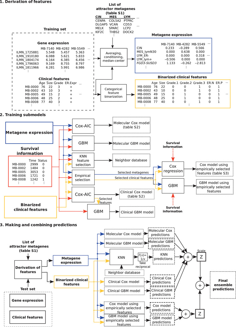
Schematic of model development for breast cancer risk prediction. Shown are block diagrams that describe the development stages for the final ensemble prognostic model. Building a prognostic model involves derivation of relevant features, training submodels and making predictions, and combining predictions from each submodel. The model derived the attractor metagenes using gene expression data, combined them with the clinical information through Cox regression, gradient boosting machine, and k-nearest neighbor techniques, and eventually blended each submodel’s prediction. From Cheng et al, Sci Transl Med. 2013;5:181ra50. Reprinted with permission from AAAS.

Several instructive aspects emerged from this competition. The first is that unsupervised learning can be seen as a means of feature selection, as it can allow discovery of robust biological descriptors, which can then be used in a supervised model for disease prediction. The second lesson is that an ensemble of different learning algorithms was able to produce a superior prediction than any single one alone. Thirdly, models using both genomic and clinical variables ended up surpassing either data type alone. Finally, learning benefited from having nearly 2000 data sets for training and validation as well as a transparent framework that allowed sharing of code and gave participants constant feedback on their performance.

Unsupervised learning in HFpEF: towards precision medicine?

Heart failure with preserved ejection fraction (HFpEF) is a highly heterogeneous condition with no proven therapies²⁹. One possibility for the lack of successful clinical trials in HFpEF is that enrolled patients reflect multiple dominant pathophysiologic processes, not all of which would respond to the same agent. Can such processes be identified? Although some have suggested using genetics for precise redefinition of diseases, genetic variation is unlikely to help classify complex conditions like HFpEF, where it is most probable that hundreds of weak genetic factors interact with each other and the environment in an unpredictable way to elicit disease phenotypes.

We focused on using unsupervised learning for classifying HFpEF patients. As mentioned above, unsupervised learning seeks to find internal structure in the data. It starts from a similar framework as supervised learning, with instances (patients in this case) each characterized by a feature vector, where values are given for particular attributes such as height, sex and age. These data can be conveniently represented by a matrix (Figure 1A). But instead of using this matrix to learn a model relating features to outcomes, we instead use it to find group of patients that are similar to one another. Multiple algorithms can be used for this purpose. Perhaps the simplest is agglomerative hierarchical clustering, which first groups together individuals that are most similar to one another, and then merges together similar pairs, and so on and so on. Another class of unsupervised learning algorithms, including principal component analysis and non–negative matrix factorization³⁰, performs a matrix decomposition, converting the patient-feature matrix into a product of two matrices: one which groups together similar features into super-features (we call this dimensionality reduction) and a second which describes each patient by a vector of weights applied to these super-features. Patients would then be grouped based on similarity of their weight vectors. Another set of unsupervised learning methods such as k-medoids clustering³¹ and the attractor metagenes algorithm²⁸ try to find distinct training examples (or a composite) around which to group other data instances. Examples within a cluster should be more similar to each other than to those of other clusters.

Sparse coding represents a recent advance to the field of unsupervised learning. It was originally devised to assist in the field of computer vision³², which involves the automated acquisition, processing and interpretation of images, and focuses on such tasks as facial recognition and the interpretation of handwritten text. Sparse coding is believed to reflect the way in which the visual cortex responds to stimuli. Rather than have a large number of cortical neurons activated by every image, the principle of sparsity instead has a very small number of neurons attuned to a much more specific, higher order aspect of the image, such as the edge of an object oriented in a particular direction. Algorithmic improvements allow computers to learn a set of such higher order features from training images and then interpret test images as a composite of these features³³. With enough training data, computers can perform such complex tasks as distinguishing between different food types (https://www.metamind.io/vision/food). In addition to image recognition, sparse coding has been applied successfully to natural language processing³⁴. We will later discuss if such approaches might be of use in patient classification for the purposes of precision medicine.

In our analysis of HFpEF, we were interested in grouping patients on the basis of quantitative echocardiographic and clinical variables³⁵. Starting with 67 diverse features, we removed highly correlated features to leave 46 minimally redundant predictors (Figure 4A). We used a regularized form of model-based clustering, where multivariate Gaussian distributions were used to define each patient cluster on the basis of the means and standard deviation assigned to each feature. To achieve parsimony, regularization was used to select the optimal number of patient clusters as well as the number of free parameters fit in defining each cluster (Figure 4B). Patients were assigned to clusters based on computing a joint probability across all features and choosing the cluster with the highest probability of membership for each patient. Comparison of the resulting groups demonstrated differences across a wide range of phenotypic variables. Similar to the BCC prize winner, we used our phenotypic clusters as features in a supervised learning model to predict survival of HFpEF patients and found that they improved upon the clinical models commonly used for risk assessment, both within our training set and in an independent test set (Figure 4C).

Figure 4.

Application of unsupervised learning to HFpEF. A. Phenotype heat map of HFpEF. Columns represent individual study participants; rows, individual features. B. Bayesian information criterion analysis for the identification of the optimal number of phenotypic clusters (pheno-groups). C. Survival free of cardiovascular (CV) hospitalization or death stratified by phenotypic cluster. Kaplan-Meier curves for the combined outcome of heart failure hospitalization, cardiovascular hospitalization, or death stratified by phenotypic cluster.

Needless to say this is only a start. Utility of any such classification should be validated in survival models in other cohorts, especially because cluster definitions are all too dependent on which features are chosen and which learning algorithm is used. More importantly, we would like to use such classification to revisit failed clinical trials in HFpEF such as TOPCAT³⁶ to see if any of the groups we defined would identify a subclass of patients who might benefit from specific therapies.

Discussion

Based on the above examples it is obvious that machine learning – both supervised and unsupervised – can be applied to clinical data sets for the purpose of developing robust risk models and redefining patient classes. This is unsurprising, as problems across a broad range of fields, from finance to astronomy to biology¹³, can be readily reduced to the task of predicting outcome from diverse features or finding recurring patterns within multidimensional data sets. Medicine should not be an exception. However, given the limited clinical footprint of machine learning, some obstacles must be standing in the way of translation.

Some of these may relate to pragmatic issues relevant to the medical industry, including reimbursement and liability. For example, our health system is reluctant to completely entrust a machine with a task that a human can do at higher accuracy, even if there is substantial cost savings. For machine learning to be incorporated in areas where it cannot promise as high accuracy as that of a human expert, there must be ways for physicians to interact with computer systems to maintain accuracy and yet increase throughput and reduce cost. For example, one can imagine an automated system that errs on the side of very high sensitivity and uses human over-reading to increase specificity. A new reimbursement model for such an integrated man-and-machine approach will be needed. And physicians will need to become comfortable with the risks of medical error – which may be no greater than in other clinical circumstances – but nonetheless may feel different because of the “black box” nature of the automated system. On-site evaluation with local data for a sufficiently long trial period may alleviate some of those concerns. And if we place increasing reliance on stand-alone highly accurate expert systems to lower medical costs, will the makers of these systems assume any liability?

An unrelated challenge is whether an FDA clinical indication will be granted to a drug for a subgroup of patients that has been defined in a manner unrelated to the mechanism of action of that drug. While it is straightforward to target a specific kinase inhibitor towards cancer patients with an activating driver mutation in that same kinase, it is not clear how, for example, we could justify matching our HFpEF classes with a particular type of drug, no matter how phenotypically homogeneous the group may be. Empirical evidence of disproportionate therapeutic benefit in one class over another would be necessary – but is it sufficient? I suspect this inability to justify matching a patient subgroup to a drug on a biological basis will represent an inherent challenge to the reclassification of most complex diseases, as these typically cannot be defined by genetics alone or an obvious biomarker linked to the drug’s therapeutic mechanism. As a solution, clinical trials could be adequately powered for all predefined subgroups but it remains to be seen what evidence would be needed for a subgroup-selective drug approval.

Some difficulties in the adoption of machine learning in medicine may also be related to actual statistical challenges in learning. Towards that point, we can extract a number of useful lessons from the examples I highlighted as well as the broader experiences of the machine learning community. First of all, novel informative features will be needed to build improved models in medicine, particularly in learning situations where the computer is not simply approximating the physician’s performance. Merely using the same predictors with more innovative algorithms is unlikely to add much value. In the case of C-Path, features were derived through automated image analysis, while in the attractor metagenes algorithm, they arose from genomic analyses of tumors. In both cases, the potential pool of new features was in the tens of thousands.

For cardiovascular disease, where the tissue of interest is not readily accessible, it will be challenging to find large unbiased sources of phenotypic data with sufficient informativeness to characterize the disease process. In our study of the HFpEF patients, we used echocardiographic data. Likewise other features could come from noninvasive characterization of myocardial tissue and vascular beds. Some even hope that mobile devices may offer a lower cost, detailed phenotypic characterization of patients³⁷. It remains to be seen if the information content of data from imaging or mobile recording modalities will match that of genomic (or proteomic or metabolomic) data, with the caveat that, in the case of cardiac patients, such ‘omic data may have to come from peripheral blood and not from the myocardium or vasculature. In this regard, we are at a disadvantage relative to oncology. It is difficult to see a path forward for deriving biologically rich features in the absence of obtaining cardiac or vascular tissue, unless, we can somehow develop safe perturbational agents to probe specific pathway activities within these inaccessible organs, which can then be quantified through imaging³⁸.

To be in a position to extract novel features, we must somehow find the appetite to collect large amounts of unbiased data on many thousands of individuals without knowing that such an effort will actually be useful. And it won’t be enough to collect such data on the training cohort alone. As the RSF experience demonstrated, it is essential that the same informative features in any promising model be collected on multiple independent cohorts for them to serve as test sets. Unfortunately, such biologically informative features are likely to be costly to acquire (unlike the tens of thousands of digital snapshots of cats used as training data in image processing applications³⁹).

The final lesson is a technical one, related to the interplay of unsupervised and supervised forms of learning. Deep learning, with stacked layers of increasingly higher order representations of objects, has taken the machine learning world by storm⁴⁰. Deep learning uses unsupervised learning to first find robust features, which can then be refined, and ultimately used as predictors in a final supervised model. Our work³⁵ and that involving attractor metagenes²⁷ both suggest that such techniques might be useful for patient data. In a deep learning representation of human disease, lower layers could represent clinical measurements (such as ECG data or protein biomarkers), intermediate layers could represent aberrant pathways (which may simultaneously impact many biomarkers), and top layers could represent disease subclasses (which arise from the variable contributions of one or more aberrant pathways). Ideally such subclasses would do more than stratify by risk, and actually reflect the dominant disease mechanism(s). This raises a question about the underlying pathophysiologic basis of complex disease in any given individual: is it sparsely encoded in a limited set of aberrant pathways, which could be recovered by an unsupervised learning process (albeit with the right features collected and a large enough sample size), or is it a diffuse, multifactorial process with hundreds of small determinants combining in a highly variable way in different individuals? In the latter case, the concept of “precision medicine” is unlikely to be of much utility. However, in the former situation, unsupervised and perhaps deep learning might actually realize the elusive goal of reclassifying patients according to more homogenous subgroups, with shared pathophysiology, and the potential of shared response to therapy.

References

- 1.Hastie T, Tibshirani R, Friedman J. The Elements of Statistical Learning. New York, NY: Springer Science & Business Media; 2009. [Google Scholar]
- 2.Abu-Mostafa YS, Magdon-Ismail M, Lin H-T. Learning from Data. 2012 AMLbook.com. [Google Scholar]
- 3.Kannel WB, Doyle JT, McNamara PM, Quickenton P, Gordon T. Precursors of sudden coronary death. Factors related to the incidence of sudden death. Circulation. 1975;51:606–613. doi: 10.1161/01.cir.51.4.606. [DOI] [PubMed] [Google Scholar]
- 4.Lip GYH, Nieuwlaat R, Pisters R, Lane DA, Crijns HJGM. Refining clinical risk stratification for predicting stroke and thromboembolism in atrial fibrillation using a novel risk factor-based approach: the euro heart survey on atrial fibrillation. Chest. 2010;137:263–272. doi: 10.1378/chest.09-1584. [DOI] [PubMed] [Google Scholar]
- 5.O'Mahony C, Jichi F, Pavlou M, Monserrat L, Anastasakis A, Rapezzi C, Biagini E, Gimeno JR, Limongelli G, McKenna WJ, Omar RZ, Elliott PM. A novel clinical risk prediction model for sudden cardiac death in hypertrophic cardiomyopathy (HCM risk-SCD) Eur Heart J. 2014;35:2010–2020. doi: 10.1093/eurheartj/eht439. [DOI] [PubMed] [Google Scholar]
- 6.National Research Council (US) Committee on A Framework for Developing a New Taxonomy of Disease. Toward Precision Medicine: Building a Knowledge Network for Biomedical Research and a New Taxonomy of Disease. Washington (DC): National Academies Press (US); 2011. [PubMed] [Google Scholar]
- 7.Woodruff PG, Modrek B, Choy DF, Jia G, Abbas AR, Ellwanger A, Koth LL, Arron JR, Fahy JV. T-helper type 2-driven inflammation defines major subphenotypes of asthma. Am J Respir Crit Care Med. 2009;180:388–395. doi: 10.1164/rccm.200903-0392OC. [DOI] [PMC free article] [PubMed] [Google Scholar]
- 8.Corren J, Lemanske RF, Hanania NA, Korenblat PE, Parsey MV, Arron JR, Harris JM, Scheerens H, Wu LC, Su Z, Mosesova S, Eisner MD, Bohen SP, Matthews JG. Lebrikizumab treatment in adults with asthma. N Engl J Med. 2011;365:1088–1098. doi: 10.1056/NEJMoa1106469. [DOI] [PubMed] [Google Scholar]
- 9.Guyon I, Elisseeff A. An introduction to variable and feature selection. J Mach Learn Res. 2003;3:1157–1182. [Google Scholar]
- 10.Vapnik VN. An overview of statistical learning theory. IEEE Trans Neural Netw. 1999;10:988–999. doi: 10.1109/72.788640. [DOI] [PubMed] [Google Scholar]
- 11.Cover T, Hart P. Nearest neighbor pattern classification. IEEE Trans Inf Theory. 1967;13:21–27. [Google Scholar]
- 12.Friedman JH. Greedy function approximation: A gradient boosting machine. Ann Statist. 2001;29:1189–1232. [Google Scholar]
- 13.Deo RC, Musso G, Taşan M, Tang P, Poon A, Yuan C, Felix JF, Vasan RS, Beroukhim R, De Marco T, Kwok P-Y, Macrae CA, Roth FP. Prioritizing causal disease genes using unbiased genomic features. Genome Biol. 2014;15:534. doi: 10.1186/s13059-014-0534-8. [DOI] [PMC free article] [PubMed] [Google Scholar]
- 14.Breiman L. Random forests. Mach Learn. 2001;45:5–32. [Google Scholar]
- 15.Burges CJ. A tutorial on support vector machines for pattern recognition. Data Min Knowl Discov. 1998;2:121–167. [Google Scholar]
- 16.Breiman L. Bagging predictors. Mach Learn. 1996;24:123–140. [Google Scholar]
- 17.Ishwaran H, Kogalur UB, Lauer MS. Random survival forests. Ann Appl Stat. 2008;2:841–860. [Google Scholar]
- 18.Hsich E, Gorodeski EZ, Blackstone EH, Ishwaran H, Lauer MS. Identifying important risk factors for survival in patient with systolic heart failure using random survival forests. Circ Cardiovasc Qual Outcomes. 2011;4:39–45. doi: 10.1161/CIRCOUTCOMES.110.939371. [DOI] [PMC free article] [PubMed] [Google Scholar]
- 19.Gorodeski EZ, Ishwaran H, Kogalur UB, Blackstone EH, Hsich E, Zhang Z-M, Vitolins MZ, Manson JE, Curb JD, Martin LW, Prineas RJ, Lauer MS. Use of hundreds of electrocardiographic biomarkers for prediction of mortality in postmenopausal women: the Women's Health Initiative. Circ Cardiovasc Qual Outcomes. 2011;4:521–532. doi: 10.1161/CIRCOUTCOMES.110.959023. [DOI] [PMC free article] [PubMed] [Google Scholar]
- 20.d'Agostino RB, Sr, Grundy S, Sullivan LM, Wilson P. Validation of the Framingham Coronary Heart Disease Prediction Scores. JAMA. 2001;286:180–187. doi: 10.1001/jama.286.2.180. [DOI] [PubMed] [Google Scholar]
- 21.Beck AH, Sangoi AR, Leung S, Marinelli RJ, Nielsen TO, van de Vijver MJ, West RB, van de Rijn M, Koller D. Systematic analysis of breast cancer morphology uncovers stromal features associated with survival. Sci Transl Med. 2011;3:108ra113–108ra113. doi: 10.1126/scitranslmed.3002564. [DOI] [PubMed] [Google Scholar]
- 22.Tibshirani R. Regression Shrinkage and Selection via the Lasso. J R Stat Soc Series B Stat Methodol. 1996;58:267–288. [Google Scholar]
- 23.Koren Y. The bellkor solution to the netflix grand prize. Netflix prize documentation. 2009 [Google Scholar]
- 24.Töscher A, Jahrer M, Bell RM. The bigchaos solution to the netflix grand prize. Netflix prize documentation. 2009 [Google Scholar]
- 25.Peña-Castillo L, Taşan M, Myers CL, Lee H, Joshi T, Zhang C, Guan Y, Leone M, Pagnani A, Kim WK, Krumpelman C, Tian W, Obozinski G, Qi Y, Mostafavi S, Lin GN, Berriz GF, Gibbons FD, Lanckriet G, Qiu J, Grant C, Barutcuoglu Z, Hill DP, Warde-Farley D, Grouios C, Ray D, Blake JA, Deng M, Jordan MI, Noble WS, Morris Q, Klein-Seetharaman J, Bar-Joseph Z, Chen T, Sun F, Troyanskaya OG, Xu D, Hughes TR, Roth FP. A critical assessment of Mus musculus gene function prediction using integrated genomic evidence. Genome Biol. 2008;9(Suppl 1):S2. doi: 10.1186/gb-2008-9-s1-s2. [DOI] [PMC free article] [PubMed] [Google Scholar]
- 26.Margolin AA, Bilal E, Huang E, Norman TC, Ottestad L, Mecham BH, Sauerwine B, Kellen MR, Mangravite LM, Furia MD, Vollan HKM, Rueda OM, Guinney J, Deflaux NA, Hoff B, Schildwachter X, Russnes HG, Park D, Vang VO, Pirtle T, Youseff L, Citro C, Curtis C, Kristensen VN, Hellerstein J, Friend SH, Stolovitzky G, Aparicio S, Caldas C, Borresen-Dale AL. Systematic Analysis of Challenge-Driven Improvements in Molecular Prognostic Models for Breast Cancer. Sci Transl Med. 2013;5:181re1–181re1. doi: 10.1126/scitranslmed.3006112. [DOI] [PMC free article] [PubMed] [Google Scholar]
- 27.Cheng WY, Yang THO, Anastassiou D. Development of a Prognostic Model for Breast Cancer Survival in an Open Challenge Environment. Sci Transl Med. 2013;5:181ra50. doi: 10.1126/scitranslmed.3005974. [DOI] [PubMed] [Google Scholar]
- 28.Cheng W-Y, Ou Yang T-H, Anastassiou D. Biomolecular events in cancer revealed by attractor metagenes. PLoS Comput Biol. 2013;9:e1002920. doi: 10.1371/journal.pcbi.1002920. [DOI] [PMC free article] [PubMed] [Google Scholar]
- 29.Udelson JE. Heart Failure With Preserved Ejection Fraction. Circulation. 2011;124:e540–e543. doi: 10.1161/CIRCULATIONAHA.111.071696. [DOI] [PubMed] [Google Scholar]
- 30.Lee DD, Seung HS. Learning the parts of objects by non-negative matrix factorization. Nature. 1999;401:788–791. doi: 10.1038/44565. [DOI] [PubMed] [Google Scholar]
- 31.Kaufman L, Rousseeuw P. Reports of the Faculty of Mathematics and Informatics. 87. Delft: Faculty of Mathematics and Informatics; 1987. Clustering by Means of Medoids. Part 3. [Google Scholar]
- 32.Olshausen BA, Field DJ. Sparse coding with an overcomplete basis set: a strategy employed by V1? Vision Res. 1997;37:3311–3325. doi: 10.1016/s0042-6989(97)00169-7. [DOI] [PubMed] [Google Scholar]
- 33.Lee H, Battle A, Raina R, Ng A. Efficient sparse coding algorithms. Advances in Neural Information Processing Systems. 2007 [Google Scholar]
- 34.Yogatama D, Faruqui M, Dyer C, Smith NA. Learning Word Representations with Hierarchical Sparse Coding. CORD Conference Proceedings. 2014 [Google Scholar]
- 35.Shah SJ, Katz DH, Selvaraj S, Burke MA, Yancy CW, Gheorghiade M, Bonow RO, Huang C-C, Deo RC. Phenomapping for novel classification of heart failure with preserved ejection fraction. Circulation. 2015;131:269–279. doi: 10.1161/CIRCULATIONAHA.114.010637. [DOI] [PMC free article] [PubMed] [Google Scholar]
- 36.Pitt B, Pfeffer MA, Assmann SF, Boineau R, Anand IS, Claggett B, Clausell N, Desai AS, Diaz R, Fleg JL, Gordeev I, Harty B, Heitner JF, Kenwood CT, Lewis EF, O'Meara E, Probstfield JL, Shaburishvili T, Shah SJ, Solomon SD, Sweitzer NK, Yang S, McKinlay SM TOPCAT Investigators. Spironolactone for heart failure with preserved ejection fraction. N Engl J Med. 2014;370:1383–1392. doi: 10.1056/NEJMoa1313731. [DOI] [PubMed] [Google Scholar]
- 37.Ausiello D, Shaw S. Quantitative human phenotyping: the next frontier in medicine. Trans Am Clin Climatol Assoc. 2014;125:219–226. discussion 226–8. [PMC free article] [PubMed] [Google Scholar]
- 38.James ML, Gambhir SS. A Molecular Imaging Primer: Modalities, Imaging Agents, and Applications. Physiol Rev. 2012;92:897–965. doi: 10.1152/physrev.00049.2010. [DOI] [PubMed] [Google Scholar]
- 39.Le QV. Building high-level features using large scale unsupervised learning; ICASSP 2013 - 2013 IEEE International Conference on Acoustics, Speech and Signal Processing (ICASSP); 2013. pp. 8595–8598. [Google Scholar]
- 40.Bengio Y. Learning deep architectures for AI. FNT in Machine Learning. 2009;2:1–127. [Google Scholar]
Associated Data
This section collects any data citations, data availability statements, or supplementary materials included in this article.