Multi‐site quality and variability analysis of 3D FDG PET segmentations based on phantom and clinical image data

Abstract

Purpose

Radiomics utilizes a large number of image‐derived features for quantifying tumor characteristics that can in turn be correlated with response and prognosis. Unfortunately, extraction and analysis of such image‐based features is subject to measurement variability and bias. The challenge for radiomics is particularly acute in Positron Emission Tomography (PET) where limited resolution, a high noise component related to the limited stochastic nature of the raw data, and the wide variety of reconstruction options confound quantitative feature metrics. Extracted feature quality is also affected by tumor segmentation methods used to define regions over which to calculate features, making it challenging to produce consistent radiomics analysis results across multiple institutions that use different segmentation algorithms in their PET image analysis. Understanding each element contributing to these inconsistencies in quantitative image feature and metric generation is paramount for ultimate utilization of these methods in multi‐institutional trials and clinical oncology decision making.

Methods

To assess segmentation quality and consistency at the multi‐institutional level, we conducted a study of seven institutional members of the National Cancer Institute Quantitative Imaging Network. For the study, members were asked to segment a common set of phantom PET scans acquired over a range of imaging conditions as well as a second set of head and neck cancer (HNC) PET scans. Segmentations were generated at each institution using their preferred approach. In addition, participants were asked to repeat segmentations with a time interval between initial and repeat segmentation. This procedure resulted in overall 806 phantom insert and 641 lesion segmentations. Subsequently, the volume was computed from the segmentations and compared to the corresponding reference volume by means of statistical analysis.

Results

On the two test sets (phantom and HNC PET scans), the performance of the seven segmentation approaches was as follows. On the phantom test set, the mean relative volume errors ranged from 29.9 to 87.8% of the ground truth reference volumes, and the repeat difference for each institution ranged between −36.4 to 39.9%. On the HNC test set, the mean relative volume error ranged between −50.5 to 701.5%, and the repeat difference for each institution ranged between −37.7 to 31.5%. In addition, performance measures per phantom insert/lesion size categories are given in the paper. On phantom data, regression analysis resulted in coefficient of variation (CV) components of 42.5% for scanners, 26.8% for institutional approaches, 21.1% for repeated segmentations, 14.3% for relative contrasts, 5.3% for count statistics (acquisition times), and 0.0% for repeated scans. Analysis showed that the CV components for approaches and repeated segmentations were significantly larger on the HNC test set with increases by 112.7% and 102.4%, respectively.

Conclusion

Analysis results underline the importance of PET scanner reconstruction harmonization and imaging protocol standardization for quantification of lesion volumes. In addition, to enable a distributed multi‐site analysis of FDG PET images, harmonization of analysis approaches and operator training in combination with highly automated segmentation methods seems to be advisable. Future work will focus on quantifying the impact of segmentation variation on radiomics system performance.

1. Background

Radiomics is an emerging discipline that utilizes quantitative image‐derived features for predicting both underlying molecular and genetic characteristics as well as clinical response and outcomes. These features can thereby be used to facilitate clinical decision making and treatment selection as a key component of personalized cancer treatment.^{1, 2} FDG PET imaging is an established and effective tool for tumor burden quantification, also known as metabolic tumor volume (MTV).^{3, 4, 5} Measurement of tumor volume is frequently utilized in radiomics, and is made even more critical, because feature extraction is often dependent upon analysis of the voxels that lie inside the defined volume.

At minimum, several steps are required to generate such FDG PET based volumes and features, including image acquisition, reconstruction, and lesion segmentation. Clearly, the quality (i.e., predictive power) of the image‐derived features depends on the quality and consistency of the individual steps. Currently, there are several efforts underway to standardize and harmonize PET scanner performance. These efforts include standardization of patient preparation and image acquisition,^{6, 7, 8} as well as harmonization of quantitative analysis routines.^{9, 10, 11, 12, 13} For segmenting regions with FDG uptake (i.e., lesions), a number of segmentation tools and methods have been developed, ranging from completely manual, to semi‐automated, to fully automated. A summary of approaches can be found in the review paper by Foster et al.¹⁴ Existing studies of PET segmentation methods provide little to no insight into how stable such PET segmentations are across scanner models and with different image reconstruction algorithms. Furthermore, quantitative indices like MTV or total lesion glycolysis (TLG) will be profoundly impacted by variation in segmentation results and introduce this variation (noise) into calculated quantitative features, which can have a negative effect on prognostic classification/radiomics performance.

Typically, authors compare their newly developed segmentation method to a limited number of published methods, if at all. Also, evaluations are often limited in scope and might only use a small set of PET test images. PET segmentation performance analysis is frequently a single site effort, and therefore, provides little to no insight regarding the current error and variability of FDG PET segmentation on a national/global level. However, this information is paramount for establishing radiomics in multi‐site clinical studies. To the best of our knowledge, only one study was published that looked at PET segmentation performance across different sites so far.¹⁵ One limitation of this study is that only two phantom and two patient PET scans were utilized for method evaluation. While there is a lack of multi‐site studies, Hatt et al.¹⁶ assessed robustness and reproducibility of functional volume delineation in PET with several algorithms and on several PET scanners.

The goal of this work is to investigate the quality and variability of quantitative image‐based metrics in two test sets of FDG PET images of a standard phantom and in clinical head and neck cancer (HNC) image data. Through detailed analysis of the individual steps involved in the quantitative metric/feature generation, an understanding of the relative contribution of each in creating the observed variability will be obtained with the goal of improving this variability for use in multi‐institutional clinical trials and practical clinical oncology decision making. This paper builds on the work being performed by the NCI's Quantitative Imaging Network (QIN),${}^{17}$ a network of more than 20 academic institutions engaged in advanced quantitative imaging research. QIN member institutions are all active stakeholders in radiomics research, and therefore represent an ideal platform for a national multi‐institutional study. Based on statistical analysis results, we discuss the implications of our findings and outline avenues for future work.

2. Methods

2.A. Image data

For this study, we utilize a combination of phantom and HNC PET scans. Details are given in Sections 2.A.1. and 2.A.2, respectively.

2.A.1. Phantom PET scans

For phantom based studies, a modified version of the NEMA IEC Body Phantom Set^TM (PET/IECBODY/P) was used. Instead of the typical arrangement of all spherical inserts, we utilized a mixture of spherical and elliptical inserts (Fig. 1) to provide a more clinically relevant segmentation challenge than that available with the standard NEMA spheres. Table 1 provides overview of inserts and their corresponding volumes, shapes, as well as the used naming convention. This phantom was scanned at two QIN sites (University of Iowa (UI) and University of Washington (UW)) with different PET/CT scanner models. At each site, the phantom was imaged with ${}^{18}$F‐FDG object to background contrast ratios of 9.8:1 and 4.9:1. For each contrast ratio a single 30 min acquisition was collected in list mode. The full 30 minutes of data were used to create a single high statistics image set. The 30 minutes of data was subsequently parsed into ten 3 minute PET image volume data sets each with clinically relevant imaging statistics. To provide a significant challenge to the segmentation software, the UI data was reconstructed using a reconstruction parameter set resulting in highly smoothed images (Gaussian post‐filter of 7 mm FWHM), while the UW data was reconstructed with a narrow 3 mm Gaussian filter, resulting in images representative of the higher resolution end of the PET reconstruction spectrum. The resulting diverse set of PET phantom image sets were uploaded to the Cancer Imaging Archive (TCIA)¹⁸ under the collection called QIN PET Phantom ¹⁹ to enable an efficient distribution of image data to participants.

Figure 1.

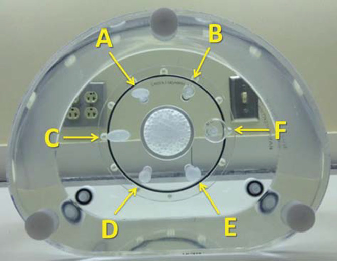
Modified NEMA IEC Body Phantom with spherical and ellipsoid inserts and corresponding naming scheme. [Color figure can be viewed at wileyonlinelibrary.com]

Table 1.

Shape, orientation, size, and volume of phantom inserts utilized

Insert	Shape and orientation	Diameter/Size (mm)	Volume (ml)
A	Ellipsoid, horizontal	20 × 10 × 10	1.0472
B	Sphere	13	1.1503
C	Ellipsoid, horizontal	26 × 13 × 13	2.3007
D	Ellipsoid, axial	26 × 13 × 13	2.3007
E	Ellipsoid, axial	34 × 17 × 17	5.1449
F	Sphere	28	11.4940

For the phantom experiments reported in this paper, a subset of 12 data sets was utilized by selecting two of the ten 3 minute scans for both high and low contrast for each of the two PET/CT scanners (one at UI and one at UW). In addition, each of the 30 minute scans for each of the scanners at both high and low contrast were selected. Table 2 provides a summary of scanner models and imaging parameters utilized for the subset.

Table 2.

Scanners and imaging parameters utilized for phantom PET scans

	UI	UW
Vendor	Siemens	GE Medical Systems
Scanner	Biograph 40	Discovery STE
Reconstruction	OSEM3D 4i8s	OSEM3D IR (4i28s)
Gaussian filter (mm)	7	3
Voxel size (mm)	3.394 × 3.394 × 2.025	2.734 × 2.734 × 3.270
Reconstruction matrix size	168 × 168	256 × 256
Number of slices	81	47

2.A.2. Clinical head and neck cancer PET scans

FDG PET/CT scans from patients with head and neck cancer (HNC) acquired at the University of Iowa Hospitals and Clinics were utilized for an assessment of segmentation performance on clinically relevant data sets. The data were collected, curated, and uploaded to TCIA (collection: QIN‐HEADNECK ${}^{20}$) as part of the NIH/NCI funded projects U01CA140206 and U24CA180918. For the experiments reported in this paper, a subset of baseline PET data sets were utilized, which were all pre‐treatment PET scans.

The imaging protocol for HNC data sets was as follows. Patients were fasted for a minimum of 6 hours, and the injected dose of ${}^{18}$F‐FDG was weight‐based with a maximum injected dose of 15 mCi. The uptake time was 90 ± 10 minutes between injection and start of image acquisition. Nine scans were acquired using a Siemens Biograph Duo and one with a Siemens Biograph 40 PET/CT scanner. For the Biograph Duo scanner, a 2D OSEM reconstruction algorithm with 2 iterations, 8 subsets, and a 5 mm Gaussian filter was used. The voxel size was 3.538 × 3.538 × 3.375 mm. The reconstruction matrix size was 128 × 128. For the Biograph 40 scanner, 2D OSEM reconstruction with 4 iterations, 8 subsets, and a 7 mm Gaussian filter was utilized. The voxel size was 3.394 × 3.394 × 2.025. The reconstruction matrix size was 168 × 168. The number of slices of the scans ranged between 191 and 545 (mean: 298.5). All PET scans were attenuation corrected using the corresponding CT scan.

All target structures to be segmented by participating QIN sites were pre‐identified by means of indicator images (Fig. 2), showing what lesion should be segmented and what label should be used for a lesion. All indicator images were generated by an experienced radiation oncologist (JMB) who inspected all scans, identified primary tumors and all positive (hot) lymph nodes considering the corresponding CT information as well as clinical patient records. To minimize the need for expert interpretation of HNC test cases, indicator images not only identify the lesion that should be segmented (Figs. 2(a) and 2(b)), but also show what neighboring structures should be avoided (red crosses in Fig. 2(c)). The complexity of defined segmentation tasks ranged substantially from patient to patient, and the number of lesions to be segmented per subject varied from 1 to 12 (mean: 4.7, median: 4). Overall, 47 lesions were required to be segmented in the ten PET scans.

Figure 2.

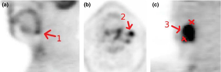
Example of indicator images. [Color figure can be viewed at wileyonlinelibrary.com]

2.B. Sites and segmentation approaches

The following seven QIN sites volunteered to segment the PET image data described in Sections 2.A.1. and 2.A.2: Columbia University Medical Center, H Lee Moffitt Cancer Center and University of South Florida, Memorial Sloan Kettering Cancer Center, Simon Fraser University (Canada), University of Pittsburgh, University of Iowa, and University of Washington Medical Center. Each site was allowed to use the segmentation tool of their own choice. Segmentation software included both commercially available software and academic, in‐house developed segmentation algorithms. An overview of the segmentation tools used in the challenge as well as the credentials of operators/users performing the semi‐automated segmentation at each site are given in Table 3. The approaches tested require varying degrees of user interaction for segmentation. Thus, users (skills) and algorithm combined create a segmentation approach. A detailed description of approaches one to seven is given below.

• Approach 1: In‐house developed software (“PETSegmentor”) implemented with C++ and Interactive Data Language (Harris Geospatial Solutions, Boulder, CO) was utilized for segmentation. The algorithm is based on an adaptive thresholding and a subsequent active contour segmentation step. First, two thresholds were derived from the SUV distribution inside a user specified region of interest (ROI). For this purpose, the user draws an elliptical ROI on one slice depicting the lesion. A volume of interest (VOI) was generated from the ROI. The VOI is a cuboid which has the width and length of the ROI in axial plane, and the height of the cuboid is 1.5 times the maximum of width and length. The cuboid is centered at the ROI plane. Second, one threshold $Thres{h}_{wa}$ is the geometric mean of $SU{V}_{max}$ and $SU{V}_{wa}$, where $SU{V}_{max}$ is the maximum SUV‐value in the region, and $SU{V}_{wa}$ is a weighted average of all the pixels inside the elliptical ROI. Pixels closer to the ROI boundary (background) have a high weight, and lesion pixels which are farther away from the boundary have a low weight. The weight is proportional to $exp(-d^2/(2s^2))$ where d is the distance to the ROI boundary and $s=d_{max}/3$. $d_{max}$ represents the maximum distance in the ROI to the boundary. The mean μ and standard deviation σ of the region inside the ROI and below the threshold were calculated. A second threshold $Thres{h}_{st}$ is set to μ + 3σ. The minimum of the two thresholds is taken as the threshold. Third, applying active contours directly on the image result in a contour that is a little too tight. So a gamma correction is applied with γ = 1/1.5 to compress the dynamic range of the lesion and expand the dynamic range of background, that is, $Valu{e}_{new}=Valu{e}_{max}{(Valu{e}_{old}/Valu{e}_{max})}^{\mathit{\gamma }}$. Finally, a local region based active contour method was applied to the enhanced volume.²²

• Approach 2: A semi‐automated segmentation method was utilized that transforms the segmentation problem into a graph‐based optimization problem.²¹ It was implemented as an extension for 3D Slicer, a multi‐platform, free, and open source software package for visualization and medical image computing.²³ To initiate segmentation, the user identifies roughly the center of a lesion. Then the algorithm calculates a segmentation based on local image characteristics. If needed, the resulting segmentation was interactively refined by utilizing computer‐aided, efficient segmentation refinement methods.

• Approach 3: For segmentation, Mirada Medical RTx 1.6.2 (Mirada Medical Ltd., Denver, CO) was used. First, a region of interest (ROI) was manually generated by utilizing sphere, ellipse, cube, or arbitrary region drawing tools. Second, segmentation was performed in 3D. For this purpose, uptake values were converted to standardized uptake values (SUVs) using body weight, and an automated segmentation procedure was started that used an absolute threshold of 2.5 SUV. Each voxel inside initial ROI with absolute value of SUV greater than or equal to 2.5 was marked as contoured. In the case where the maximum SUV value in a ROI is less than 2.5 SUV, a threshold of 42% of maximum intensity was used instead of the absolute threshold of 2.5 SUV. After automatic segmentation, the contoured ROI could be corrected by using several methods to fill holes in 2D/3D, remove disconnected regions, and smooth structures. The final contour did undergo slice‐by‐slice inspection in order to exclude false positive regions of high metabolic activity.

• Approach 4: A combination of the PET Volume Computer Assisted Reading (VCAR) v11.3‐10.11 tool implemented on the GE Advantage Workstation v4.6.05 (GE Healthcare, UK) and PMOD v3.504 (PMOD Technologies Ltd., Zurich, CH) was utilized. First, the adaptive thresholding algorithm of PET VCAR was utilized to find suitable segmentation thresholds on a lesion by lesion basis. To start the algorithm, the user identified the approximate center of a lesion. Second, due to encountered problems in saving the segmentation result, the calculated threshold values were transferred to PMOD and applied to the PET data. The resulting segmentations were saved using PMOD. Also, the user had the option to only select a single component of the thresholding result.

• Approach 5: Segmentation was performed by utilizing the PETedge tool of MIM v5.4.8 (MIM Software Inc., Cleveland, OH) software, which uses image gradient information for determining lesion boundaries.²⁴ For segmentation, the user roughly marked a region inside the lesion. This region was then utilized by the software to calculate the actual segmentation. If the produced segmentation was deemed unusable/incorrect, the initial start volume was reset and the segmentation method was rerun. In addition, MIM allowed the user to make minor manual edits to segmentations.

• Approach 6: Segmentation was performed by utilizing the automatic isocontour detection algorithm in the PMOD software package v3.506 (PMOD Technologies Ltd., Zurich, CH). All segmentations were based on an adjustable fraction (threshold) of the maximum pixel uptake value in the selected 3D VOI. First, the user was required to construct a 3D volume of interest (VOI) including the lesion to be segmented. Second, the user adjusted the threshold interactively to achieve the desired segmentation result. Note that for segmenting the phantom PET scans, an appropriately sized 3D VOI (sphere) was placed on the phantom uptake image around each of the six areas of activity, followed by a similar segmentation procedure for each of the six objects in the phantom scan.

• Approach 7: In‐house‐developed software (LevelPET 1.0) based on an energy‐minimizing 3D level‐set segmentation approach implemented in MATLAB (MathWorks, Natick, MA) was used. For technical details on this class of approaches, the reader is referred to earlier similar works on this topic.^{25, 26, 27} In short, to segment a lesion, a zero level‐set surface is initialized using one or more points (seeds), and then the surface is deformed to match the lesions in the 3D PET image. In particular, the deformation updates are a result of an optimization process that ensures the resulting segmentation surface (i) forms a smooth lesion boundary (by penalizing large surface areas); (ii) passes through voxels of high image intensity gradient magnitude;²⁷ and (iii) whose interior and exterior regions (inside and outside the surface) follow learned intensity priors. These three criteria are encoded as energy terms in an energy function. The intensity priors are Gaussian distributions whose mean and variance are estimated from sample pixels inside and outside the lesions.²⁶ For initialization of the lesion surface and for collecting the intensity priors, the user selected a single seed in the interior of a lesion in a 2D slice and selected one or more regions outside the lesion to collect intensity priors. Five scalar parameters needed to be set by the user to control the behavior of the level set: One parameter controls the influence of the smoothness term and four parameters (two pairs of starting and ending values) dictate how the influence of the gradient and intensity priors changes over iterations. A trial and error approach was utilized to adjust the parameters such that the method performs well for the majority of data sets to be segmented. The parameters for the method were fixed across all data sets with the exception for two out of 47 lesions. Also, for the cases where a specific lesion in close proximity should not be included in the segmentation, contours for the touching lesions were initialized separately.

Table 3.

Overview of utilized PET image segmentation approaches and credentials of operators performing the semi‐automated segmentation. See text in Section 2.B for details

Approach	Segmentation approach/software	Credentials of operators performing the semi‐automated segmentation
1	In‐house developed software based on an active contour segmentation approach	PhD research scientist
2	In‐house developed software utilizing a graph‐based optimization approach${}^{21}$	Radiation oncologist
3	Commercial software package	Imaging physicist
	Mirada Medical RTx
4	Combination of commercial software packages VCAR and PMOD	Medical physics postdoc
5	Commercial software package MIM	Imaging physicist
6	Commercial software package PMOD	Image Analyst
7	In‐house developed software based on 3D level‐set segmentation approach	Medical image analysis graduate student (familiar with 3D PET and image segmentation)

2.C. Experimental setup

All participants were required to segment both the phantom and HNC PET data described in Sections 2.A.1 and 2.A.2, respectively. Note that if a segmentation method failed to produce an accurate segmentation, the incorrect result was submitted and the event was reported. Similarly, if a lesion could not be segmented, it was also reported without submitting a segmentation. In addition, the time required for segmentation was recorded. Details regarding this procedure are given below. In addition, repeat segmentations were performed on both phantom and HNC PET data at a separate time to assess intrainstitutional consistency.

1. Phantom segmentation procedure: After downloading all 12 PET phantom data sets described in Section 2.A.1 from TCIA, the participating QIN sites were required to segment all six inserts in the scans with the segmentation approach of their choice (Section 2.B). After the initial segmentation, sites were required to wait at least one day before repeating the segmentation process for all 30 minutes scans and a given subset of four low statistics scans (i.e., one high and low contrast scan for each scanner).

2. HNC segmentation procedure: After downloading the ten HNC PET scans and corresponding indicator images, participants were required to segment all 47 lesions in the ten data sets. Following at least a one week waiting period, the segmentation process was repeated. Note that because HNC shapes are more complex than generic geometric primitives utilized as phantom inserts, a longer waiting period was used to avoid operators remembering the shapes of previously segmented lesions.

All segmentations were required to be stored in DICOM RT or DICOM SEG data format. After segmentation, results were uploaded to NCIP Hub,${}^{28}$ a collaborative space for NCI‐related informatics in cancer research. Subsequently, a quantitative volume‐based analysis was performed. For this purpose, the volume was derived from all segmentations and compared to an independent reference standard. For phantom data, the volume of the inserts served as a ground truth (Table 1). In the case of HNC image data, three experienced radiation oncologists manually segmented all lesions identified by the generated indicator images (Section 2.A.2). The manual segmentation was performed twice on different days by all three radiation oncologists. The resulting volumes were averaged in order to reduce inter‐ and intra‐reader variability in the HNC reference standard. Statistical analysis was performed on the derived volumes as described in Section 2.D.

2.D. Statistical analysis

Measured phantom and HNC tumor volumes (v) were summarized and compared to the reference volumes with descriptive statistics and plots. Summaries include measured versus reference volume, relative error, relative mean error, and relative repeat error. The relative error is defined as

$$\text{Relative}{\text{Error}}_{i,j,k}=\frac{v_{i,j,k}-v_{\mathrm{ref},j}}{v_{\mathrm{ref},j}}100\%,$$

where $v_{i,j,k}$ is the $k^{\mathrm{th}}$ volume measurement from approach i and insert/tumor j, and $v_{\mathrm{ref},j}$ is the corresponding reference volume. Differences in average measured volumes are reported as relative mean error, defined as

$$\text{Relative Mean}{\text{Error}}_{i,j}=\frac{{\overline{v}}_{i,j}-v_{\mathrm{ref},j}}{v_{\mathrm{ref},j}}100\%,$$

where ${\overline{v}}_{i,j}$ is the average measured volume for insert/lesion j and approach i. Averages were computed separately for each insert in the phantom data and were estimated with locally weighted scatterplot smoothing (LOESS) across the continuous range of tumor volumes in the HNC data. Relative mean error represents approach‐specific biases that exist in measured tumor volumes. To summarize errors in volumes from repeated segmentation, the relative repeat difference was calculated as the difference between repeats divided by the corresponding reference volume. Relative error and repeat differences are summarized with means and standard deviations to quantify bias and variability, respectively. Additionally, the root mean squared (RMS) error/difference was computed as the square root of the mean of squared relative errors/differences and is reported as a composite measure of bias and variability.

Effects of approaches, scanners, scanner conditions (statistics and contrasts), repeated segmentation, and repeated scans on the variability in measured volumes were estimated with linear mixed effects regression models. The fitted phantom model was of the form

$$\begin{array}{cc}\hfill logv=& {\mathit{\beta }}_{\mathrm{insert}}+{\mathit{\gamma }}_{\mathrm{scanner}}+{\mathit{\gamma }}_{\mathrm{insert}\ast \mathrm{scanner}}+{\mathit{\gamma }}_{\mathrm{approach}}\hfill \\ & +{\mathit{\gamma }}_{\mathrm{approach}\ast \mathrm{insert}\ast \mathrm{scanner}}+{\mathit{\gamma }}_{\mathrm{contrast}}+{\mathit{\gamma }}_{\mathrm{statistic}}\hfill \\ & +{\mathit{\gamma }}_{\mathrm{scan}}+{\mathit{\epsilon }}_{\mathrm{segmentation}},\hfill \end{array}$$

where β was a fixed effect; γ and ɛ were normally distributed random effects and residual error terms, respectively; and effects were included for interactions between inserts and scanners (insert*scanner) as well as approach (approach*insert*scanner). A log‐linear relationship between measured volumes and sources of variability was specified for the analysis in order to normalize the residuals and stabilize their variance.

HNC volume, measured across a range of tumor sizes, was modeled as the following function of reference volumes (x) from the experienced radiation oncologists:

$$logv=\mathit{\beta }logx+{\mathit{\gamma }}_{\mathrm{approach}}+{\mathit{\gamma }}_{\mathrm{lesion}*\mathrm{patient}}+{\mathit{\gamma }}_{\mathrm{approach}*\mathrm{lesion}*\mathrm{patient}}+{\mathit{\epsilon }}_{\mathrm{segmentation}}.$$

As with phantom scans, scan source, contrast, and statistic conditions can affect volume measurements from HNC scans. Such effects are adjusted for with the inclusion of expert reader volumes in the regression model. In particular, scan condition effects are reflected in volumes measured by the expert reader since they were made on the same set of scans reviewed by the approach‐specific operators. As a diagnostic check, contrast was explicitly quantified and evaluated in the regression model, found to be non‐significant statistically, and thus left out in the final analysis. Since scan conditions were adjusted for in both the phantom and HNC models, resulting estimates of approach and repeated segmentation variability could be compared directly between the two settings.

From the fitted (final) regression models, relative mean error was computed as the difference between estimated mean and reference volumes, divided by the reference; standard deviation estimates were obtained for each of the random effects and residual errors; and percent coefficient of variation (CV) was calculated as 100% times the standard deviations divided by the means. As estimated from the regression models, the CV is constant with respect to insert/lesion volume. The CV estimates are reported along with 95% confidence intervals and compared using Wald test statistics. All statistical testing was 2‐sided and assessed for significance at the 5% level. Analyses were performed with the SAS version 9.4 (Cary, NC) and R statistical software (R Core Team).

3. Results

Results of our study will be presented in three parts. First, results grouped by insert/lesion volume will be presented (Section 3.A). Second, results grouped by segmentation approach will be summarized (Section 3.B). Third, regression analysis results enabling the direct comparison of results on phantom and HNC scans will be given (Section 3.C).

3.A. Results grouped by insert/lesion volume

The relative mean error for each of the six phantom inserts is summarized in Table 4. Insert‐specific summary statistics are aggregated over segmentation approaches, scanners, scan conditions, repeated segmentations, and repeated scans. Figures 3(a) and 3(b) provide boxplots for each insert per scanner, and Fig. 3(c) provides a summary over both scanners per insert. Overall, segmentation derived volumes are larger than the known insert volumes. With smaller insert volume, increases in relative error mean and standard deviation are noticeable.

Table 4.

Summary of volume measurements for phantom scans by insert

Insert	Measurements (N)	Reference volume (ml)	Relative error (%)
			Mean	SD	RMS
A	133	1.05	77.7	136.0	156.2
B	133	1.15	67.0	101.5	121.3
C	135	2.30	52.8	81.1	96.5
D	133	2.30	43.1	71.3	83.1
E	136	5.14	29.4	52.4	59.9
F	136	11.49	23.6	40.6	46.8

Figure 3.

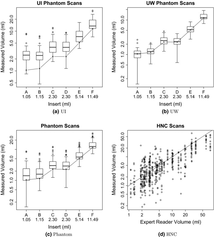
Distributions of measured volumes by reference volumes. The gray diamonds (phantom) and line (HNC) represent the reference volumes. Note that phantom and HNC plots have different scales.

The results of a more detailed analysis that takes image statistics, contrast ratios, and utilized scanner into account are summarized in Table 5. Boxplots for both PET scanners are given in Figs. 3(a) and 3(b). As can be seen from the table as well as the figures, segmentations of the UI phantom scans, reconstructed with a larger Gaussian smoothing filter (7 mm), show a clear bias towards over segmentation leading to larger volume measurements. In contrast, the segmentations based on the UW phantom scans, reconstructed with a narrower Gaussian smoothing fiter (3 mm), show little or no over segmentation bias, resulting in a lower overall error (Table 5). Also, as Table V(a) shows, the volume bias increases with decreasing insert volume on segmentations of UI phantom scans. Furthermore, on UI and UW phantom data, one can notice that phantom scans with higher contrast result in a higher average relative error.

Table 5.

Mean relative errors (%) in measured volumes for phantom scan measurements by acquisition condition and insert. (a) UI phantom PET scans. (b) UW phantom PET scans

Condition		Insert						Overall
Statistics	Contrast	A	B	C	D	E	F
(a)
LO	LO	144.4	99.2	89.4	63.9	38.8	22.3	76.3
LO	HI	276.1	214.6	144.2	132.7	86.8	63.9	153.1
HI	LO	87.6	79.4	38.8	49.1	23.9	20.3	49.9
HI	HI	82.3	79.5	66.2	78.0	50.5	42.5	66.5
Overall		147.6	118.2	84.6	80.9	50.0	37.2	86.4
(b)
LO	LO	5.2	2.4	−3.1	−13.3	−7.2	−0.7	−2.8
LO	HI	7.7	24.1	33.7	18.7	15.7	18.1	19.7
HI	LO	−26.1	−12.6	−1.3	−9.0	−2.2	1.8	−8.3
HI	HI	−0.3	24.1	30.2	20.0	22.8	17.7	19.1
Overall		−3.4	9.5	14.9	4.1	7.3	9.2	6.9

Table 6 summarizes the relative mean error for HNC segmentations, using volume bins that roughly match the volumes of the phantom inserts and have approximately the same cardinality. These HNC summary statistics are aggregated over segmentation approaches and repeated segmentations. The scatter plot given in Fig. 3(d) enables a comparison between expert reader defined reference volume and the volume generated by the investigated segmentation approaches. As Table 6 shows, the volume bias trends from over estimation to underestimation with increasing lesion volume, while the standard deviation steadily decreases.

Table 6.

Summary of volume measurements for HNC scans by reference tumor volumes

Reference interval (ml)	Measurements (N)	Relative error (%)
		Mean	SD	RMS
0–2.25	106	34.5	151.5	154.7
2.26–3.02	106	25.6	102.4	105.1
3.03–5.06	120	16.7	107.7	108.6
5.07–13.89	105	−9.2	53.1	53.7
13.90+	120	−39.2	33.3	51.3

3.B. Results grouped by segmentation approach

Tables VII(a) and VII(b) provide mean, standard deviation (SD), and RMS summaries of relative error, and Fig. 4 plots the relative mean error. Phantom summary statistics are aggregated over 6 inserts, 2 scanners, 4 scan conditions, 2 repeated segmentations, and 2 repeated scans. Repeated scans were only performed on 2 of the scan conditions and without repeated segmentation, for a maximum of 120 volume measurements per segmentation approach. HNC statistics are aggregated over 47 lesions and 2 repeated segmentations, for a maximum of 94 volume measurements per approach. Phantom volume measurements tended to be upwardly biased across all approaches. HNC measurements were upwardly biased for three approaches (1, 4 and 7), similar to phantom scans, and downwardly biased for the other approaches. Approach 4 was an extreme outlier with respect to relative HNC errors (mean = 701.5, SD = 1402.6) and was thus excluded from all subsequent HNC analyses. Boxplots of relative errors in Fig. 5 summarize the distributions of differences between measured and reference measurements by approach. Their medians represent overall approach‐specific bias. Spread in the distributions represents variability due to approaches, scanners (UI vs UW), scan conditions, repeated segmentations, and repeated scans for phantom scans and due to approach and repeated segmentation for HNC scans. The boxplots of the relative repeat error in Fig. 6 show variability due to repeated segmentation by approach, independent of other sources of variability.

Table 7.

Relative errors by approach for (a) phantom scans and (b) HNC scans

Approach	Measurements (N)	Relative error (%)			Repeat difference (%)
		Mean	SD	RMS	Mean	SD	RMS
(a)
1	120	70.5	87.5	112.0	5.9	24.8	25.2
2	120	58.1	55.3	80.0	0.1	5.3	5.3
3	120	33.8	58.4	67.2	−36.4	54.6	65.2
4	86	87.8	179.2	198.7	−0.1	7.2	7.1
5	120	41.3	48.9	63.8	4.4	19.1	19.4
6	120	31.0	83.8	89.1	39.9	57.7	69.7
7	120	29.9	58.0	65.0	−6.3	26.0	26.5
(b)
1	94	82.1	169.6	187.6	−37.7	196.5	198.0
2	94	−5.6	35.7	36.0	−1.5	30.4	30.1
3	91	−21.0	44.4	48.9	31.5	56.2	63.8
4	84	701.5	1402.6	1560.8	−0.6	332.4	328.5
5	94	−25.4	48.6	54.6	21.8	56.3	59.8
6	92	−50.5	26.0	56.8	2.1	26.8	26.6
7	92	48.6	119.4	128.3	6.5	37.7	37.8

Figure 4.

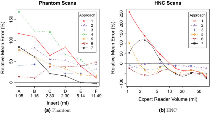
Approach‐specific relative mean error as a function of reference volume. [Color figure can be viewed at wileyonlinelibrary.com]

Figure 5.

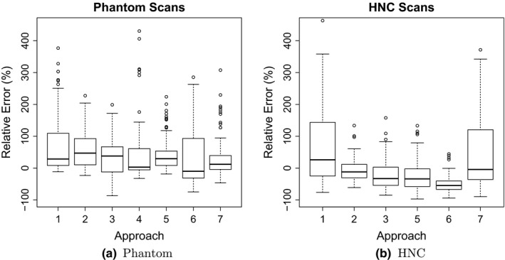
Distributions of relative errors in volume measurements by approach.

Figure 6.

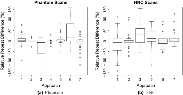
Distributions of relative repeat errors in volume measurements by approach.

Additional segmentation performance indices (Dice coefficient and unsigned distance error) on HNC data are provided in Appendix A.

In some cases, the utilized segmentation software failed to produce a segmentation result or was not able to load a particular set of PET scans (Approach 4). In such a case, no segmentation results were submitted for analysis. The absolute and relative number of failures (i.e., not submitted insert and lesion segmentations) was as follows. On phantom data, only approach 4 was not able to segment 34 (28.3%) inserts. On HNC data, approach 3 had 3 (3.2%), approach 4 had 10 (10.6%), and approaches 6 and 7 had each 2 (2.1%) failures. In addition, approach 1 produced clearly erroneous results in nine cases (9.6%), which were submitted for analysis. Also, approach 7 required different parameters for two lesions so that the approach was able to produce an acceptable segmentation result.

The required segmentation time per data set was as follows. On phantom data, all approaches required low (t ≤ 5 min) user effort. On HNC data, approaches 1, 2, and 7 required low, approach 5 required medium (5 min  < t ≤ 10 min), approaches 3, 4, and 6 required high (10 min  < t ≤ 20 min) effort. Note that for approach 7, the reported segmentation time did not include trial and error based manual optimization of segmentation parameters.

Examples for segmentation results on HNC PET images and an example of corresponding manual reference segmentation as well as quantitative segmentation performance indices are given in Figs. 7 and 8.

Figure 7.

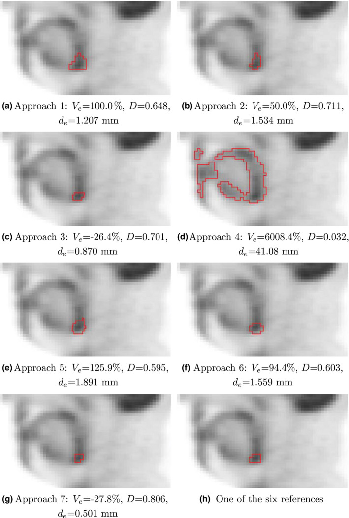
Examples of segmentation results for a primary cancer site, which is part of test set HNC. (a–g) Segmentations generated with approaches 1 to 7. (h) One example of the six manual reference segmentations. The corresponding indicator image is given in Fig. 2(a). For each segmentation approach, the relative volume error $V_e$, Dice coefficient D, and mean unsigned distance error $d_e$ is provided. [Color figure can be viewed at wileyonlinelibrary.com]

Figure 8.

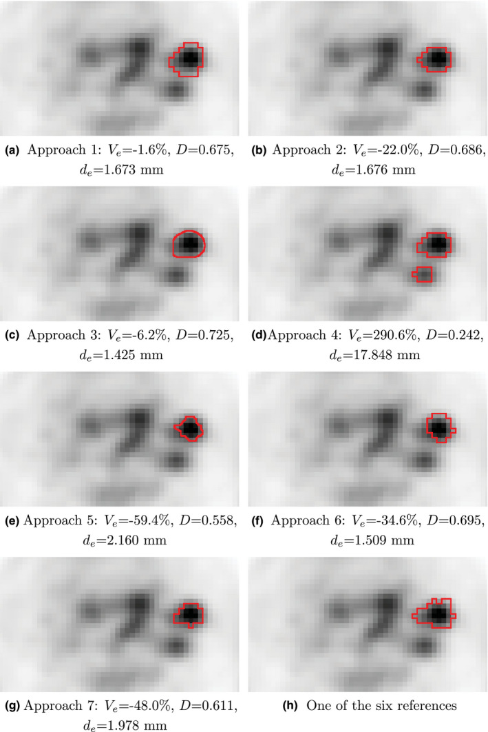
Examples of segmentation results for a hot lymph node, which is part of test set HNC. (a–g) Segmentations generated with approaches 1 to 7. (h) One example of the six manual reference segmentations. The corresponding indicator image is given in Fig. 2(b). For each segmentation approach, the relative volume error $V_e$, Dice coefficient D, and mean unsigned distance error $d_e$ is provided. [Color figure can be viewed at wileyonlinelibrary.com]

3.C. Results of regression analysis

Regression analysis was performed to estimate relative mean error and variance components for the combination of all participant sites. Modeled relative mean errors over all measurements are shown in Figs. 9(a) and 9(b) for phantom and HNC segmentation data, respectively. For Fig. 9(a), the relative means for UI and UW phantom scans are depicted in addition to the overall mean, which represent the largest source of variation in the phantom data. Statistical comparisons of the overall relative mean errors between phantom and HNC scans were not found to be significantly different.

Figure 9.

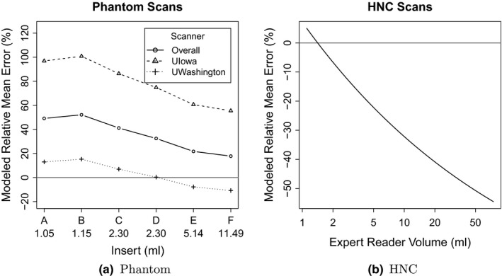
Relative mean errors from regression modeling of the phantom and HNC data.

The phantom study design allowed variability components to be estimated separately for approaches, scanners (UI vs. UW), statistics (high vs. low), contrasts (high vs. low), repeated scans (1 vs. 2), and repeated segmentations (1 vs. 2). Components for the HNC scans are reported for approaches and repeated segmentations, with variability due to the other components (scanners, statistics, and contrasts) adjusted for with the inclusion of expert reader volumes in the model. Coefficient of variation (CV) estimates are shown in Table 8 for the different variability components included in the regression models. The CV for approaches was significantly different from statistics within phantom scans (26.8% vs. 5.3%, P = 0.0307). Comparisons of other CV estimates within phantom scans and within HNC scans were not significantly different. In comparisons between phantom and HNC scans, CV estimates were approximately twice as large for HNC scans. In particular, the CVs for different approaches were 57.0% for HNC and 26.8% for phantoms (P = 0.0240); whereas, repeated segmentation CVs were 42.7% and 21.1% (P < 0.0001), respectively.

Table 8.

Modeled percent coefficient of variation estimates and 95% confidence intervals for variability components

Variability component	Coefficient of variation (95% CI)		P‐value
	Phantom scans	HNC scans
Scanners (UI, UW)	42.5 (9.0–201.1)	NA	NA
Approaches	26.8 (20.5–35.1)	57.0 (35.3–92.0)	0.0240
Repeated segmentations	21.1 (19.9–22.3)	42.7 (38.2–47.8)	<0.0001
Contrasts	14.3 (3.3–61.2)	NA	NA
Statistics (acquisition time)	5.3 (1.2–22.4)	NA	NA
Repeated scans	0.0	NA	NA

4. Discussion

To implement consistent quantitative imaging metrics and thereby radiomics, a robust processing pipeline that includes components like image acquisition, target object segmentation, feature generation, and analysis is needed. Clearly, any processing chain can only be as strong as its weakest link. The goal of this study was to assess bias and variability of 3D segmentation performance measured by segmentation volume analysis of both phantom image data sets with known volumes acquired under a variety of different conditions (scanner, statistics, and contrast variations) and consistently acquired human oncology PET imaging data for analysis using a variety of segmentation approaches across institutions on a national level by utilizing the QIN network. These sources of variability will need to be minimized to optimally harness the potential of quantitative imaging for clinical trial support and ultimately clinical decision making in oncology.

4.A. Performance on phantom and HNC PET data

Based on the phantom and HNC analysis results presented in Section 3, we draw the following conclusions.

• Bias: A large bias in segmentation volumes was measured. This bias was found to depend on the phantom insert/clinical lesion size, and therefore cannot be assumed to be constant (Fig. 9). The size‐dependent variation/change of bias was found to be larger for clinical HNC data compared to phantom data, although the difference was not statistically significant.

• Variation: Results presented in Table 8 indicate that considerable variability was introduced by utilizing different segmentation approaches and performing repeated segmentations using the same approach. Given the measured CV levels, it seems very likely that such variations will adversely impact the stability of segmentation‐derived features, and ultimately, classification performance of a radiomics system. These variations can be seen as measurement “noise” that make it more difficult to train a classifier or to clearly distinguish between desired class labels. Many papers use phantoms for method evaluation, optimization, and performance assessment, because of the known ground truth. While phantom studies have an important role, our study clearly demonstrates the limits of phantom analyses. Volume determination by different institutions and repeated determination within the same institution had variability and this was estimated with regression analysis, independent of scan conditions, and therefore can be compared directly between phantom and HNC scans. The variability introduced by utilizing different segmentation approaches was found to be significantly larger ( + 112.7%) for segmentations of clinical HNC PET images compared to phantom data. Similarly, the volume variation due to repeated segmentation was also found to be significantly larger ( + 102.4%) for segmentations of the clinical HNC data compared to phantom data.

• Time: While the time required for PET phantom segmentation for all seven approaches was low, results on clinical HNC data were less homogeneous, spreading from low to high time complexity (Section 3.B). However, three approaches managed to keep segmentation time low.

• Failure: Two approaches managed to tackle all segmentation tasks without any failures or major errors (Section 3.B). Across methods, more failures were reported on the clinical HNC test sets compared to phantom test sets, suggesting higher complexity of HNC PET scans. In addition to the conclusions presented above, the phantom‐based experiments resulted in the following observations.

• Imaging equipment and reconstruction: The imaging setup (PET scanner model, reconstruction parameters, etc.) is responsible for the largest CV component with a value of 42.5%, and the impact on volume bias is clearly visible in Fig. 9(a). A major difference between the two imaging setups tested (UI and UW)—besides the different scanner models— was the degree of Gaussian smoothing utilized (Table 2), which is representative of lower and upper limits of typically utilized kernel sizes. This clearly demonstrates the essential need for harmonization of image reconstruction approaches for quantitative analyses in clinical trials. Quantitative harmonization efforts, supported by all major PET/CT manufacturers, are currently being pursued through NCI funded academic‐industrial initiatives (R01 CA169072) and coordinated through the Society of Nuclear Medicine and Molecular Imaging and the European Association of Nuclear Medicine.

• Contrast vs. statistics: Although not found to be statistically significant, increasing contrast led to a higher CV compared to count statistics (acquisition time). This “pattern” is also noticeable across different insert sizes (Table 5).

• Repeated scans: Variability introduced by performing repeated PET scans of the phantom was not measurable statistically, when accounting for the other variability components, suggesting that the stochastic component in PET images induced by repeated scans can be neglected for the scanners investigated.

4.B. Performance comparison between approaches

The segmentation methods investigated in this study cover a broad spectrum, ranging from those that are commercially available, application nonspecific software to custom‐build in‐house segmentation algorithms. All methods investigated required input from a user to produce meaningful segmentations. This is especially true for clinically relevant HNC PET scans with a complex array of pathology (cancer) and other anatomical structures with uptake. Consequently, it is not possible to differentiate between method intrinsic and operator performance. While it is desirable that semi‐automated segmentation tools are operated by physicians, this may be difficult due to cost and time constraints in some circumstances (i.e., a large clinical trial analysis). In such cases it may be more realistic that manual interaction requirements be performed by trained personnel with oversight by a physician expert. In our study we tried to simulate this scenario by providing detailed radiation oncologist generated indicator images (Fig. 2) to guide the user and eliminate the need for access to patient records. In this context, we recognize that performing lesion segmentation for quantification of treatment response is currently not standard practice, and radiomics approaches—while promising—are currently in a research or development stage. Hence, some sites may be more proficient at generating 3D lesion segmentations in PET images than others. Also, there is no explicitly dedicated personnel available in clinics for such tasks, which falls somewhere between the competences of Radiology, Oncology, and Radiation Oncology departments. Because of this, limiting the need for skilled and potentially discipline specific operator performance is desirable.

Differences between performance of segmentation approaches are quite large (Table 7, Figs. 5 and 6). Figs. 10(a) and 10(b) summarize root mean squared (RMS) values for relative repeat error and repeat difference for phantom and HNC data, respectively. A flawless method (i.e., zero relative error and zero repeat difference) would result in a point at the coordinate system origin at (0,0). Approaches with corresponding points closer to the origin are preferable. Overall approach performance is given by the plot in Fig. 11, which combines results from phantom and HNC studies to derive the RMS of phantom and HNC RMS values ($RM{S}_{all}$). As can be seen from Figs. 10 and 11, a number of methods show similar relative RMS error values, but differ considerably in terms of repeatability, which was assessed with the RMS repeat difference. In addition, there is performance variation within a given approach in terms of dependence on insert/lesion size, contrast, etc. (Fig. 4). For example, while approach 6 shows a relative constant bias across lesion size on HNC data, the relative mean error of approaches 1 and 7 changes from over‐segmentation to under‐segmentation (Fig. 4(b)). Also, as the plots given in Figs. 10 and 11 as well as the examples depicted in Figs. 7 and 8 demonstrate, an approach utilized by one site may not be sufficient for more complex PET image segmentation tasks.

Figure 10.

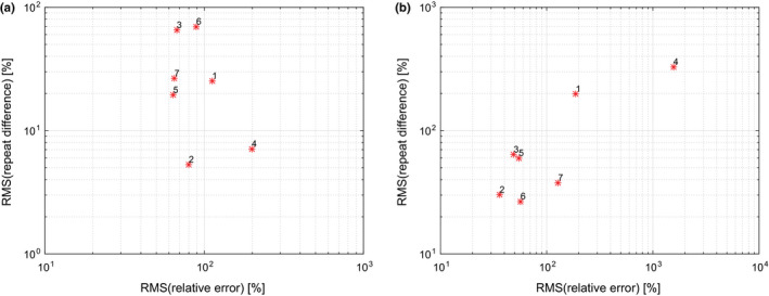
Comparison of segmentation performance of methods 1 to 7 on (a) phantom and (b) HNC data. [Color figure can be viewed at wileyonlinelibrary.com]

Figure 11.

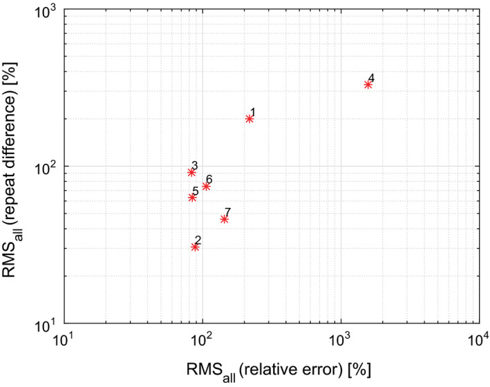
Overview of overall segmentation performance, comparing Methods 1 to 7. [Color figure can be viewed at wileyonlinelibrary.com]

4.C. Implications

Radiomics benefits from automated, high throughput processing that can improve consistency as well as efficiency in reducing the time needed to interact with the images to generate volumes for quantitative metric/feature generation. While method development in medical image analysis is progressing rapidly, the ultimate goal of fully automated, robust segmentation and quantification of lesions in clinical FDG PET images has not been reached yet. Therefore, to advance quantitative image based radiomics research, semi‐automated methods can be effectively used. These can reduce variability and speed tasks essential for analysis significantly. This study provides an assessment of potential pitfalls in multi‐site segmentation performance and should be considered in the context of clinical trials. Our study suggests the essential need for both harmonization of image reconstruction and acquisition parameters as well as the importance of improving analysis methods with robust and consistently applied semi‐automated tools. Results indicate site specific differences in segmentation and repeat performance. Note that the goal of this study was not to find the limit of harmonization. Instead, the intention was to quantify the current status. There are many avenues to harmonize and improve multi‐site FDG PET segmentation performance, including advancement and standardization of segmentation methods as well as analysis guidelines and user training. Also, application specific method development could be helpful. In addition, realistic widely available FDG PET segmentation benchmark data sets that consist of phantom and clinically relevant PET volumes are needed to advance algorithm development and enable objective comparison of method performance.

Development of consistently applied tools along with image acquisition and reconstruction harmonization will significantly improve the utility of quantitative imaging metrics for response assessment in clinical trials and the discipline of radiomics more generally. The potential of well designed tools that have minimized the requirements for user operability will also be important. In our current state, centralization of analysis, using a defined method appears essential, however, this does not suggest that this is an optimal approach for future practical clinical decision making. In the future, tools may be incorporated into scanner system software versus a software platform for analysis that provides user friendly and reliable data for decision making. Such tools would enable de‐centralization and clinical applicability if validated appropriately.

The majority of inserts and lesions utilized in this study are rather small, especially when compared to PET image voxel size. Therefore, partial volume effects need to be considered, which can influence segmentation performance. PET images with higher resolution will likely reduce such effects, but might also reveal inhomogeneity of tracer uptake in lesions, which could in turn impact performance. Thus, further studies are required, once PET scanners with increased spatial resolution become available for use in clinical trials and daily clinical routine.

4.D. Limitations and future work

The utilized PET phantom had inserts with a wall thickness of approximately 0.9 mm. As demonstrated by the work of Hofheiz et al.²⁹ and Berthon et al.,³⁰ such cold walls in combination with active background represent a potential challenge for segmentation methods and can lead to a segmentation bias. Thus, results reported on the phantom (Section 3) should be interpreted as an upper bound. Consequently, the true performance differences between phantom and clinical HNC data might be even more pronounced. Future work will focus on comparisons based on phantoms that are not prone to cold wall effects, similarly as described elsewhere.^{31, 32} In this context, more complex phantoms and PET simulation tools (for examples see33, 34) are gaining popularity and promise to enable a more realistic assessment of PET segmentation performance compared to simpler phantoms like the one used in our study.

Due to a lack of ground truth for HNC FDG PET data, the study used reference segmentations that were manually generated by three expert readers. Naturally, the choice of a reference has the potential to affect estimates of bias and variability. For instance, bias estimates will be shifted downward if a reference standard would consist of systematically larger segmentations, and shifted upwards if they would be systematically smaller. The reported mean summaries of relative error and root mean squared error reflect bias and are thus affected by any systematic tendencies of the expert readers in segmenting lesions, although HNC bias was not found to be statistically different from phantom bias. In addition to bias, manually generated reference segmentations are subject to inter‐ and intra‐reader variability and can thus introduce and inflate estimates of study‐specific variability components (approach and repeated segmentation). Thus, to minimize such effects, lesions were segmented twice by three readers and the resulting volumes averaged together to produce the references used in this study. As an additional benefit of the repeated manual segmentations obtained, we were able to estimate inter‐ and intra‐reader variability to be 1% and 5% of the total variability in resulting volumes, respectively. The relatively small amounts of variability due to readers coupled with our averaging of their volumes suggest that the references used are unlikely to have a substantial effect on reported estimates of bias and variability.

The volume of segmentations was chosen as the main segmentation performance metric for the following reasons. First, it fully reflects the volumetric nature of the problem, which is in contrast to the 1D length measurement in RECIST.³⁵ Second, in the case of phantom data sets, the ground truth volume is readily available. In contrast, utilizing the DICE coefficient for phantom data would require a segmentation (e.g., PET or CT scan of phantom), which would likely introduce a bias and/or source of variability, and therefore, defeats the main purpose of using a phantom.

Once an insert/lesion segmentation is available, a number of different features can be calculated. Some features might be more stable despite varying segmentation volumes than others. In the future, the authors plan on studying this issue in more detail to rank typically utilized features regarding their robustness—and ultimately—assess the impact on radiomics systems. While features that are less volume dependent may currently be more stable they may limit the potential of more robust radiomics analyses if improved processes and methods are not developed.

5. Conclusion

For utilizing radiomics in oncology applications, it is imperative to produce accurate and repeatable segmentations of PET images to facilitate generating suitable image‐derived features. The presented work demonstrates the current challenges in multi‐site object segmentation in FDG PET volumes. Results highlight the importance of imaging and segmentation approach harmonization. Clearly, to be successful, this requires an interdisciplinary national/international effort. NCI's QIN represents an important step in this direction. In addition, future research in the area of fully or highly automated segmentation algorithms will help facilitating radiomics research, and ultimately, utilization of radiomics in a routine clinical setting.

Conflict of Interest Disclosure

The authors have no conflict of interest to report.

Appendix A.

Additional segmentation performance indices on HNC data

Because the independent reference standard used for HNC PET image segmentation assessment is available in the form of labeled volumes (i.e., masks for each lesion), additional segmentation performance indices can be calculated. Table 9 provides values and repeat differences of Dice coefficients and mean unsigned distance errors per approach. The scatter plots depicted in Figs. 12(a) and 12(b) compare the absolute values of the mean relative volume error per approach that are listed in Table VII(b) against the mean Dice coefficient and the mean unsigned distance error, respectively. The high degree of correlation between volume error and each of the other two indices suggests that performance comparisons based on the latter would produce conclusions similar to those reported in the main text. Corresponding boxplots of the additional performance indices can be found in Fig. 13.

Figure 12.

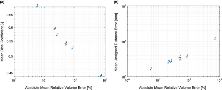
Comparison of the absolute mean relative volume error of approaches 1 to 7 against the corresponding mean Dice coefficient (a) and mean unsigned distance error (b). [Color figure can be viewed at wileyonlinelibrary.com]

Figure 13.

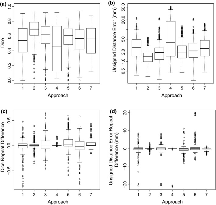
Boxplots of measured Dice coefficients (a) and unsigned distance errors (b) as well as corresponding repeat differences (c and d).

Table 9.

Dice coefficient and distance based segmentation performance indices on HNC data per segmentation approach

Approach	Measurements (N)	Dice coefficient				Unsigned distance error
		Values (‐)		Repeat differences (‐)		Values (nm)		Repeat differences (nm)
		Mean	SD	Mean	SD	Mean	SD	Mean	SD
1	94	0.524	0.199	−0.020	0.148	3.57	2.66	−0.10	2.73
2	94	0.683	0.126	0.006	0.045	1.58	0.67	−0.05	0.32
3	91	0.593	0.186	0.013	0.159	2.46	2.49	−0.27	3.34
4	84	0.439	0.300	0.005	0.025	11.43	14.18	−0.50	3.17
5	94	0.570	0.155	0.070	0.153	2.58	1.84	−0.47	2.06
6	92	0.537	0.186	−0.019	0.164	2.96	2.60	0.61	3.30
7	92	0.542	0.178	0.039	0.072	3.49	2.69	−0.38	0.70

References

- 1. Cook GJR, Siddique M, Taylor BP, et al. Radiomics in PET: principles and applications. Clinical and Translational Imaging. 2014;2:269–276. [Google Scholar]
- 2. Kumar V, Gu Y, Basu S, et al. Radiomics: the process and the challenges. Magn Reson Imaging. 2012;30:1234–1248. [DOI] [PMC free article] [PubMed] [Google Scholar]
- 3. Alluri KC, Tahari AK, Wahl RL, et al. Prognostic value of FDG PET metabolic tumor volume in human papillomavirus‐positive stage III and IV oropharyngeal squamous cell carcinoma. AJR Am J Roentgenol 2014;203:897–903. [DOI] [PMC free article] [PubMed] [Google Scholar]
- 4. Sridhar P, Mercier G, Tan J, et al. FDG PET metabolic tumor volume segmentation and pathologic volume of primary human solid tumors. AJR Am J Roentgenol 2014;202(5):1114–1119. [DOI] [PubMed] [Google Scholar]
- 5. Dibble EH, Alvarez AC, Truong MT, et al. 18F‐FDG metabolic tumor volume and total glycolytic activity of oral cavity and oropharyngeal squamous cell cancer: adding value to clinical staging. J Nucl Med. 2012;53:709–715. [DOI] [PubMed] [Google Scholar]
- 6. Boellaard R, Delgado‐Bolton R, Oyen WJ, et al. FDG PET/CT: EANM procedure guidelines for tumour imaging: version 2.0. Eur J Nucl Med Mol Imaging 2015;42:328–354. [DOI] [PMC free article] [PubMed] [Google Scholar]
- 7. Graham MM, Wahl RL, Hoffman JM, et al. Summary of the UPICT Protocol for 18F‐FDG PET/CT Imaging in Oncology Clinical Trials. J Nucl Med 2015;56:955–961. [DOI] [PMC free article] [PubMed] [Google Scholar]
- 8. Delbeke D, Coleman RE, Guiberteau MJ, et al. Procedure guideline for tumor imaging with 18F‐FDG PET/CT 1.0. J Nucl Med 2006;47:885–895. [PubMed] [Google Scholar]
- 9. Quak E, Le Roux PY, Hofman MS, et al. Harmonizing FDG PET quantification while maintaining optimal lesion detection: prospective multicentre validation in 517 oncology patients. Eur J Nucl Med Mol Imaging 2015;42:2072–2082. [DOI] [PMC free article] [PubMed] [Google Scholar]
- 10. Lasnon C, Desmonts C, Quak E, et al. Harmonizing SUVs in multicentre trials when using different generation PET systems: prospective validation in non‐small cell lung cancer patients. Eur J Nucl Med Mol Imaging. 2013;40:985–996. [DOI] [PMC free article] [PubMed] [Google Scholar]
- 11. Kelly MD, Declerck JM. SUVref: reducing reconstruction‐dependent variation in PET SUV. EJNMMI Res. 2011;1:16. [DOI] [PMC free article] [PubMed] [Google Scholar]
- 12. Sunderland JJ, Christian PE. Quantitative PET/CT scanner performance characterization based upon the society of nuclear medicine and molecular imaging clinical trials network oncology clinical simulator phantom. J Nucl Med 2015;56:145–152. [DOI] [PubMed] [Google Scholar]
- 13. European Association of Nuclear Medicine EARL FDG‐PET/CT accreditation. http://earl.eanm.org/cms/website.php?id=/en/projects/fdg_pet_ct_accreditation.htm (2015) Accessed 12 January 2015.
- 14. Foster B, Bagci U, Mansoor A, et al. A review on segmentation of positron emission tomography images. Comput Biol Med. 2014;50:76–96. [DOI] [PMC free article] [PubMed] [Google Scholar]
- 15. Shepherd T, Teras M, Beichel RR, et al. Comparative study with new accuracy metrics for target volume contouring in PET image guided radiation therapy. IEEE Trans Med Imaging. 2012;31:2006–2024. [DOI] [PMC free article] [PubMed] [Google Scholar]
- 16. Hatt M, Cheze Le Rest C, Albarghach N, et al. PET functional volume delineation: a robustness and repeatability study. Eur J Nucl Med Mol Imaging. 2011;38:663–672. [DOI] [PubMed] [Google Scholar]
- 17. http://imaging.cancer.gov/informatics/qin.
- 18. Clark K, Vendt B, Smith K, et al. The Cancer Imaging Archive (TCIA): maintaining and operating a public information repository. J Digit Imaging. 2013;26:1045–1057. [DOI] [PMC free article] [PubMed] [Google Scholar]
- 19. 10.7937/K9/TCIA.2015.ZPUKHCKB. [DOI]
- 20. 10.7937/K9/TCIA.2015.K0F5CGLI. [DOI]
- 21. Beichel RR, Van Tol M, Ulrich EJ, et al. Semiautomated segmentation of head and neck cancers in 18F‐FDG PET scans: A just‐enough‐interaction approach. Med Phys 2016;43:2948. [DOI] [PMC free article] [PubMed] [Google Scholar]
- 22. Lankton S, Tannenbaum A. Localizing region‐based active contours. IEEE Trans Image Process. 2008;17:2029–2039. [DOI] [PMC free article] [PubMed] [Google Scholar]
- 23. Fedorov A, Beichel R, Kalpathy‐Cramer J, et al. 3D Slicer as an image computing platform for the quantitative imaging network. Magn Reson Imaging 2012;30:1323–1341. [DOI] [PMC free article] [PubMed] [Google Scholar]
- 24. Werner‐Wasik M, Nelson AD, Choi W, et al. What is the best way to contour lung tumors on PET scans? Multiobserver validation of a gradient‐based method using a NSCLC digital PET phantom. International Journal of Radiation Oncology*Biology*Physics 2012;82:1164–1171. [DOI] [PMC free article] [PubMed] [Google Scholar]
- 25. Ahmadvand P, Duggan N, Bénard F, et al. Tumor lesion segmentation from 3d PET using a machine learning driven active surface. In: Wang L, Adeli E, Wang Q, Shi Y, Suk HI, eds. Machine Learning in Medical Imaging: 7th International Workshop, MLMI 2016, Held in Conjunction with MICCAI 2016, Athens, Greece, October 17, 2016. Proceedings, Cham, Springer International Publishing; 2016;271–278. [Google Scholar]
- 26. Abdoli M, Dierckx RA, Zaidi H. Contourlet‐based active contour model for PET image segmentation. Med Phys 2013;40:082507. [DOI] [PubMed] [Google Scholar]
- 27. Pluempitiwiriyawej C, Moura J, Wu YJL, et al. STACS: new active contour scheme imfor cardiac MR age segmentation. IEEE Trans Med Imaging. 2005;24:593–603. [DOI] [PubMed] [Google Scholar]
- 28.https://nciphub.org.
- 29. Hofheinz F, Dittrich S, Potzsch C, et al. Effects of cold sphere walls in PET phantom measurements on the volume reproducing threshold. Phys Med Biol 2010;55:1099–1113. [DOI] [PubMed] [Google Scholar]
- 30. Berthon B, Marshall C, Edwards A, et al. Influence of cold walls on PET image quantification and volume segmentation: a phantom study. Med Phys 2013;40:082505. [DOI] [PubMed] [Google Scholar]
- 31. Berthon B, Marshall C, Evans M, et al. Evaluation of advanced automatic PET segmentation methods using nonspherical thin‐wall inserts. Med Phys 2014;41:022502. [DOI] [PubMed] [Google Scholar]
- 32. Sydoff M, Andersson M, Mattsson S, et al. Use of wall‐less F‐doped gelatin phantoms for improved volume delineation and quantification in PET/CT. Phys Med Biol 2014;59:1097–1107. [DOI] [PubMed] [Google Scholar]
- 33. Skretting A, Evensen JF, L?ndalen AM, et al. A gel tumour phantom for assessment of the accuracy of manual and automatic delineation of gross tumour volume from FDG‐PET/CT. Acta Oncol 2013;52:636–644. [DOI] [PubMed] [Google Scholar]
- 34. Papadimitroulas P, Loudos G, Le Maitre A, et al. Investigation of realistic PET simulations incorporating tumor patient's specificity using anthropomorphic models: creation of an oncology database. Med Phys 2013;40:112–506. [DOI] [PubMed] [Google Scholar]
- 35. Eisenhauer EA, Therasse P, Bogaerts J, et al. New response evaluation criteria in solid tumours: revised RECIST guideline (version 1.1). Eur J Cancer. 2009;45:228–247. [DOI] [PubMed] [Google Scholar]