Automated model‐based quantitative analysis of phantoms with spherical inserts in FDG PET scans

Abstract

Purpose

Quality control plays an increasingly important role in quantitative PET imaging and is typically performed using phantoms. The purpose of this work was to develop and validate a fully automated analysis method for two common PET/CT quality assurance phantoms: the NEMA NU‐2 IQ and SNMMI/CTN oncology phantom. The algorithm was designed to only utilize the PET scan to enable the analysis of phantoms with thin‐walled inserts.

Methods

We introduce a model‐based method for automated analysis of phantoms with spherical inserts. Models are first constructed for each type of phantom to be analyzed. A robust insert detection algorithm uses the model to locate all inserts inside the phantom. First, candidates for inserts are detected using a scale‐space detection approach. Second, candidates are given an initial label using a score‐based optimization algorithm. Third, a robust model fitting step aligns the phantom model to the initial labeling and fixes incorrect labels. Finally, the detected insert locations are refined and measurements are taken for each insert and several background regions. In addition, an approach for automated selection of NEMA and CTN phantom models is presented.

The method was evaluated on a diverse set of 15 NEMA and 20 CTN phantom PET/CT scans. NEMA phantoms were filled with radioactive tracer solution at 9.7:1 activity ratio over background, and CTN phantoms were filled with 4:1 and 2:1 activity ratio over background. For quantitative evaluation, an independent reference standard was generated by two experts using PET/CT scans of the phantoms. In addition, the automated approach was compared against manual analysis, which represents the current clinical standard approach, of the PET phantom scans by four experts.

Results

The automated analysis method successfully detected and measured all inserts in all test phantom scans. It is a deterministic algorithm (zero variability), and the insert detection RMS error (i.e., bias) was 0.97, 1.12, and 1.48 mm for phantom activity ratios 9.7:1, 4:1, and 2:1, respectively. For all phantoms and at all contrast ratios, the average RMS error was found to be significantly lower for the proposed automated method compared to the manual analysis of the phantom scans. The uptake measurements produced by the automated method showed high correlation with the independent reference standard (R ² ≥ 0.9987). In addition, the average computing time for the automated method was 30.6 s and was found to be significantly lower (P ≪ 0.001) compared to manual analysis (mean: 247.8 s).

Conclusions

The proposed automated approach was found to have less error when measured against the independent reference than the manual approach. It can be easily adapted to other phantoms with spherical inserts. In addition, it eliminates inter‐ and intraoperator variability in PET phantom analysis and is significantly more time efficient, and therefore, represents a promising approach to facilitate and simplify PET standardization and harmonization efforts.

1. Introduction

Positron emission tomography is a quantitative imaging technique that uses a radioactive tracer to quantitatively image regions of physiologic activity in the body defined by the radiopharmaceutical used in the imaging study. Currently all manufactured PET devices are mechanically coupled with a CT scanner to provide both attenuation correction information and anatomic correlation. PET is commonly used in clinical trials as a more sensitive means of staging initial disease extent and to assess changes in tumor activity after treatment that may be detected sooner than changes in tumor volume, resulting in a faster and more accurate indication of treatment response. Many studies in the last two decades have assessed PET imaging as an enhanced indicator of response.^{1, 2, 3, 4} However, differences among imaging protocols, image reconstructions, and inherent imaging properties of commercial PET/CT systems complicate reproducible quantitation. This is particularly problematic in multi‐institutional trials that may use a variety of PET/CT scanners with different imaging routines and reconstructions. Quality control within imaging centers is often performed using PET phantoms. PET phantoms have an advantage over real subjects, because object volumes and the true radioactivity concentration (the native quantitative output of PET scans) throughout the phantom are known. Phantom tests are also routinely used to qualify imaging centers for clinical trials when imaged under standardized protocols that define reconstruction and other imaging parameters. Efforts to harmonize PET quantitation across imaging centers are the subject of recent research.^{5, 6, 7, 8} These efforts adhere to standardized imaging protocols and utilize PET image quality (IQ) phantoms to determine quantitative characteristics from different PET/CT scanner models and image reconstruction parameters.

Sources of variability should be minimized in PET standardization and harmonization efforts to facilitate valid comparison of quantitative results. Phantom measurements are the most common and accurate means to characterize and compare quantitative characteristics of PET imaging systems. Quantitative analysis of phantoms typically involves manual analysis, which requires the placement of circular or spherical regions of interest (ROIs) at internal phantom features (inserts) or background regions. This process can be time intensive, especially for studies with multiple scans. In addition, smaller inserts, or inserts at lower contrast, may be difficult to locate by a human reader. Moreover, manual techniques inevitably introduce inter‐ and intraoperator variability, hence defeating some of the central goals of the phantom analyses. Measurements such as the maximum uptake of a ROI are relatively insensitive to the placement of the ROI. However, more advanced measures (e.g., peak,¹ mean, standard deviation, etc.) are more dependent on ROI placement. Clinical trials routinely require these phantom analyses, but more recently, national and international efforts to enforce image quality and quantitative imaging standards have been implemented, resulting in mandated reports of phantom‐based measurement of PET scanner performance. As a consequence, virtually all sites, including community hospitals with limited imaging expertise, are being asked to perform and sometimes analyze phantom studies. The proposed automated analysis software and algorithms described in this paper are designed to address all of the above practical and important clinical considerations.

We propose a fully automated method for quantitation of phantoms with spherical inserts. The method is evaluated on the National Electrical Manufacturers Association (NEMA) image quality phantom (currently used by the European Association of Nuclear Medicine Research Limited (EARL)⁹) and the Society of Nuclear Medicine and Molecular Imaging/Clinical Trials Network (SNMMI/CTN) oncology phantom. These are the most commonly deployed PET/CT phantoms. Our approach is generalizable and can be modified to handle phantoms other than these commonly utilized phantoms. Previous works rely on CT information for insert detection and localization.^{10, 11} However, these approaches cannot be utilized when inserts are invisible in CT. To address this limitation, our method only utilizes the PET image for insert detection. In addition, to deal with partial volume effects, we use an analytical measurement approach. Our fully automated approach is validated for accuracy against an independent reference standard of 35 PET scans of different instances of two phantoms (NEMA and CTN) with variable image quality and contrast levels, which were acquired on multiple PET/CT systems at multiple sites.

Due to its utility and potential to simplify PET scanner quality control, we are planning to make our method available to the PET imaging community. More information and updates regarding this effort can be found at http://qin.iibi.uiowa.edu/ppa.

2. Phantoms

The PET/CT phantoms are typically designed to provide several performance measurements that assess imaging properties of the scanner. Two of the most important measurements for PET/CT scanners are quantitative calibration (typically measured in a uniform region of the phantom) and measurement of the partial volume effect as a function of object size (typically performed through imaging spheres of various sizes arranged inside of the phantom). Two of the most commonly used phantoms for this purpose are the NEMA NU‐2 IQ phantom [Fig. 1(a)] and the SNMMI/CTN chest oncology phantom [Fig. 1(d)]. Both are well‐established and have seen widespread international use as scanner validation phantoms for both clinical trials and clinical practice. Each phantom has thin‐walled spherical inserts of various sizes arranged in the interior of the phantom. When used as a validation phantom for clinical trials, all spheres typically contain a concentration of radioactivity higher than the background concentration at a constant contrast ratio to the background. Table 1 summarizes the size and local background region for each spherical insert for both phantoms.

Figure 1.

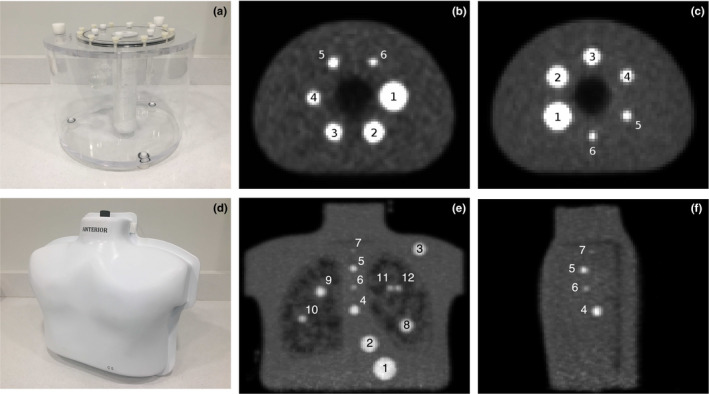
Examples of image quality phantoms and insert numbering scheme used in this work. (a) Photo of NEMA phantom. (b) Axial slice of PET scan of the NEMA phantom showing insert numbering scheme. (c) Example of the NEMA phantom with different insert positions than in (b). (d) Photo of SNMMI/CTN phantom. (e) PET intensity projection image showing all inserts in SNMMI/CTN phantom. (f) Center sagittal slice of PET scan for SNMMI/CTN phantom showing inserts 4–7. [Color figure can be viewed at wileyonlinelibrary.com]

Table 1.

Description of spherical inserts in the two IQ phantoms

Insert label	Interior diameter	Background region	Present in
			NEMA	CTN
1	37 mm	Standard contrast	Yes	Yes
2	28 mm	Standard contrast	Yes	Yes
3	22 mm	Standard contrast	Yes	Yes
4	17 mm	Standard contrast	Yes	Yes
5	13 mm	Standard contrast	Yes	Yes
6	10 mm	Standard contrast	Yes	Yes
7	7 mm	Standard contrast	No	Yes
8	22 mm	High contrast	No	Yes
9	17 mm	High contrast	No	Yes
10	13 mm	High contrast	No	Yes
11	10 mm	High contrast	No	Yes
12	10 mm	High contrast	No	Yes

2.A. NEMA NU‐2 IQ Phantom

The NEMA phantom has six spherical inserts with diameters ranging from 10 to 37 mm arranged in a circular pattern. Inserts are labeled 1 to 6, starting with the largest insert [Fig. 1(b)]. All inserts are located in a uniform background with a lower concentration of tracer. For the purpose of this work, all inserts are filled with tracer solution 9.7:1 activity ratio over background. This activity ratio is used both by EARL⁹ and the National Cancer Institute reconstruction harmonization initiative. Automated analysis methods have been proposed for the NEMA phantom. Bergmann et al.¹⁰ utilized an automated analysis approach for the NEMA NU‐2 2001 protocol.¹² Their approach registers a standard contour of the inside of the phantom body to the contour taken from the center slice of the CT image. No publication was found that validates their method. Pierce et al.¹¹ developed and validated an automated analysis algorithm for the EARL protocol. Their approach starts by estimating the centers of the three largest spheres in the PET image. These centers are transferred to the CT image and refined using a hollow sphere template filter in a local region around each center. The centers of the smallest three spheres are estimated using the known arrangement of inserts in the phantom and then refined using the same filter method in CT. All six centers are transferred back to the PET volume and refined to best fit the PET data. Thus, their approach relies on visible insert walls in CT. Such an approach can be problematic with thin insert walls or insert walls with nearly equivalent radiodensity to water.

2.B. SNMMI/CTN phantom

A newer image quality phantom with a more complex and clinically relevant design is the SNMMI/CTN chest oncology phantom. Six of the twelve inserts in the CTN phantom are identical in size to the inserts in the NEMA phantom and situated in a uniform background similar to conditions in the NEMA phantom. The remaining inserts are either smaller, situated in close proximity to another insert, or located in a low concentration region, simulating lung tissue. Inserts 1–7 are located in the uniform region of the phantom [Fig. 1(e)]. The remaining spheres, 8–12, are located in the lung regions of the phantom where the tracer solution is partially displaced by styrofoam inserts to simulate lung densities. This results in a higher contrast between insert and background. The 7 mm sphere (insert 7) is designed as a lesion detectability challenge. Another challenge is the ability to separate the two 10 mm lung spheres (inserts 11 and 12) in close proximity. Programmatically, the CTN phantom spheres are filled at a 4:1 insert to background activity ratio in uniform regions. In this study, both a 4:1 and 2:1 activity ratio were used to challenge the automated segmentation algorithm. Therefore, the CTN phantom data are more challenging in regard to object detection, resolution, and contrast recovery than the NEMA phantom data. Moreover, the material of the hollow spheres in the CTN phantom has a radiodensity that is almost identical to that of water. Because of this, the insert walls are nearly invisible in CT, forcing analysis of inserts to mainly rely on the PET scan. To our knowledge, no automated analysis approach currently exists for the newer CTN phantom.

3. Image data

A diverse set of PET phantom scans were utilized to develop and validate the proposed approach. A total of 54 PET phantom scans were used for method development (development set). A separate set of 35 scans was used for validation (validation set). Table 2 summarizes the image characteristics of both sets. Image data were collected as part of the NIH NCI project R01CA169072. Figure 2 shows some examples of CTN phantom images. Low contrast and high noise make manual analysis difficult in some cases. Also, the corresponding CT image [Fig. 2(c)] does not reveal insert wall locations, as the radiodensity of the plastic is nearly identical to water.

Table 2.

Summary of phantom PET scans used in this work. Value ranges are described as minimum and maximum with median value in parentheses

	Development set			Validation set
	NEMA 9.7:1	CTN 4:1	CTN 2:1	NEMA 9.7:1	CTN 4:1	CTN 2:1
Scans	25	17	12	15	10	10
Institutions	6	1	1	5	2	1
Manufacturers	Siemens	Siemens	Siemens	Siemens	Siemens	Siemens
	GE			GE	GE
	Philips			Philips
Different scanner models	7	1	1	5	3	2
Background	768–2061	5389–6326	7278–8689	767–2062	4502–6195	3411–5749
Activity [Bq/ml]	(1292)	(5741)	(7625)	(1640)	(4885)	(4940)
Pixel Size [mm]	2.673–4.073	3.394	3.394	2.734–4.073	3.394–4.073	3.394
	(2.673)			(3.394)	(3.394)
Slice	2.025–5.000	2.025–2.027	2.027	2.025–4.000	2.025–5.000	2.025–2.027
Thickness [mm]	(2.025)	(2.027)		(3.270)	(2.027)	(2.027)
Slices	45–81 (81)	171–197 (171)	171	45–81 (47)	83–197 (171)	171–191 (171)
Imaging time [min]	30a	1–6 (4)b	1–6 (3)b	30a	4–6 (4)b	1–6 (2)b
Iterationsa Subsets	42–64 (48)	32–42 (42)	42	24–147 (63)	32–72 (42)	32–42 (42)
Gaussian filter [mm]	3–7 (7)	4–7 (5)	4–7 (5)	3–7 (5)	2–7 (5)	5–7 (5)

^aSingle bed position.

^bPer bed position.

Figure 2.

Examples of coronal CTN phantom slices. (a) Scan using 6 min per bed position with 4:1 activity ratio. (b) Scan with 1 min per bed position with 2:1 activity ratio. (c) Attenuation‐correction CT image for the same slice in (b). Note that insert walls cannot be detected in the CT image.

4. Methods

We developed a fully automated analysis approach that locates and measures inserts inside the phantoms. The method is based on a scale‐space‐based insert detection step, followed by a robust model matching approach. Thus only relevant information (i.e., insert location and relative constellation to other inserts of the phantom) is considered. Compared to using a phantom volume template combined with a simple registration method for aligning the template with the scan to process, our approach has several advantages. First, compared to volume registration, no initialization is required, which is typically performed manually. Thus, our method is deterministic and not prone to getting stuck in local minima. Second, since only relevant image information is utilized, our approach is faster. Third, our approach is better equipped to handle manufacturing tolerances leading to local variation in insert location.

During method development, the development set described in Section 3 was utilized. Before model‐based analysis, a model for each of the two phantom types is created (Section 4.A). Models are utilized to increase the robustness of the insert detection algorithm, which is described in Section 4.B. After the inserts are located, measurements are taken inside spherical ROIs for each insert and several background regions (Section 4.C.)

4.A. Building phantom models

Models of each phantom are utilized to add robustness to the automated analysis approach. Each model consists of a set of labels that represent the phantom inserts. Let a model L be represented by $L=\{l_i|i=1,2,\dots ,n_{\mathit{ROI}}\}$ where l _i represents the label associated with insert i and n _ROI denotes the number of inserts in the phantom. Each label is associated with information about the insert size and relative position of the insert. Let the notation s(l _i ) represent the size (diameter) of insert i and let d(l _i ,l _j ) represent the Euclidean distance between insert i and another insert j.

Manufacturing tolerances during construction of the phantoms cause no two phantoms to be perfectly alike. Moreover, detected center‐to‐center distances of the inserts in the image data can deviate from the expected values. This is due in part to PET reconstruction parameters, center detection inaccuracies, partial volume effects, and noise. Therefore, to build a realistic model, an estimate for the standard deviation of center‐to‐center distance σ _d is required. The methods for determining σ _d and the distances between inserts for the different phantom types are described below.

4.A.1. NEMA NU‐2 IQ phantom model

The inserts of the NEMA phantom follow a known arrangement in a three‐dimensional space. As shown in Figs. 1(b) and 1(c), the position of the inserts can vary among phantom constructions, but the relative distances between insert pairs should not change within a single phantom. The centers of the six inserts are evenly spaced along a circle of radius 57.2 mm. Therefore, relative center distances for the NEMA phantom can be described analytically. This exact calculation does not provide a way to determine the standard deviation of center‐to‐center distances. However, as demonstrated by experiments on the development set, which are summarized in Appendix A, the selection of σ _d is not critical as long as it is not selected too low, because of utilizing a score‐based label assignment algorithm (Section 4.B.3). Consequently, σ _d was set to the same value as determined for the CTN phantom (see below), which is likely somewhat larger as needed for the NEMA phantom.

4.A.2. SNMMI/CTN phantom

While the inserts of the CTN phantom follow a similar pattern among each build of the phantom, the exact locations of inserts within an individual phantom are not precisely known. Thus, the following approach was utilized to measure all insert center locations of multiple phantom instances, and subsequently a mean insert model was built. CT images of five instances of CTN phantoms were available to be segmented to create a mean model. The insert center locations for each CTN phantom instance were determined using a region‐growing segmentation method. Unfilled phantoms were imaged with a Siemens Biograph 64 scanner to produce 512 × 512 × 175 CT volumes having voxel size 0.98 × 0.98 × 2.00 mm. Note that a single scan per CTN phantom on a single CT scanner was used, because the manufacturing process represents the larger source of variability. Empty phantoms were used so that the insert walls were visible [Fig. 3(a)]. The volume was then upsampled to voxel size 0.50 × 0.50 × 0.50 mm using cubic B‐spline interpolation. For insert segmentation, seed points were manually placed in the center of each insert and a region growing algorithm was applied to each empty sphere. The free, open‐source software 3D Slicer^{13, 14} was utilized for region growing. The region‐growing parameters were adjusted to achieve spherical segmentations that completely fill the inside of each insert without leaking outside the insert wall. Figure 3(b) shows a typical example of a segmentation result. After segmentation, the center of each insert was determined by calculating the centroid. All center‐to‐center distances between insert pairs were then calculated. The distance d(l _i ,l _j ) was estimated by averaging the distances between insert center i and j in all five phantoms. Subsequently, the estimate for σ _d was determined by calculating the largest standard deviation of the center‐to‐center distances. Among the five CTN phantoms, the largest standard deviation was σ _d = 2.0 mm and occurred with the distances between inserts 4 and 11.

Figure 3.

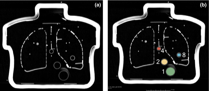
Empty CTN phantom imaged with CT. (a) Coronal slice of empty CTN phantom. (b) Region‐growing‐based segmentation results. In this case, only inserts 1, 2, 4, and 8 are shown. [Color figure can be viewed at wileyonlinelibrary.com]

4.B. Robust insert detection and model fitting

The proposed insert detection algorithm consists of six processing steps. First, the image is preprocessed and intensity values are normalized (Section 4.B.1). Second, candidate detection (Section 4.B.2) locates bright (high uptake) sphere‐like regions in the image volume. Third, label assignment (Section 4.B.3) uses an optimization approach to produce an initial labeling of the insert candidates. Fourth, model fitting (Section 4.B.4) aligns the phantom model to the initial labeling in order to correct a potential mislabeling and/or omissions. Finally, a refinement step (Section 4.B.5) searches a local region around each initial ROI placement to better fit the image data. The model selection step described in Section 4.B.6 is optional and allows for automatically determining the phantom type (i.e., NEMA or CTN phantom) based on the best‐fitting model.

4.B.1. Image preprocessing

To reduce the run‐time and memory usage of the algorithm, the PET image volume is cropped by defining a fixed region around the gray‐value center of mass of the image. Cropping the image volume has the added benefit of eliminating reconstruction artifacts that may occur near the border of the volume. The cropped volume is resampled to a voxel size of 2.0 × 2.0 × 2.0 mm. This voxel size was found to be a good compromise between algorithm run‐time and preserving the details of the image data. The image gray values are then rescaled to be between zero and one.

4.B.2. Insert candidate detection

Detecting the location and sizes of spherical inserts can be accomplished by utilizing a scale‐space approach. The scale‐space approach is a computer vision method that identifies scale‐invariant image features. The approach has many applications, such as edge detection,^{16, 17} corner detection,^{18, 19, 20} and blob detection.^{21, 22} For our application, we utilize a blob detection approach, which identifies bright, sphere‐like structures in the PET volume, generating candidates for the true inserts.

We follow the blob detection approach with automatic scale selection described by Lindeberg.²² Detection of bright blobs is achieved by convolving the input volume with a set of inverted Laplacian of Gaussian (LoG) filters. The Laplacian of a normalized three‐dimensional Gaussian function g(x,y,z) with standard deviation σ is given by

$${\mathrm{\nabla }}^{2}g(x,y,z)=\frac{1}{{\mathit{\sigma }}^5{(2\mathit{\pi })}^{3/2}}\left(\frac{x^2+y^2+z^2}{{\mathit{\sigma }}^2}-3\right)e^{\frac{-(x^2+y^2+z^2)}{2{\mathit{\sigma }}^2}}.$$ (1)

The zero‐crossings of the LoG filter form a sphere. When the filter has zero‐crossings that match the diameter of a spherical insert in the image volume, the response of the filter will have a local maximum at the center of the insert. Because the insert sizes are known, the set of diameters Θ for the LoG filters was chosen to be Θ = {10,13,16,…,37} in millimeters. In Eq. (1), the relationship between σ and the diameter ${\mathit{\theta }}_i\in \mathrm{\Theta }$ is $\mathit{\sigma }={\mathit{\theta }}_i/\sqrt{6}$. Note that the 7 mm scale is omitted from set Θ, because this diameter is small with respect to the sampling grid and very sensitive to image noise. Also, the scale space is typically generated for a set of discrete scales to reduce memory and computational requirements. Despite the utilization of discrete scales, which might not be identical to the actual object size, scale space‐based approaches are quite robust and the discrete scale closest to the true object size will likely be selected. In our case, we utilize a spacing of 3 mm between discrete scales, which is quite dense. Because the algorithm is cost based, a mismatch between discrete scales and actual object size are robustly handled.

Candidates are selected by finding local maxima among all filter responses. The global maximum is first selected and its coordinates, scale, and response value are recorded. The region around this maximum is suppressed across all scales to avoid reselecting the structure corresponding to this maximum. A new global maximum is selected as a candidate and the process repeats until a total of n _LM local maxima are identified. Let $C=\{c_n|n=1,2,\dots ,n_{\mathit{LM}}\}$ represent the set of detected insert candidates, where c _n represents the n‐th candidate. To ensure most of the true inserts are selected as candidates, we select n _LM = 24 candidates, which is ≥2n _ROI for both phantoms considered in this work. Note that if only processing of NEMA phantom is considered, n _LM = 12 would be sufficient. Each insert candidate has information about its size and position, similarly to how labels in the model are described (Section 4.A). Let the notation s(c _n ) represent the detected size (scale) of the n‐th candidate and let d(c _n ,c _m ) represent the Euclidean distance between the n‐th and m‐th candidates.

Local maxima can occur in regions that do not correspond to actual inserts in the phantom, for example, regions near the outer edge of the phantom. In order to penalize regions near the edge of the phantom, all values below 0.05 in the normalized image from Section 4.B.1 are set to 0.05 before applying the LoG filters. This threshold value was found to work well for all phantom contrast ratios considered in this work.

Figure 4 shows the scale‐space responses of two different LoG filters. A local maximum occurs at the center of the largest insert in the 37 mm scale. Another local maximum occurs at the center of insert 4 in the 16 mm scale. Note that the actual size of insert 4 is 17 mm (see discussion of discrete scales above). Similarly, partial volume effects and effects of cold insert walls²³ can lead to deviations of selected scale maxima. We, therefore, introduce a scale tolerance parameter σ _s that will be used during label assignment in Section 4.B.3. Similar to how σ _d is a tolerance for the center‐to‐center distances of the inserts, the parameter σ _s is a tolerance for the scale at which a candidate is detected. For the proposed approach, the value of σ _s was set to 6 mm. This allows an insert with diameter ${\mathit{\theta }}_i\in \mathrm{\Theta }$ to be detected at adjacent scales without severe penalty in the label assignment step, which is described in the next section.

Figure 4.

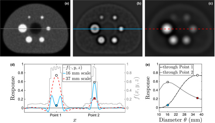
Illustration of scale‐space insert candidate detection approach. (a) Axial slice of input volume f. Intensity profiles are determined along the line through inserts 1 and 4 as shown. The scale space responses at the same slice are shown for (b) 16 mm and (c) 37 mm filters. (d) Line intensity profiles through inserts 1 and 4 for images (a)–(c). (e) Scale‐space profiles at Point 1 (circle) and Point 2 (square). White markers indicate local maxima in scale space. [Color figure can be viewed at wileyonlinelibrary.com]

4.B.3. Label assignment

To fit the model to the detected inserts (Section 4.B.4), an initial labeling is required. Because n _LM is greater than the total number of inserts, some candidates do not correspond to an actual phantom insert. For this reason, a score‐based label assignment algorithm is used to assign the best labeling to candidates according to their size and relationship to other candidates. Scores are determined for all combinations of labels and candidates, resulting in a score matrix S of size n _LM ×n _ROI . The task then becomes an optimal assignment problem, which is solved by using the Hungarian algorithm.²⁴ The algorithm selects one candidate (row) for each label (column) in S such that the total score is maximized.

The elements S(n,i) of matrix S are calculated as follows. First, a candidate $c_n\in C$ is selected and given the label $l_i\in L$. Other candidates and model information (Section 4.A) are then utilized to build evidence to support the assumption that the correct label for c _n is l _i . For this purpose, an evidence matrix E _n,i of size (n _LM −1)×(n _ROI −1) is built by evaluating evidence for relations between c _n and all other candidates c _m with m = 1,2,…,n _LM and m≠n. Because labels are not known, all possible combinations of relations between c _m and label l _j with j = 1,2,…,n _ROI and j≠i are evaluated. A relation r consists of three parts: the detected size of candidate c _n , the detected size of candidate c _m , and the distance between them d(c _n ,c _m ). The evidence of a relation supported by the model between candidate pair 〈c _n ,c _m 〉 and model pair 〈l _i ,l _j 〉 is determined using the equation r(〈c _n ,c _m 〉,〈l _i ,l _j 〉) = ξ(s(c _n ),s(l _i ),σ _s )ξ(s(c _m ),s(l _j ),σ _s )ξ(d(c _n ,c _m ),d(l _i ,l _j ),σ _d ), which compares detection evidence to information from the model. The Gaussian scoring function ξ penalizes relations that deviate from the model. It is defined by $\mathit{\xi }(x,\mathit{\mu },\mathit{\sigma })=e^{\frac{-{(x-\mathit{\mu })}^2}{2{\mathit{\sigma }}^2}}$, where x represents an observed value (candidate), μ is the expected value (model), and σ controls the penalty for deviating too far from μ. Figure 5 illustrates the evaluation of three relations of candidates for one pair of labels in the model. An element of E _n,i is calculated as E _n,i (m,j) = r(〈c _n ,c _m 〉,〈l _i ,l _j 〉). After all relations are evaluated for a fixed n and i, the maximum evidence that c _n is label l _i is determined by applying the Hungarian algorithm to E _n,i . This produces the subset of candidates that provide the largest support for assigning label l _i to candidate c _n . The total evidence score from these candidates are added together and is assigned to element S(n,i) of the score matrix. The algorithm continues to score all candidates in this way for n = 1,2,…,n _LM and i = 1,2,…,n _ROI . As stated above, the subset of candidates that maximize the label assignment scores of S are chosen and further analyzed in the next step.

Figure 5.

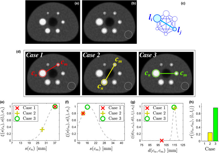
Illustration of evaluating candidate relations. (a) Axial slice of image volume showing all inserts. (b) Detected insert candidates, including an outlier near the edge of the phantom. (c) A label pair 〈l _i , l _j 〉 is selected from the model and assigned to 〈c _n , c _m 〉. (d) Examples of candidate relations, with Case 3 being the correct relation. (e) Scores for size of c _n . (f) Scores for size of c _m . (g) Scores for distance between c _n and c _m . (h) Overall evidence that 〈c _n , c _m 〉 represents 〈l _i , l _j 〉 for relations in (d). Note that Case 3 receives the highest score. [Color figure can be viewed at wileyonlinelibrary.com]

4.B.4. Robust model fitting

The insert candidate detection step can fail to detect small inserts, especially in very noisy PET scans. Moreover, the initial labeling may contain incorrectly labeled inserts and/or assign labels to outliers. To address these issues, a robust model fitting step is performed. First, the model is rigidly aligned to the labeled insert candidates, and the goodness of fit is checked by using the maximum distance error E _d between candidates and their corresponding center location in the aligned model. Thus, a mislabeling will result in a large value for E _d . Therefore, if E _d ≥ 5 mm, then the algorithm iteratively attempts to improve model alignment by using a backward elimination approach. The backward elimination starts by removing one labeled candidate at a time and determining the subset of candidates that produces the smallest error. If the subset of candidates fit the model with E _d < 5 mm, then that subset of labeled candidates is deemed acceptable. If the distance error is still too high, then two labeled candidates are removed at a time. The algorithm continues increasing the number of candidates removed until an acceptable alignment is found. If less than three candidates remain, the algorithm fails. If a good alignment is found, the candidates that were not used for alignment are replaced by positions and corresponding labels given by the aligned model.

4.B.5. Refinement

After the initial locations of all the inserts have been found, they are refined to achieve subvoxel resolution and a better fit to the input image data. For each insert, a search region is defined around the initial insert center. The region is determined using a search radius, thus limiting the distance that the center can move during refinement. This search radius is equal to the radius of the insert being refined. Because, insert center refinement is voxel based, voxel size is a limiting factor in terms of resolution. Therefore, the search region is upsampled to a resolution of 0.5 × 0.5 × 0.5 mm to gain subvoxel resolution. To ensure that the refinement step is robust to noise and nearby bright objects, the image data in the search region are attenuated by a Gaussian function. The Gaussian is centered at the location determined by the fitted model and has standard deviation equal to the inner diameter of the insert. An ideal sphere template filter with the same inner diameter of the insert is created. This filter is the shape of a sphere with voxels inside the sphere equal to one. The position of maximum correlation between the image and the filter is determined and taken as the new coordinates of the insert center.

4.B.6. Model selection

For a given PET scan, the algorithm may optionally select the corresponding phantom model. To use this option, two or more phantom models need to be provided to the algorithm. In Appendix B, we provide an example algorithm for selecting between NEMA and CTN phantoms.

4.C. Uptake measurement

For each detected insert, a spherical measurement region (ROI), which matches the insert size, is defined in the original input volume (Fig. 6). Several quantitative indices are determined for each ROI. Intensity‐based measurements are recorded in units of standardized uptake value (SUV). Three indices were utilized for validation of the automated approach: SUV _max , SUV _peak , and SUV _mean . SUV _max is the most common index for quantitative PET analysis and depends the least on the placement of the ROI. SUV _peak is a more robust alternative to SUV _max and is defined as the maximum average SUV calculated from a 1 cm³ sphere placed within the ROI.¹ SUV _mean is the average of all voxels contained within the ROI. Therefore, its value is more sensitive regarding ROI placement. To deal with partial volume effects during uptake measurement, we perform the calculation of the exact partial volumes using the equations described by Tengattini and Andò.²⁵

Figure 6.

Examples of automated detection results. (a) NEMA phantom at 9.7:1 contrast. (b) CTN phantom at 4:1 contrast. (c) CTN phantom at 2:1 contrast. Note that (b) and (c) are intensity projections of the coronal view in order to visualize all inserts. In addition to the ROIs (solid circles) covering the inserts in the phantom, one or several background ROIs (dashed circles) can also be placed automatically inside the phantom relative to the inserts, allowing for normalization of insert uptake values. [Color figure can be viewed at wileyonlinelibrary.com]

5. Experimental setup

The proposed automated analysis approach (Auto) was applied to the validation set described in Section 3. Scans were categorized by imaged phantom type and contrast level: NEMA phantom at 9.7:1 contrast (NEMA 9.7:1), CTN phantom at 4:1 contrast (CTN 4:1), and CTN phantom at 2:1 contrast (CTN 2:1). For comparison, the phantom images were also analyzed by four expert image analysts (Manual). For this purpose, an in‐house extension of 3D Slicer was utilized for manual ROI placement. The software allows for placing regions anywhere throughout the volume and is not limited to the voxel centers. Each expert manually placed a ROI at each insert location in every phantom PET scan. This approach is commonly used in practice. The sequence of datasets was randomized for each expert to reduce learning effects. After at least one day, the experts repeated the process using a second randomized sequence, producing a total of eight ROIs for every insert. The ROI labels, ROI center coordinates, analysis time, and insert measurements were recorded for the automated method and manual approach.

The proposed algorithm was implemented in C++ and utilizes the Insight Toolkit (ITK)¹⁵ for image processing. Both the Auto and Manual approaches were performed on the same desktop computer with a 3.20 GHz processor and 32 GB of memory.

An independent reference standard was created by two other experts, which used PET and CT scans of the phantoms for ROI placement. This procedure was repeated by both experts, resulting in a total of four ROIs for every insert. The average ROI center location and uptake measurements from these four ROIs were used as reference. It is expected that the experts using both PET and CT information will achieve the most consistent ROI placements. To assess the quality of the independent reference standard, the estimated interoperator and intraoperator variability of the two experts was calculated (see below) and are summarized in Table 3. The overall variability is well below 1 mm for all phantom types and contrast levels, confirming the quality of the independent reference standard.

Table 3.

Estimates for interoperator and intraoperator variability of the independent reference standard. Estimates are posterior means with 95% credible intervals in brackets

Phantom	Contrast	Variability of reference (mm)
		Interoperator	Intraoperator	Overall
NEMA	9.7:1	0.32 [0.27, 0.37]	0.39 [0.36, 0.41]	0.50 [0.47, 0.53]
CTN	4:1	0.30 [0.23, 0.36]	0.56 [0.53, 0.58]	0.63 [0.60, 0.66]
CTN	2:1	0.34 [0.26, 0.41]	0.64 [0.61, 0.67]	0.72 [0.69, 0.76]

The proposed approach was evaluated regarding its ability to correctly detect the inserts in a PET phantom scan based on the following three criteria.

5.A. Model selection correctness

The automated approach has the option to select the best‐fitting model after being given multiple models (i.e., NEMA NU‐2 and CTN oncology phantom) as input. This feature is assessed for correctness by determining if the analysis approach selected the model of the underlying phantom.

5.B. Label correctness

The correct label number must be assigned to each ROI to achieve correct measurements and allows for comparisons across multiple PET phantom experiments. The proposed approach was assessed for ROI label accuracy by manually inspecting the labels generated by the automated approach.

5.C. Center detection accuracy

Each ROI needs to be placed such that it completely covers the insert in the PET image data. It is assumed that the experts can place each ROI with reasonable accuracy. Furthermore, insert center positions were obtained in our study on the same set of images from different operators, on multiple occasions, and with different methods; resulting in repeated measurements. To account for correlation induced by the repeated nature of our data and to simultaneously estimate bias and variability for the automated and manual methods relative to the independent reference, statistical analysis was performed with mixed‐effects regression models, as described in Appendix C.

The measurements obtained from the proposed analysis approach and the manual approach were compared with the average measurements from the independent reference standard. The metrics SUV _max , SUV _peak , and SUV _mean were tested for correlation with the reference using Bland–Altman plots for percent difference. Correlation of these metrics is further tested using least‐squares regression.

6. Results

The automated approach selected the correct model for all 35 test phantom datasets. Moreover, the automated approach determined the correct label for all 330 inserts in all 35 phantom datasets. Figure 6 shows typical results of the proposed approach. ROIs for inserts as well as background regions are automatically placed in the image volume as shown. Figure 7 shows axial, sagittal, and coronal detail views of the inserts detected in Fig. 6.

Figure 7.

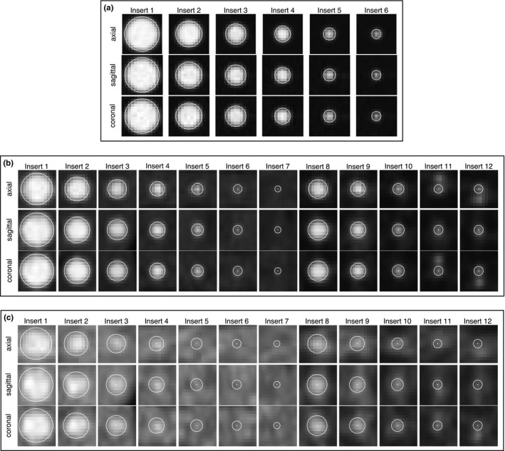
Detail views of detected inserts. Spherical ROIs and their centers are indicated in white. (a) Inserts from NEMA phantom [Fig. 6(a)] at 9.7:1 contrast. (b) Inserts from CTN phantom [Fig. 6(b)] at 4:1 contrast. (c) Inserts from CTN phantom [Fig. 6(c)] at 2:1 contrast.

Figure 8 shows the center detection root‐mean‐square error (RMSE) per insert for each method. Mean‐square error (MSE) is the sum of the bias squared and total variance of the method around each insert. MSE has units in millimeters squared, so RMSE is reported to enable intuitive interpretation. Table 4 shows the bias, standard deviation, and RMSE of each method without controling for inserts. Although Fig. 8 displays the insert‐specific RMSE estimates and individually compares the differences between methods, the RMSE estimates in Table 4 are averaged over the inserts to provide an aggregate view of the differences. Thus, the table shows how much the automated method error is lower than the manual method on average. Furthermore, the table additionally provides the separate bias and variability (standard deviation) components that make up the RMSE. From the components, similar amounts of bias and variability can be seen to contribute to the overall manual error. On the other hand, the automated method is deterministic and therefore has zero variability. In addition, bias alone is lower for the automated method compared to the manual.

Figure 8.

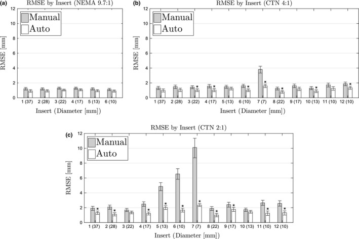
Root‐mean‐square errors for each insert by phantom and contrast. (a) NEMA phantom at 9.7:1 contrast. (b) CTN phantom at 4:1 contrast. (c) CTN phantom at 2:1 contrast. Stars indicate significant difference from manual method.

Table 4.

Estimates for center detection bias, standard deviation (intra‐ and interobserver variability), and RMSE in millimeters by method. Estimates are posterior means with 95% credible intervals in brackets. Bold values indicate significant difference from manual method

	Phantom	Contrast	Error of method (mm)
			Bias	Std. Deviation	RMSE
Manual	NEMA	9.7:1	1.08 [1.00, 1.14]	0.55 [0.53, 0.57]	1.21 [1.15, 1.27]
	CTN	4:1	1.46 [1.37, 1.54]	1.04 [1.01, 1.06]	1.79 [1.72, 1.86]
	CTN	2:1	2.80 [2.62, 2.97]	2.89 [2.81, 2.97]	4.03 [3.89, 4.18]
Auto	NEMA	9.7:1	0.97 [0.91, 1.03]	0	0.97 [0.91, 1.03]
	CTN	4:1	1.12 [1.06, 1.16]	0	1.12 [1.06, 1.16]
	CTN	2:1	1.48 [1.41, 1.55]	0	1.48 [1.41, 1.55]

Figures 9, 10, 11 show the Bland–Altman plots of SUV _max , SUV _peak , and SUV _mean , respectively, for the manual and automated methods. The percent difference of the measurement produced by each method was plotted against the average of the reference and method measurements. Plotting the data in this way illustrates any potential bias in the measurements and dependence on SUV level. In addition, a least‐squares regression fit was determined for the measurements from all eight manual trials and the automated method. Correlation with the reference was estimated using the R ² value, which is given in Figs. 9, 10, 11 for each method and phantom analyzed.

Figure 9.

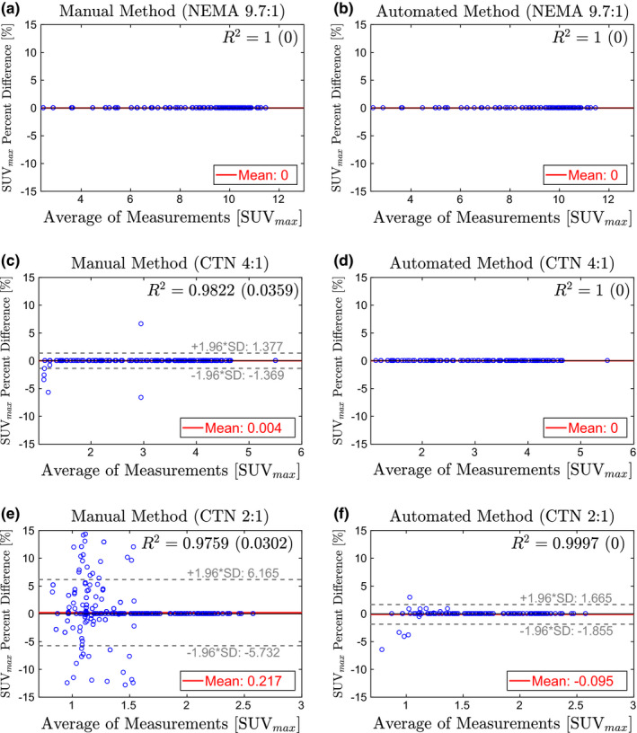
Bland–Altman plots comparing SUV _max from the manual method (left column) and automated method (right column) to the reference standard. Estimates for R ² are given as the average of all trials with the standard deviation in parentheses. (a)–(b) NEMA phantom at 9.7:1 contrast. (c)–(d) CTN phantom at 4:1 contrast. (e)–(f) CTN phantom 2:1 contrast. [Color figure can be viewed at wileyonlinelibrary.com]

Figure 10.

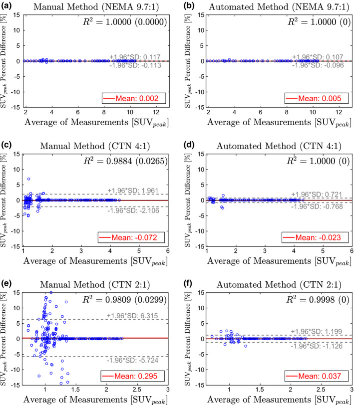
Bland–Altman plots comparing SUV _peak from the manual method (left column) and automated method (right column) to the reference standard. Estimates for R ² are given as the average of all trials with the standard deviation in parentheses. (a)–(b) NEMA phantom at 9.7:1 contrast. (c)–(d) CTN phantom at 4:1 contrast. (e)–(f) CTN phantom 2:1 contrast. [Color figure can be viewed at wileyonlinelibrary.com]

Figure 11.

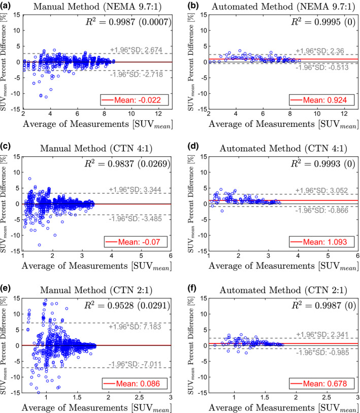
Bland–Altman plots comparing SUV _mean from the manual method (left column) and automated method (right column) to the reference standard. Estimates for R ² are given as the average of all trials with the standard deviation in parentheses. (a)–(b) NEMA phantom at 9.7:1 contrast. (c)–(d) CTN phantom at 4:1 contrast. (e)–(f) CTN phantom 2:1 contrast. [Color figure can be viewed at wileyonlinelibrary.com]

The automated method was found to be significantly faster compared to the manual approach (p≪0.001). The required processing time a for a single dataset with the automated method was 30.6 s, on average. In comparison, The manual approach required 247.8 s, on average.

7. Discussion

7.A. Performance

For all phantoms and contrast situations tested, the proposed automated method showed significantly lower center detection RMSE than the manual approach (Table 4). In this context, a major advantage of the automated method is that it has no variability due to its deterministic nature and is therefore desirable for many applications like quality control. When comparing the bias, automated and manual methods showed similar performance on the NEMA 9.7:1 phantom, which has the highest contrast, and therefore, is easy to analyze manually. In both cases, the bias is well below the size of a voxel. Differences in bias become significant for the CTN phantom, which is more challenging to analyze manually due to lower contrast, smaller inserts, and more challenging insert constellations. Especially in the case of a contrast ratio of 2:1, the bias introduced by manual analysis approaches the median voxel size, while the automated method roughly shows half the bias. When comparing individual inserts (Fig. 8), the same trend can be observed. In addition, one can notice that certain inserts are more difficult to locate manually due to small size paired with low local contrast (i.e., inserts 5, 6, and 7). Figure 12 illustrates this situation by depicting the ROI placements for inserts 5 and 6 in a CTN phantom with 2:1 contrast. The bright structures visible in the corresponding CT images are the insert fill tubes. The true location of the insert is somewhere between the ends of these tubes. The manual approach shows the highest variability, which is quite often paired with low accuracy, especially for small inserts. Despite the limited information available in the PET scan and the presence of an air bubble in the case of insert 6, the automated method places the ROI with lower error.

Figure 12.

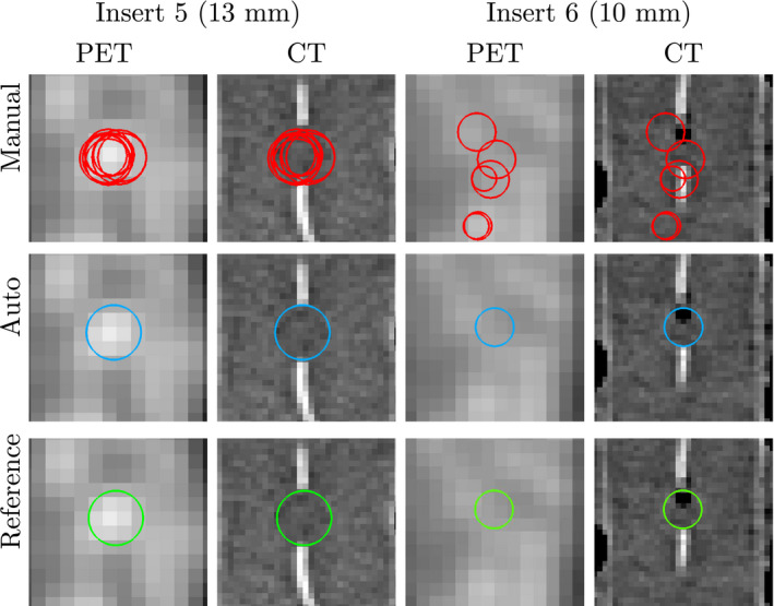
ROI placements for manual method (top row), automated method (center row), and reference (bottom row) for two inserts in a CTN phantom at 2:1 contrast. Images are axial views at the center of the insert. Note that the centers of the ROIs may be in different slices than the ones shown. [Color figure can be viewed at wileyonlinelibrary.com]

Of all three investigated uptake indices, SUV _max depends the least on the placement of the measurement ROI (i.e., center detection accuracy). In contrast, SUV _mean is the most sensitive measurement. SUV _max measurements on the NEMA 9.7:1 phantom show no errors for both methods [Figs. 9(a) and 9(b)]. In the case of the automated method, there is no change in performance on the CTN 4:1 phantom [Fig. 9(d)], while some errors in SUV _max measurement are noticeable for the manual approach [Fig. 9(c)]. On the CTN 2:1 scans, both methods show some errors [Figs. 9(e)] and 9(f)], with mean and 95% intervals the lowest for the automated method. Note that CTN 2:1 is typically not utilized in practice and was included to test the limits of methods. A similar trend is observable for SUV _peak (Fig. 10) and SUV _mean (Fig. 11) measurements on all phantoms — 95% intervals are tighter and expand less with decreasing contrast ratio. Also, inserts with lower SUV tend to have larger percent differences for the manual method. This is apparent in the cone shape of the Bland–Altman plots. In comparison, the results of the automated method show much less dependence on SUV level. This trend is also reflected in the R ²‐values in Figs. 9, 10, 11. Across phantoms, the automated method maintains a high correlation (R ² ≥ 0.9987) with the reference. In comparison, the manual approach is more dependent on contrast.

The Bland–Altman plots for the automated approach on SUV _mean measurements (Fig. 11) indicate a small positive bias (< 1.1%), suggesting that SUV _mean values derived by the automated approach are slightly higher on average than the reference. This can be explained by the utilized refinement step (Section 4.B.5), which updates the placement of the ROI based on maximum correlation with an ideal sphere. Consequently, the refinement step maximizes the SUV _mean value of a ROI.

The proposed method was designed to handle arbitrary phantom orientations relative to the PET scanner. The following experiment demonstrates this ability. To simulate a phantom being scanned at different orientations, a single 4:1 contrast CTN phantom scan from the test set was selected that had a voxel size close to median voxel size of PET scans in the test set (Table 2). Subsequently, four different geometric transformations (i.e., rotations) were applied to the PET scan, resulting in four transformed PET volumes (Fig. 13). Then, the algorithm was applied to all four transformed scans, and the automatically measured SUV _max values were compared with that measured by an expert on the same data. The algorithm successfully detected and labeled all inserts, and the algorithm‐generated SUV _max values matched the reference for all inserts. Note that SUV _max is currently utilized for generating plots like the one depicted in Fig. 14. Also, due to the transformation and implied resampling of the PET scan volume, small differences between the plots in Fig. 13 can be observed.

Figure 13.

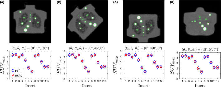
Coronal maximum intensity projections of digitally transformed (rotated) phantom scans and corresponding analysis results. Images were transformed by rotating (a) 180^∘ about the z–axis, (b) 45^∘ about the y–axis, (c) 180^∘ about the y–axis, (d) 45^∘ about the x–axis. [Color figure can be viewed at wileyonlinelibrary.com]

Figure 14.

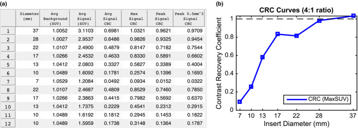
Example of an automated phantom analysis report. (a) Summary table of quantitative indices for a phantom. (b) Corresponding CRC curve for the same phantom. [Color figure can be viewed at wileyonlinelibrary.com]

7.B. Impact

An automated, deterministic phantom analysis method for common PET image quality phantoms is highly desirable to meet current and future clinical trial as well as practice quality control standards. The proposed method analyzes phantoms faster, with no variability, and with less error compared to manual analysis using identical PET image information. In addition, the automated method is suitable for batch processing of many phantom datasets, making it ideal for efficient centralized phantom‐based PET/CT scanner validation for clinical trials as well as to meet new phantom‐based diagnostic imaging standards for PET/CT imaging recently issued by the Joint Commission.²⁶

Our method was developed with the capability to generate automatic phantom reports for quality control and clinical trial qualification. Figure 14 shows examples of a subset of measurements designed to be included in such a report. After the algorithm detects all inserts in the phantom, measurements are taken at each insert as well as background regions inside the phantom (Fig. 6). Background regions are used to assess noise characteristics and, in combination with the insert measurements, generate contrast recovery coefficient (CRC) curves. CRC curves are a standard quantitative measure of scanner/reconstruction performance through characterization of partial volume effects. CRCs are a measure of image quality and are defined as the ratio of measured insert‐to‐background activity ratio to actual insert‐to‐background activity ratio. Analysts can then use such automatically generated standardized reports to meet either clinical trial quality control reporting requirements or as evidence of scanner quality control regulatory compliance. In addition, it is possible to automate the acceptable thresholds for trial qualification and hence provide institutions immediate feedback and thereby enable rapid intervention so that qualification can be achieved. A user could then only submit for formal qualification for study participation after knowing that acceptable thresholds were achieved.

7.C. Limitations and future work

In its current form, our algorithm is limited to phantoms with spherical inserts exclusively. To support phantoms with other insert shapes (e.g., ellipsoidal), the scale‐space detection approach needs to be expanded accordingly. In addition, it is likely that the proposed approach could achieve even higher accuracy by incorporating CT image information into the detection and/or refinement steps. Note that such an approach will likely be phantom‐specific. For instance, the refinement step proposed by Pierce¹¹ could be used as the last processing step for NEMA phantoms. However, this type of refinement will not work on the CTN phantom, because the insert walls are typically invisible in CT. An alternate refinement approach for the CTN phantom could search for the fill tubes and restrict the placement of the ROI to fall somewhere between the ends of the tubes.

8. Conclusions

We have presented an automated model‐based approach for analysis of the NEMA and CTN image quality phantoms PET scans. The approach is generalizable and suitable for similar phantoms with spherical inserts. Validation of the approach showed that the proposed method has less inter‐ and intraoperator variability, has better agreement with an independent reference standard, and is also faster than a manual analysis approach. In the future, we plan to use our automated approach for phantom analysis in PET standardization and harmonization studies.

Conflict of interest

The authors have no conflict of interest to report.

Appendix A.

Impact of model parameter selection

Our approach to insert detection and model fitting is based on a score‐based approach that avoids utilizing hard thresholds. This leads to robustness regarding parameter selection in terms of overall performance. For example, σ _d for the NEMA phantom was estimated to be of similar magnitude as σ _d measured for the CTN phantom. Using the available development set, which 25 scans of six instances of NEMA phantoms allows us to study the impact of selecting σ _d on overall performance. Figure 15 depicts the number of passed (i.e., all inserts were detected and all labels were assigned correctly) cases in percent as a function of model parameter σ _d . As the plot shows, over a wide value range, algorithm performance is not affected by the selection of this parameter. Only if σ _d is selected too low (i.e., too tight distance tolerance), performance degrades, which is expected, but overall still stays quite high (> 90%).

Figure 15.

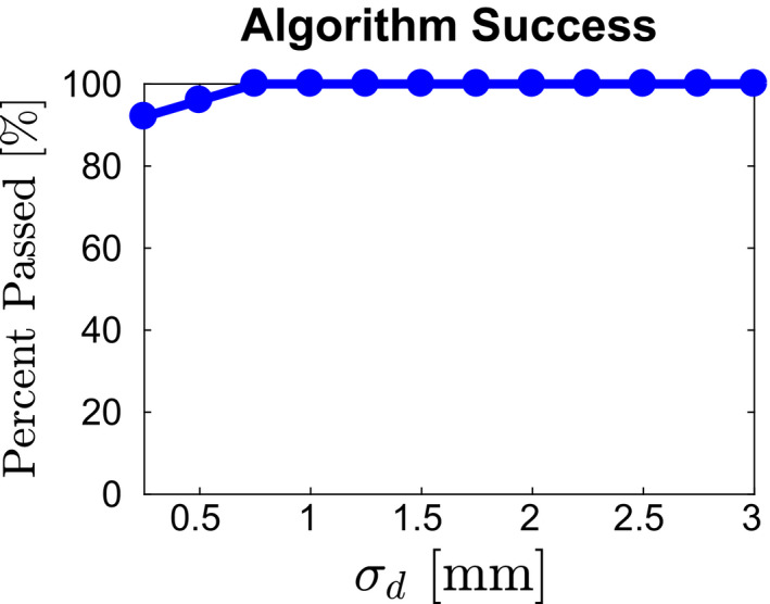
Impact of parameter σ _d on overall method performance. [Color figure can be viewed at wileyonlinelibrary.com]

Appendix B.

Model selection

If two or more different phantoms with spherical inserts need to be analyzed, the following algorithm can be used, assuming that a model is available for each phantom. The corresponding phantom model is determined by evaluating the confidence score c = c _label c _model c _meas and selecting the model with the highest overall confidence. The confidence is an indicator that the phantom model is correct. The individual confidence components are described in detail below.

1. Labeling score confidence c _label measures how well the label assignment (Section 4.B.3) matches the labeling of a phantom model. A similar approach as described in Section 4.B.3 is used to calculate c _label . However, this time only the first six labels are evaluated. This allows for a fair comparison between NEMA and CTN phantom types. All inserts of the NEMA phantom are evaluated, and only the six largest inserts of the CTN phantom located in the “standard contrast” region are evaluated (Table 1), which are matching in size. All possible relations among the six inserts are considered to determine c _label . We define $c_{\mathit{label}}=\frac{1}{6}{\sum }_{i=1}^6\frac{1}{5}{\sum }_{j=1;j\ne i}^{6}r(⟨c_i,c_j⟩,⟨l_i,l_j⟩)$, where 〈c _i ,c _j 〉 represents the candidate pair assigned to label pair 〈l _i ,l _j 〉. The equation for c _label produces a number between zero and one, and a number close to one indicates a good match between the labeling and model.

2. Model fit confidence c _model measures how well the detected centers align with a given model (Section 4.B.4). Its value is dependent on the distance error of aligning the model and n _used , representing the number of candidates that were utilized during model placement. We define $c_{\mathit{model}}=(1-\frac{E_d}{10})\frac{n_{\mathit{used}}}{n_{\mathit{ROI}}}$. If the input model is successfully aligned using the method in Section 4.B.4, it follows that 0 ≤ E _d < 5 and 3 ≤ n _used ≤ n _ROI and therefore 0 < c _model ≤ 1. If the input model cannot be aligned, then c _model is set to zero by default.

3. Measurement confidence c _meas indicates how well the placed ROIs cover bright regions of the PET volume. Therefore, the mean intensity value $\overline{u}$ within each ROI is determined. Again, only the first six inserts are evaluated to ensure a fair comparison. We define $c_{\mathit{meas}}=\frac{1}{6\tilde{u}}{\sum }_{i=1}^6{\overline{u}}_i$, where ${\overline{u}}_i$ is the mean intensity value in insert i and the normalizing factor $\tilde{u}$ is the largest mean observed across all input phantom models. If c _meas is close to one, then the ROI placement is likely covering bright regions in the image.

Appendix C.

Mixed‐effects models for center detection accuracy assessment

Positions obtained on one insert were modeled as follows. We index each method m = 1,2,3 as the automated method, manual method, and independent reference, respectively. Let p _mdijk denote a position identified with method m in dimension d = 1,2,3 for phantom image i = 1,…,I and by operator j = 1,…,J _m on occasion k = 1,2. Systematic and random variations in these positions were assessed with linear mixed‐effects models of the form

$$\begin{array}{cc}\hfill p_{\mathit{mdijk}}& ={\mathit{\mu }}_d+{\mathit{\varphi }}_{\mathit{mdi}}+{(\mathit{\varphi }\mathit{\omega })}_{\mathit{mdij}}+{\mathit{ϵ}}_{\mathit{mdijk}}\hfill \\ \hfill {({\mathit{\varphi }}_{1di},{\mathit{\varphi }}_{2di},{\mathit{\varphi }}_{3di})}^{\top }& \sim N_3(\mathbf{0},{\mathbf{\Sigma }}_{{\mathit{\varphi }}_d})\hfill \\ \hfill {(\mathit{\varphi }\mathit{\omega })}_{\mathit{mdij}}& \sim N(0,{\mathit{\sigma }}_{{(\mathit{\varphi }\mathit{\omega })}_m}^2)\hfill \\ \hfill {\mathit{ϵ}}_{\mathit{mdijk}}& \sim N(0,{\mathit{\sigma }}_{{\mathit{ϵ}}_m}^2),\hfill \end{array}$$

where μ _d represent overall dimension‐specific mean effects, ϕ _mdi are random deviations in the image‐specific means, (ϕω) _mdij are interoperator deviations, and ϵ _mdijk are intraoperator deviations. Likewise, ${\mathit{\sigma }}_{{(\mathit{\varphi }\mathit{\omega })}_m}^2$ and ${\mathit{\sigma }}_{{\mathit{ϵ}}_m}^2$ represent inter‐ and intraoperator variances, respectively. Note that these two variances were fixed at zero for the automated method (m = 1) since its positions are deterministic for a given image. Covariance matrices ${\mathbf{\Sigma }}_{{\mathit{\varphi }}_d}$ capture variability in the scanner placement of phantoms as well as correlation due to the application of methods to the same set of phantom images. The model assumes no correlation between positional directions and that operator variability is the same in all directions. All inserts from a phantom type and scan condition were additionally analyzed together by letting i index all combinations of inserts and images involved. Variability and bias (accuracy) estimates are reported from the models. Bias was computed as the average distance error from the reference standard (m = 3); that is, $Bia{s}_m=\frac{1}{I}{\sum }_{i=1}^I\sqrt{{\sum }_{d=1}^3{({\mathit{\varphi }}_{\mathit{mdi}}-{\mathit{\varphi }}_{3di})}^2}.$ A Bayesian statistical approach was taken to fit the specified model and perform inference based on the posterior distribution of all model parameters. Model‐based estimates are reported as posterior means along with 95% credible intervals. The approach was chosen over a traditional frequentist one for two main reasons. The first was so that probability statements could be made about variability and bias measures of interest. In particular, the reported credible intervals can be interpreted intuitively as containing the true values with 95% probability. The second reason was to avoid a need for asymptotic or finite series approximations in the inference. Our Bayesian posterior estimates, including those for nonlinear functions of the model parameters, were computed directly from the posterior distribution with standard (Markov chain Monte Carlo) Bayesian computational methods. Another reason to consider a Bayesian approach is to combine observed data with prior information. Prior information was not generally available for our application. Prior distributions must nevertheless be specified for the Bayesian model. Therefore, to reflect our lack of prior information, we used vague prior distributions in the form of normals for the mean effects, inverse‐gammas for the scalar variances, and inverse‐Wisharts for the covariance matrices. Sensitivity analysis was performed to confirm that inference was unaffected by the priors. The mixed effects analysis was conducted with the R²⁷ and OpenBUGS²⁸ statistical software.

References

- 1. Wahl RL, Jacene H, Kasamon Y, Lodge MA. From RECIST to PERCIST: evolving considerations for PET response criteria in solid tumors. J Nucl Med. 2009;50(Suppl 1):122S–150S. [DOI] [PMC free article] [PubMed] [Google Scholar]
- 2. de Geus‐Oei LF, Vriens D, van Laarhoven HW, van der Graaf WT, Oyen WJ. Monitoring and predicting response to therapy with 18F‐FDG PET in colorectal cancer: a systematic review. J Nucl Med. 2009;50(Suppl 1):43S–54S. [DOI] [PubMed] [Google Scholar]
- 3. Kwee RM. Prediction of tumor response to neoadjuvant therapy in patients with esophageal cancer with use of 18F FDG PET: a systematic review. Radiology. 2010;254:707–717. [DOI] [PubMed] [Google Scholar]
- 4. Min M, Lin P, Liney G, et al. A review of the predictive role of functional imaging in patients with mucosal primary head and neck cancer treated with radiation therapy. J Med Imaging Rad Onc. 2016;61:99–123. [DOI] [PubMed] [Google Scholar]
- 5. Makris NE, Huisman MC, Kinahan PE, Lammertsma AA, Boellaard R. Evaluation of strategies towards harmonization of FDG PET/CT studies in multicentre trials: comparison of scanner validation phantoms and data analysis procedures. Eur J Nucl Med Mol Imaging. 2013;40:1507–1515. [DOI] [PMC free article] [PubMed] [Google Scholar]
- 6. Boellaard R, Hristova I, Ettinger S, et al. EARL FDG‐PET/CT accreditation program: feasibility, overview and results of first 55 successfully accredited sites. J Nucl Med. 2013;54(suppl 2):2052–2052. [Google Scholar]
- 7. Lasnon C, Desmonts C, Quak E, et al. Harmonizing SUVs in multicentre trials when using different generation PET systems: prospective validation in non‐small cell lung cancer patients. Eur J Nucl Med Mol Imaging. 2013;40:985–996. [DOI] [PMC free article] [PubMed] [Google Scholar]
- 8. Sunderland JJ, Christian PE. Quantitative PET/CT scanner performance characterization based upon the society of nuclear medicine and molecular imaging clinical trials network oncology clinical simulator phantom. J Nucl Med. 2015;56:145–152. [DOI] [PubMed] [Google Scholar]
- 9. Boellaard R, Willemsen A, Arends B, Visser E. EARL procedure for assessing PET/CT system specific patient FDG activity preparations for quantitative FDG PET/CT studies. Last accessed in September; 2014.
- 10. Bergmann H, Dobrozemsky G, Minear G, Nicoletti R, Samal M. An inter‐laboratory comparison study of image quality of PET scanners using the NEMA NU 2‐2001 procedure for assessment of image quality. Phys Med Biol. 2005;50:2193–2207. [DOI] [PubMed] [Google Scholar]
- 11. Pierce II LA, Byrd DW, Elston BF, Karp JS, Sunderland JJ, Kinahan PE. An algorithm for automated ROI definition in water or epoxy‐filled NEMA NU‐2 image quality phantoms. J Appl Clin Med Phys. 2016;17:5842 [DOI] [PMC free article] [PubMed] [Google Scholar]
- 12. National Electrical Manufacturers Association . Standards Publication NU 2‐2001: Performance Measurements on Positron Emission Tomographs. Rosslyn, VA: National Electrical Manufacturers Association; 2001. [Google Scholar]
- 13. 3D Slicer. https://www.slicer.org. 2017.
- 14. Fedorov A, Beichel RR, Kalpathy‐Cramer J, et al. 3D Slicer as an image computing platform for the quantitative imaging network. Magn Reson Imaging. 2012;30:1323–1341 [DOI] [PMC free article] [PubMed] [Google Scholar]
- 15. ITK . Insight Segmentation and Registration Toolkit (ITK). https://www.itk.org
- 16. Perona P, Malik J. Scale‐space and edge detection using anisotropic diffusion . IEEE Trans Pattern Anal Mach Intell. 1990;12:629–639. [Google Scholar]
- 17. Lindeberg TP. Edge detection and ridge detection with automatic scale selection. Intl J Comput Vis. 1998;30:117–154. [Google Scholar]
- 18. Kitchen L, Rosenfeld A. Gray‐level corner detection. Pattern Recog Lett. 1982;1:95–102. [Google Scholar]
- 19. Rattarangsi A, Chin RT. Scale‐based detection of corners of planar curves. IEEE Trans Pattern Anal Mach Intell. 1992;14:430–449. [Google Scholar]
- 20. Ansari N, Delp EJ. On detecting dominant points. Pattern Recog. 1991;24:441–451. [Google Scholar]
- 21. Lindeberg TP. Detecting salient blob‐like image structures and their scales with a scale‐space primal sketch: a method for focus‐of‐attention. Intl J Comput Vis. 1993;11:283–318. [Google Scholar]
- 22. Lindeberg TP. Feature detection with automatic scale selection. Intl J Comput Vis. 1998;30:79–116. [Google Scholar]
- 23. Berthon B, Marshall C, Edwards A, Evans M, Spezi E. Influence of cold walls on PET image quantification and volume segmentation: a phantom study. Med Phys. 2013;40:082505. [DOI] [PubMed] [Google Scholar]
- 24. Munkres J. Algorithms for the assignment and transportation problems. J Soc Ind Appl Math. 1957;5:32–38. [Google Scholar]
- 25. Tengattini A, Andò E. Kalisphera: an analytical tool to reproduce the partial volume effect of spheres imaged in 3D. Meas Sci Technol. 2015;26:095606. [Google Scholar]
- 26. https://www.jointcommission.org/diagnostic_imaging_standards.
- 27. R Core Team . R: A Language and Environment for Statistical Computing. Vienna, Austria: R Foundation for Statistical Computing; 2017. [Google Scholar]
- 28. Lunn D, Spiegelhalter D, Thomas A, Best N. The BUGS project: evolution, critique and future directions. Stat Med. 2009;28:3049–3067. [DOI] [PubMed] [Google Scholar]