Classifiers and their Metrics Quantified

Abstract

Molecular modeling frequently constructs classification models for the prediction of two‐class entities, such as compound bio(in)activity, chemical property (non)existence, protein (non)interaction, and so forth. The models are evaluated using well known metrics such as accuracy or true positive rates. However, these frequently used metrics applied to retrospective and/or artificially generated prediction datasets can potentially overestimate true performance in actual prospective experiments. Here, we systematically consider metric value surface generation as a consequence of data balance, and propose the computation of an inverse cumulative distribution function taken over a metric surface. The proposed distribution analysis can aid in the selection of metrics when formulating study design. In addition to theoretical analyses, a practical example in chemogenomic virtual screening highlights the care required in metric selection and interpretation.

1. Introduction

Computational models for molecular phenomena have become a mainstream tool in the academic and industrial research communities.1,2 Aside from purely experimental medicinal chemists who often prioritize their experience and intuition, many teams consider the results of computational predictions when proceeding to experimental validation.3 Perhaps the most common computational model is the discrete classification model, and within discrete classification, the two‐class discriminant is frequent. In these models, the objective is to fit a mathematical function to discriminate between examples with “yes”/”positive”/”active”/”true” labels and examples with “no”/”negative”/”inactive”/”false” labels. In molecular informatics, examples of the two‐class discriminant include predicting if compounds have a specific property or not (e.g, chemical stability under a given set of conditions), if proteins interact with each other or not, or if ligands and receptors have a strong interaction or not as measured by IC₅₀ , EC₅₀ , K_i , K_d , etc.

In many cases, models are computed from some descriptor or fingerprint representation of the molecules, and the model's ability to discriminate between the two classes is evaluated by considering the results of prediction on an additional dataset. For two‐class problems, this yields four types of results, as the predicted examples were pre‐labeled with their known class and additionally have a label resulting from prediction. The four result types are true positives (TP), false positives (FP) known as false discoveries or type‐I errors, true negatives (TN), and false negatives (FN) known as missed discoveries or type‐II errors (see Figure 1). The collection of all four result types is often referred to as the confusion matrix.

Figure 1.

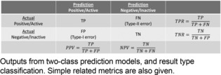
Confusion matrix.

While the raw counts of these four primary outcomes are informative, researchers often summarize a confusion matrix by a single, real‐valued metric, to decide on the quality of a model, to facilitate ranking of methods or datasets, and so forth. Two common, and potentially most intuitive, metrics are the true positive rate (TPR) and accuracy (ACC) metrics:

$${\displaystyle TPR=\frac{TP}{TP+FN}ACC=\frac{TP+TN}{TP+FP+TN+FN}.}$$

The former gauges how well positive instances were in fact classified by the model, and the latter gauges how well both positive and negatives instances are jointly classified. Hit finding teams may refer to the TPR when they wish to forecast the virtual screen of a large chemical library, and hit‐to‐lead and lead optimization teams might refer to ACC when considering the selectivity of a molecule, that is, the molecule's character to only interact with the targets intended by the molecule development team.

Studies that have executed prospective experimental validation of computationally predicted molecular properties often report low to medium success rates despite moderate to high model metric performance.4, 5, 6 While it is true that our understanding of the exact molecular underpinnings of processes is a continually evolving process and therefore we cannot build a perfect discriminant (model) of a phenomenon, a more fundamental problem exists in the metrics we often use to evaluate our results. In fact, metrics such as TPR and ACC often overestimate the “true” model performance. Action based on the misleading metrics incurs a risk to a project which can lead to misfortune, typically as a result of overconfidence in the discriminator computed.

In the remainder of this article, we illustrate the concerns around metrics such as TPR and ACC by shifting analysis away from single‐point numeric estimates to metric value surfaces (heatmaps) and considering some statistical properties of the metrics. While some previous attempts to objectify metrics exist,7, 8, 9, 10, 11, 12, 13, 14, 15, 16 this article is, to the best of our knowledge, the first to generically assess metric surfaces and their interplay with data balance. Further, we also propose a method to quantitatively cross‐compare metrics, and examine a practical case study in chemogenomic virtual screening.

2. Visual Cues Signaling Caution in Metric Interpretation

From the confusion matrix, many metrics are possible. In addition to the TPR and ACC introduced earlier, here we consider the Balanced Accuracy (BA), Positive Predictive Value (PPV), F‐measure and its derivative F1‐score (F1), True Negative Rate (TNR), and the Matthews Correlation Coefficient (MCC). These are defined mathematically as follows:

$${\displaystyle PPV=\frac{TP}{TP+FP}TNR=\frac{TN}{TN+FP}BA=\frac{TPR+TNR}{2}}$$

$${\displaystyle F1=\frac{2{}^{*}\left(PPV{}^{*}TPR\right)}{PPV+TPR}MCC=\frac{TP{}^{*}TN-FP{}^{*}FN}{\sqrt{(TP+FP)(TP+FN)(TN+FP)(TN+FN)}}.}$$

One fact we can immediately note from these definitions is how many types of results from the confusion matrix are included in each metric. TPR, TNR, and PPV include two types of results, and BA and F1 include three types of results. MCC and ACC include all four result types in their formulations, though only MCC includes both type‐I error and type‐II error in its numerator, and in a multiplicative manner. The range of values for the metrics are [−1,1] for the MCC, and [0,1] for all others.

Let us consider a simple example of two prediction experiments, and the resulting metric values for MCC and ACC. In the first experiment, we have TP=1000, TN=2100, FP=150, FN=650. We might consider this to be a rather successful prediction. The resulting ACC is 0.80 and resulting MCC is 0.58. Immediately, we notice that the MCC penalizes the type‐I and type‐II errors more than the ACC metric.

In the second experiment, let us assume that there were fewer positives in the dataset, and that TP=500, with TN, FP, and FN the same as above. We might also consider this to be successful based on the low false discovery rate (FPR), and when we evaluate the experiment by ACC the value is 0.76.

This is where we have deceived ourselves. Despite the high value of ACC, a re‐examination of the data would reveal that we made more type‐II errors than we correctly detected the positives. While the metric difference in the experiments for ACC was only 0.04, the latter experiment's MCC is 0.44, a metric difference of 0.14. We come to understand that the MCC is a more challenging metric to score high on, and that over‐expectations can be easily borne when using the ACC without considering the background data.

The additional issue we must be aware of is the ratio of data between the two classes. In many machine learning scenarios, equal numbers of positive and negative instances are used for model calculation and evaluation. However, in molecular informatics, this is a skewing of reality. For example, in experimentally‐based drug discovery and chemical biology, hit molecules are typically found at rates of 1 %.17,18 Even in less extreme examples where 10 %–25 % of the data belongs to the ‘positive’ (hit) class, metrics such as ACC can yield high values even if the model predicts everything as a negative (see below).

We can enhance our understanding of each metric's implications by considering the entire space of values it can take as a consequence of all possible type‐I and type‐II error rates, or alternatively and perhaps more intuitively, as a consequence of all possible TPRs and TNRs. As noted above, these rates are impacted by the ratio of data classes, and so should also be a factor in our interpretations.

We begin by visualizing the MCC and considering the impact of data ratio (Figure 2, left). We immediately note that having either high TPR or TNR is not a sufficient condition for high MCC. Extreme optimization on either positives or negatives can yield MCC values close to 0. Rather, both error rates must be low in order to achieve a high MCC. The situation in practical, imbalanced data is even more extreme (Figure 2, right); the region of the MCC surface which is at or above 0.6 is considerably reduced compared to the surface for balanced data.

Figure 2.

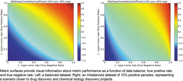
Metric landscape for MCC, balanced dataset versus imbalanced dataset.

When we consider the same pair of data ratio conditions but evaluate using ACC as shown in Figure 3, it becomes clear to us why ACC can trigger high expectations. Though extreme optimization on one class yields MCC values of 0, it yields ACC values of 0.5 in balanced datasets. Even worse, in hit and lead discovery applications with discovery rates of 10 % or less, a model can achieve a suggestively strong ACC of 0.8 or higher without even predicting a positive/active entity.

Figure 3.

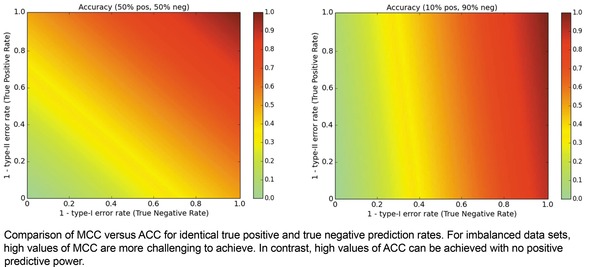
Metric landscape for ACC, balanced dataset versus imbalanced dataset.

As an additional way of analyzing the metrics, we might consider the distribution of values within the metric spaces shown in Figure 2 and Figure 3. This would yield a probability distribution function (assuming a small tolerance or bandwidth parameter), and we could compute the corresponding cumulative distribution function. Instead, let us consider the “inverse cumulative distribution function (iCDF)”, defined as the fraction of values in the metric space that are greater than or equal to a given metric value threshold. Our motivation for this is that we might ask, what is the probability of getting at least the value X for a particular metric? We can sample the performance matrix for the fraction of values that are at least a given value, and taken over the value domain of the metric, this yields a continuous plot and subsequent visual interpretation of the odds of obtaining a particular value or better of a metric. The resulting mirror image of a classic cumulative distribution function suggests the prefix “inverse”. Just as with the metric space visualization, the iCDF inherently depends on the class ratio.

The iCDF analogs of Figures 2 and 3 are shown in Figure 4. It confirms that the probabilities of obtaining metric values of 0.6 or 0.8 are many fold higher for ACC than for MCC, regardless of data ratio. The iCDF curves reinforce why misfortune may occur when basing decisions on model ACC values; the probability of achieving an ACC of 0.8 actually increases with a trend toward an imbalanced dataset. In contrast, one can feel more confident in a model that achieves MCC of 0.8, for the probability of such is rather low as an effect of its formulation.

Figure 4.

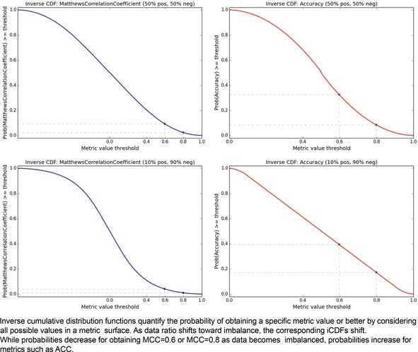
Metric iCDFs. Matthews Correlation Coefficient (left) versus Accuracy (right). Balanced datasets (above) versus imbalanced datasets (below).

Herein we have assumed that the prior probability of obtaining any particular value in the metric surface space is uniform. Yet in practical applications, this assumption will not hold, and priors will be influenced by datasets. Therefore, we can argue that the iCDFs given in Figure 4, notably for MCC, are optimistic estimates, and in reality, the gap between MCC and AUC iCDFs may in fact be even larger in practice.

The surfaces of the ACC, TNR, BA, F1, PPV, and MCC metrics are placed together in Figure 6 for a balanced ratio of data. For balanced data, we see that the F1 score also penalizes a high type‐II error rate and yields a metric value close to 0. This is a consequence of using the PPV and TPR in tandem. However, it is possible to over‐optimize on positives and score high with F1, so some caution is recommended. For balanced datasets, ACC and BA are synonymous.

Figure 6.

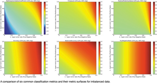
Multi‐metric surface comparison, Imbalanced data.

Figure 5.

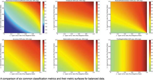
Multi‐metric surface comparison, Balanced data.

Turning to imbalanced datasets dominated by negatives/inactives (Figure 6), we see the rough correlation between the ACC and TNR surfaces, which reiterates the caution involved in using ACC. A predictor yielding an ACC of 0.9 on a strongly imbalanced dataset might potentially be a predictor of negatives and otherwise little more than chance. The BA metric is unchanged with respect to the data ratios. The clearest effect as a function of data ratio is on the F1 and PPV metrics. Much like MCC, the probabilities of obtaining higher F1 and PPV scores are strongly diminished when data is imbalanced, so models with high values under these conditions could be construed to be legitimately predictive in prospective applications.

Here as well, it is helpful to consider the iCDFs of the metrics. In Figure 7, an overlay of the iCDFs of the six metrics is shown, with separate views for balanced and imbalanced data. For balanced data, it is clearly more challenging to achieve a MCC value of 0.6 compared to other metrics. When data is imbalanced, ACC, BA, and TNR have higher odds of achieving 0.6 or 0.8 than F1, MCC, or PPV, and thus the former three statistics must be used with caution, particularly if the statistics will be a part of selecting models that will guide prospective applications.

Figure 7.

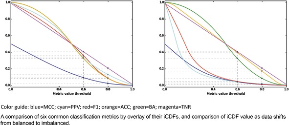
iCDFs of metrics, for balanced (left) and imbalanced (right) datasets.

Figures 5 and 6 demonstrate the clear shift in metric surfaces as a result of data imbalance, and Figure 7 objectifies the metric surfaces by iCDF analysis. An expanded analysis is still further possible by continuously varying the positive‐negative data ratio and connecting the per‐ratio snapshots. In the supplementary data, the interested reader can find animations of the shift in metric surface and iCDF. What do we learn from such animations? They provide us a better understanding of the dependence of a metric on the data ratio, and we gain skill in interpreting the significance of a given two‐class modeling experiment. Also, these animations expand our perspective for preparing prospective study design, by selecting metrics appropriate to the study context (vide supra).

We additionally provide pseudocode for the reader to develop visualizations of new metric approaches based on a confusion matrix. Code using the python programming language style, the NumPy matrix library,19 and the Matplotlib visualization library20 is given. First, the underlying surface matrices must be computed as follows.

Listing 1 – Code for Surface Matrix

“metric” is a calculable function using the arguments TP, TN, FP, and FN. “nPos” and “nNeg” refer to the numbers of positives and negatives representing the data.

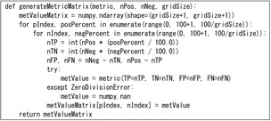
In the scheme in Listing 1, it is recommended to enforce that the “gridSize” parameter will be a value that evenly divides 100. The parameter will control the granularity of visualization and amount of memory required to compute the metric matrices.

Second, the matrix generated is to be visualized. Using the matplotlib library, this is relatively trivial. We add code to handle the case where a metric cannot be computed in extreme cases such as all examples predicted into the same class. This was handled in Listing 1 by the try‐except clause for errors caused by division by zero.

Listing 2 – Code for Metric Matrix Visualization

“fig” is a matplotlib Figure object, and “axes” is a matplotlib Axes object whose parent is “fig”. The “mat” is generated by Listing 1. A matplotlib Colormap object “cmap” is provided to standardize the same color scheme across the metrics. Additional arguments stored in the “args” key‐value mapping control the final visualization rendered.

3. Metrics and the Receiver Operating Characteristic Curve

Another highly common method for assessing the performance of a modeling method is the generation of a receiver operating characteristic (ROC) curve, and the area under such a generated curve. ROC curves are most commonly built by using cross‐validation techniques that perform multiple rounds of dataset splitting, such that each round of prediction values can be included in a more comprehensive list of thresholds which will yield a per‐threshold pair of values for TPR and Type‐I error rate (the TPR and Type‐I error will be computed using the entire collection of predictions spanning all rounds of dataset splitting). Threshold values could be, to name only a few, distances from hyperplanes when using the SVM algorithm21 or the percentage of tree votes when using a random forest algorithm.22 A plot of all TPR and Type‐I error rates using all thresholds then results in a curve indicating the tradeoff between optimizing on the two metrics. If a threshold can be found such that it can discriminate all or most of the positives from the negatives, then it will result in an area under the ROC curve close to 1. For further explanation, see the literature on ROC and extensions to ROC.15

To analyze the AUC in the same metric surface framework, one modification is needed. In the case of ACC, MCC, and similar metrics, fixed counts of positives and negatives (and hence their ratio) completely determine the resulting surface (because we can iterate the grid of TPR and TNR independent of an actual model). However, in the case of AUC, a range of thresholds obtained from cross‐validated modeling and prediction is required for metric calculation. Therefore, instead of generating a grid of TPR/TNR, we must generate a grid of positive and negative dataset sizes, and execute cross‐validation with accompanying AUC calculation at each point. Repeated executions and computation of average AUC minimize outlier values that may occur.

We execute two AUC calculation and surface analysis experiments. In the first, we use artificial stochastic classifier functions (random selectors based on underlying distributions) as surrogates of models computed from real data. In the second, we apply the SVM algorithm to large‐scale public GPCR GLASS23 and Kinase SARfari24 ligand‐target bioactivity datasets, where the active/inactive thresholds are set to 100nM/1‐10uM, and intermediate strength interactions are discarded (for further data processing details, see Reker et al.25); the human‐based, filtered datasets contains 49815 actives (71 %) versus 20145 inactives for GLASS, and 19231 actives (48 %) versus 20475 inactives for SARfari, with compounds and proteins respectively represented by their MACCS key and dipeptide frequency representations. Experiments for the artificial classifiers use 200 iterations for AUC averaging, and experiments for GPCR/kinase bioactivity classifications compute average AUC over 20 iterations of 3‐fold cross‐validation. In addition to AUC calculation, a subset of data is held out for external prediction when using the real datasets. A diagram of execution flow is provided as supplementary data.

For the artificial classifiers, we find that average AUCs are not influenced by the sizes of positives and negatives (see supplementary data). Rather, the surfaces are dominated by the parameters of the stochastic selection process (e. g., mean and standard deviation of a random Gaussian variable).

In contrast, however, we find that AUC values in the real dataset are influenced by positive/negative size, and they are simultaneously influenced by model parameters (e. g., tolerance factor “C” and radius parameter γ for SVMs using radial basis function kernels). Importantly, we find that the AUC grows in proportion to the size of data available for cross‐validation, and that it is possible to obtain similar AUC values for datasets with opposite positive/negative ratios. In extreme cases with many data in one class, we return to an argument similar to ACC on a dominantly negative dataset (Figures 3 and 6); it may be relatively trivial to build even a linear classifier that separate the dominant class from the infrequent class. Such results again suggest that careful interpretation of modeling performance is required, and that comparison of AUC values on datasets of differing source or size requires caution.

In addition to cross‐validated AUC, it is possible to consider cross‐validated MCC or F1 score. In the cases of the latter metrics, they require the pre‐specification of a threshold value which is compared against the raw output of the classifier, at which raw prediction results are discretized, and the metric is calculated from the resulting confusion matrix. We performed this additional analyses by setting the thresholds for MCC and F1 to the obvious value of 0, which means to simply use the sign of the raw output corresponding to which side of the SVM hyperplane an example was classified on.

For both the GLASS and SARfari datasets, we computed a single model using a fixed ratio of subsampled data at a given grid point, and evaluated external prediction on the remaining portion. Experiments were done using ratios of 0.33, 0.5, and 0.7, respectively reflecting scenarios where a majority of data was used for CV, where data was evenly split for CV and external prediction, and where data was reduced such that predictive performance on a much larger external set could be evaluated. As an example, at an external data ratio of 50 %, where the imbalanced grid point contained 234 active and 1234 inactive ligand‐target pairs subsampled from the larger database, 117 actives and 617 inactives formed the external prediction set, and the remaining data (of equal size) was used for 3‐fold cross‐validation. Hence each round of 3‐fold CV could build models using 117*(2/3)=78 actives and 411 inactives, and predict on the remaining 206 as well as obtain their raw values to use as thresholds in ROC curve generation. Models used to evaluate the external set would be built on the full 117 actives and 617 inactives. Where the external ratio was 0.7, for example, the model building was on 70 actives and 370 actives, with external prediction on 164 actives and 864 inactives.

In the upper half of Figure 8, the cross‐validated AUC and cross‐validated MCC/F1 are evaluated over the grid of data sizes for the SVM with an RBF kernel, where the external split ratio was 0.5. The trend of AUC to grow with imbalance is clear, as well as a further increase in average AUC as the numbers of positives and negatives exponentially grow. The MCC also grows as the data available for cross‐validation grows, but unlike AUC, MCC performance at extremes is 0, and it is not until a moderate number of samples from both classes are available that the MCC climbs to a positive number. Interestingly, we see a dichotomy in F1‐CV metric surface behavior, where F1 is potentially over‐estimated for models with disproportionate numbers of actives, and like MCC, at or close to 0 for dominantly inactive datasets. Like MCC and AUC, F1 performance is appropriately high when both larger numbers of actives and inactives are included.

Figure 8.

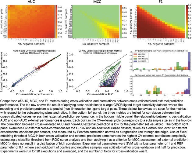
Cross‐validation, external prediction, metrics, and their cross‐correlations.

Next, we considered how well each metric performed in cross‐validation settings versus external prediction settings. The results, shown in the bottom‐left panel of Figure 8, suggest that cross‐validated training performance accurately estimates external prediction performance, though admittedly, experience suggests that external performances are often lower than training performances, which was observed for other parameter sets tested. It may be the case that repeated trials nullified the effect of any one poor external prediction, and that the random sampling selected ligand‐target pairs from similar distributions.

In practical situations of prospective prediction, a single threshold must be applied to generate the list of prospective validations to execute, and so while AUC is computable in a retrospective setting, it is not transferrable to prospective settings. To address this, we checked the correlation between cross‐validated AUC and MCC at the baseline threshold of 0. No correlation was observed, as shown in the bottom‐middle panel of Figure 8. This was concordant with another recent study examining correlation on artificially generated data.16

We further considered, however, that it is possible to select a single point on the ROC curve which contains a permissible false discovery rate, and use that threshold as the criteria for MCC or F1 evaluation. In other words, if we determine by cross‐validation the threshold that maximized the true positive rate up to the extent we tolerate error, then that could serve as the threshold in our prospective application. Solving the threshold value for a tolerable false discovery rate of 10 %, we then applied the F1 and MCC metrics with such threshold, and again examined the relationship between cross‐validated AUC and external prediction. As shown in Figure 8 (bottom‐middle), this correlation was also weak, though the thresholded MCC slightly better correlated to AUC than default‐thresholded MCC. Hence, generating expectations of success based on multi‐threshold AUC may fail to correlate with single‐threshold ACC/MCC/etc in post‐experiment, prospective performance analyses.

Finally, at a larger scale, we asked what the correlation of cross‐validated AUC would be with external AUC, of CV–MCC with external MCC, of CV‐AUC with external MCC, and of CV‐AUC with thresholded MCC, by iterating tests over a small parameter grid and across both datasets (4 SVM parameter sets * 3 external ratios * 2 datasets), and asking what the correlation of these pairs are at each grid point. That is, correlation metrics were used to assess the fit between a pair of metrics using all points of the positive/negative subsampling grid and resulting metrics. Correlations were computed not only by Pearson correlation but also by alternatively forcing the regression line to pass through the origin, as proposed previously by Golbraikh and Tropsha.26

As can be expected, the distribution of Pearson correlations were higher than the origin‐fitting correlations, as shown in the bottom‐right panel of Figure 8. Importantly, we see that when basing decisions on the correlations obtained in the more stringent correlation fit, the AUC‐AUC and MCC–MCC metric pairs emerge with the strongest correlation. Yet, as argued above, using the entire range of raw prediction values for the external set to generate an AUC is only applicable in retrospective scenarios. Therefore by elimination, it would appear that cross‐validated MCC is the most reliable method to estimate prospective performance on a similar‐sized external prediction.

4. Conclusion and Future Outlook

Using the tandem of metric surfaces and iCDFs, we can improve our understanding of the consequences of selecting a particular metric in order to evaluate predictive performance of two‐class discriminants. We find that TPR, TNR, or ACC alone run the risk of deception; the physicist Richard Feynman once remarked that “… you must not fool yourself, and you are the easiest person to fool.”

Metrics such as MCC or F1 score provide more realistic estimates of real‐world model performance, and in imbalanced datasets skewed toward negative data, PPV might be indicative of expected discovery rates. The practical chemogenomic virtual screening experiments showed a lack of correlation between MCC and F1, and between AUC and MCC. Taken together, the best advice we can suggest is to take a multi‐metric view of molecular modeling, and place the model task context at the center of metric interpretation.

Though the MCC might appear to be the “best” metric available by including all four types of results from the confusion matrix, several prediction problems do not lend themselves to use of the metric. For example, evaluating prediction of DNA sequence variants from next‐generation sequencing frequently leads to focus on TP, FP, and FN results; though it is technically possible to count the total number of nucleotides that were correctly not called variants, this number would be cosmological compared to the other three raw counts in the confusion matrix, and it therefore stands to reason to use TPR, PPV, or their combination in the form of the F1 score or more general F‐measure.

What can the scientific community do in order to close the gap between computed prediction expectation and experimental validation success rates? The thorough consideration of metrics prior to the execution of a study is certainly a crucial element. If a new classification evaluation metric is suggested, then its surface should be visualized and its iCDF should be compared to others such as the ones given in this report. A high probability of obtaining a particular metric value as assessed by iCDF should be cross‐referenced with its surface visualization to determine if there is a risk or element of deception resulting from many possible ways to arrive at the metric value in question (i. e., there are many ways to achieve ACC of at least 0.6 in inbalanced data). Computational experiments may consider the philosophy discussed herein to perform repeated executions of a model‐predict experiment such that less than half of the data per class is subsampled for model selection with the majority remainder used for prediction. Recent modeling methods have shown that often only a fraction of a dataset is sufficient to build a predictive model.25,27,28 As in the prior studies, if distribution of prediction performances can be shown to be normally distributed by the Kolmogorov‐Smirnov test, we can consider using such a fact to forecast the chances of success in a true prospective experiment.

Finally, we remark that the discussion here is contained to two‐class prediction, while some molecular informatics modeling tasks may need to classify an instance amongst three or more classes (i. e., protein sequence secondary structure prediction, or prediction of ligands as strong/weak/intermediate). In these cases, the visualization might be expanded to a 3D voxel representation, but for four or more classes, views of subspaces of the metric space are required. A well‐known metric for the multi‐class discriminant is Cohen's Kappa Coefficient.29 The iCDF concept introduced herein could be applied by shifting from a matrix (2‐tensor) to a generalized tensor yielded by the computation of all per‐class prediction rates. The iCDF would be continue to be influenced by the data ratio, where in the generalized case a partitioning of data class ratios must be provided.

Supplementary Data

Animations of the relationship between data ratio and metric surface, and between data ratio and iCDF are available online. A fully executable standalone tool for surface generation is also provided. Stochastic selection and practical chemogenomic model AUC results can also be retrieved. Results analogous to Figure 8 for the Kinase SARfari dataset are provided, and observations of correlations between CV‐AUC and MCC/MCC(t)/F1 for many parameter sets are made available.

Conflict of Interest

None declared.

Biographical Information

J. B. Brown obtained dual B.S. degrees in Computer Science and Mathematics from the University of Evansville (Indiana, USA). Following undergraduate studies, he worked at the NIH clinical center, contributing to a computational platform for automated diagnostic radiology image analysis and therapy decision support. In 2004, he was awarded a full scholarship from the Japanese government, and began his garduate studies at Kyoto University, completing a Ph.D. in bio‐ and chemo‐informatics in 2010. After a post‐doctoral appointment in pharmaceutical sciences, he was promoted to an assistant professor at the Kyoto University Graduate School of Medicine in 2014. In 2015, he was awarded an independent (PI) Junior Associate Professor position within the same graduate school, and founded his Life Science Informatics Research Unit, a unit hybridizing clinical, chemical, and biological informatics.

Supporting information

As a service to our authors and readers, this journal provides supporting information supplied by the authors. Such materials are peer reviewed and may be re‐organized for online delivery, but are not copy‐edited or typeset. Technical support issues arising from supporting information (other than missing files) should be addressed to the authors.

Supplementary

Supplementary

Supplementary

Supplementary

Supplementary

Supplementary

Supplementary

Supplementary

Supplementary

Supplementary

Supplementary

Supplementary

Supplementary

Supplementary

J. B. Brown, Mol. Inf. 2018, 37, 1700127.

References

- 1. Schneider G., Nat. Rev. Drug Discovery 2010, 9, 273–276. [DOI] [PubMed] [Google Scholar]
- 2. Bajorath J., Barreca M. L., Bender A., Bryce R., Hutter M., Laggner C., Laughton C., Martin Y., Mitchell J., Padova A., et al., Future Med. Chem. 2011, 3, 909–21. [DOI] [PubMed] [Google Scholar]
- 3. Clark D. E., Expert Opin. Drug Discovery 2008, 3, 841–851. [DOI] [PubMed] [Google Scholar]
- 4. Ripphausen P., Nisius B., Peltason L., Bajorath J., J. Med. Chem. 2010, 53, 8461–8467. [DOI] [PubMed] [Google Scholar]
- 5. Ripphausen P., Nisius B., Bajorath J., Drug Discovery Dev. 2011, 16, 372–376. [DOI] [PubMed] [Google Scholar]
- 6. Ripphausen P., Stumpfe D., Bajorath J., Future Med. Chem. 2012, 4, 603–613. [DOI] [PubMed] [Google Scholar]
- 7. Chu C. W., Holliday J. D., Willett P., Bioorganic Med. Chem. 2012, 20, 5366–5371. [DOI] [PubMed] [Google Scholar]
- 8. Chu C.-W., Holliday J. D., Willett P., J. Chem. Inf. Model. 2009, 49, 155–161. [DOI] [PubMed] [Google Scholar]
- 9. Abdo A., Chen B., Mueller C., Salim N., Willett P., J. Chem. Inf. Model. 2010, 50, 1012–1020. [DOI] [PubMed] [Google Scholar]
- 10. Chen B., Harrison R. F., Papadatos G., Willett P., Wood D. J., Lewell X. Q., Greenidge P., Stiefl N., J. Comput.-Aided Mol. Des. 2007, 21, 53–62. [DOI] [PubMed] [Google Scholar]
- 11. Jurman G., Riccadonna S., Furlanello C., PLoS One 2012, 7, e41882. [DOI] [PMC free article] [PubMed] [Google Scholar]
- 12. Lopes J. C. D., dos Santos F. M., Martins-José A., Augustyns K., Winter H. De, J. Cheminform. 2017, 9, 7. [DOI] [PMC free article] [PubMed] [Google Scholar]
- 13. Luo J., Schumacher M., Scherer A., Sanoudou D., Megherbi D., Davison T., Shi T., Tong W., Shi L., Hong H., et al., Pharmacogenomics J. 2010, 10, 278–291. [DOI] [PMC free article] [PubMed] [Google Scholar]
- 14. Baldi P., Nasr R., J. Chem. Inf. Model. 2010, 50, 1205–1222. [DOI] [PMC free article] [PubMed] [Google Scholar]
- 15. Swamidass S. J., Azencott C.-A., Daily K., Baldi P., Bioinformatics 2010, 26, 1348–1356. [DOI] [PMC free article] [PubMed] [Google Scholar]
- 16. Boughorbel S., Jarray F., El-Anbari M., PLoS One 2017, 12, e0177678. [DOI] [PMC free article] [PubMed] [Google Scholar]
- 17. Lopez-Sambrooks C., Shrimal S., Khodier C., Flaherty D. P., Rinis N., Charest J. C., Gao N., Zhao P., Wells L., Lewis T. A., et al., Nat. Chem. Biol. 2016, 12, 1023–1030. [DOI] [PMC free article] [PubMed] [Google Scholar]
- 18. Severyn B., Nguyen T., Altman M. D., Li L., Nagashima K., Naumov G. N., Sathyanarayanan S., Cook E., Morris E., Ferrer M., et al., J. Biomol. Screening 2016, 21, 989–997. [DOI] [PubMed] [Google Scholar]
- 19.S. Van Der Walt, S. C. Colbert, G. Varoquaux, 2011, DOI 10.1109/MCSE.2011.37.
- 20. Hunter J. D., Comput. Sci. Eng. 2007, 9, 90–95. [Google Scholar]
- 21. Cortes C., Vapnik V., Mach. Learn. 1995, 20, 273–297. [Google Scholar]
- 22. Breiman L., Mach. Learn. 2001, 45, 5–32. [Google Scholar]
- 23. Chan W. K. B., Zhang H., Yang J., Brender J. R., Hur J., Özgür A., Zhang Y., Bioinformatics 2015, 31, btv302-. [DOI] [PMC free article] [PubMed] [Google Scholar]
- 24. Bento A. P., Gaulton A., Hersey A., Bellis L. J., Chambers J., Davies M., Krüger F. A., Light Y., Mak L., McGlinchey S., et al., Nucleic Acids Res. 2014, 42, D1083–90. [DOI] [PMC free article] [PubMed] [Google Scholar]
- 25. Reker D., Schneider P., Schneider G., Brown J., Future Med. Chem. 2017, 9, 381–402. [DOI] [PubMed] [Google Scholar]
- 26. Golbraikh A., Tropsha A., J. Mol. Graph. Model. 2002, 20, 269–76. [DOI] [PubMed] [Google Scholar]
- 27. Lang T., Flachsenberg F., Von Luxburg U., Rarey M., J. Chem. Inf. Model. 2016, 56, 12–20. [DOI] [PubMed] [Google Scholar]
- 28. Rakers C., Reker D., Brown J. B., J. Comput. Aided Chem. 2017, 8, 124–142. [Google Scholar]
- 29. Cohen J., Educ. Psychol. Meas. 1960, 20, 37–46. [Google Scholar]
Associated Data
This section collects any data citations, data availability statements, or supplementary materials included in this article.
Supplementary Materials