Cell Membrane Tracking in Living Brain Tissue using Differential Interference Contrast Microscopy

Abstract

Differential Interference Contrast (DIC) microscopy is widely used for observing unstained biological samples that are otherwise optically transparent. Combining this optical technique with machine vision could enable the automation of many life science experiments; however, identifying relevant features under DIC is challenging. In particular, precise tracking of cell boundaries in a thick (> 100µm) slice of tissue has not previously been accomplished. We present a novel deconvolution algorithm that achieves state-of-the-art performance at identifying and tracking these membrane locations. Our proposed algorithm is formulated as a regularized least-squares optimization that incorporates a filtering mechanism to handle organic tissue interference and a robust edge-sparsity regularizer that integrates dynamic edge-tracking capabilities. As a secondary contribution, this paper also describes new community infrastructure in the form of a MATLAB toolbox for accurately simulating DIC microscopy images of in vitro brain slices. Building on existing DIC optics modeling, our simulation framework additionally contributes an accurate representation of interference from organic tissue, neuronal cell-shapes, and tissue motion due to the action of the pipette. This simulator allows us to better understand the image statistics (to improve algorithms), as well as quantitatively test cell segmentation and tracking algorithms in scenarios where ground truth data is fully known.

I. Introduction

LIVE cell imaging allows the monitoring of complex biophysical phenomena as they happen in real time, which is beneficial in studying biological functions, observing drug action, or monitoring disease progression. For these experiments, tissue from an organ such as brain, heart, or liver is sliced and imaged while it is still alive [1]–[4]. Fluorescence microscopy is often used for live cell imaging but is not always practical because it requires the use of dyes or genetic engineering techniques to introduce fluorophores into the sample. Instead, it is often desirable to image unlabeled, otherwise optically transparent samples. This is often done using a phase contrast-enhancing technique such as differential interference contrast (DIC) microscopy.

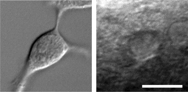
Using machine vision to automatically segment individual cells under DIC optics in real time would be highly useful for microscopy automation of life science experiments. However, precise cell segmentation is challenging and the vast majority of existing algorithms are not directly applicable to segmentation under DIC in tissue. General purpose segmentation algorithms in the computer vision literature typically assume statistical homogeneity within (or outside) a segmentation region that would be lost under contrast-enhancing optical approaches such as DIC. While it is possible that these algorithms could be applied after application-specific pre-processing [5], [6], these existing approaches are not directly applicable to the target application without being combined with deconvolution. There are additionally a number of specific cell segmentation and tracking methods that [7]–[12] are also not directly applicable to cell segmentation under DIC in tissue. For example, algorithms proposed in the Cell Tracking Challenge [13], [14] are developed on the CTC dataset that consists only of microscopy imagery of cultured cells (rather than tissue slices) that had minimal organic tissue interference (Fig. 1). These cell-tracking methods (1) often assume simple noise statistics, (2) target gross cell location tracking for mechanobiology tasks (e.g., studies on cell migration, morphology) rather than precise membrane localization, and (3) are designed to be run offline rather than in real-time [15].

Fig. 1.

Images obtained with DIC microscopy (40× magnification). Left: cultured human embryonic kidney (HEK293) cell. Right: neuron in mouse brain tissue (400 um thickness). The image on the right has high levels of imaging noise due to light scatter and interference due to organic material in surrounding tissue. Scale bar 10 µm.

We present the first cell segmentation and boundary tracking algorithm for DIC imagery of tissue slices. While our broad approach may generalize to other tasks, we focus here on one experiment type: patch-clamp recording in brain tissue. In this experimental paradigm, brain tissue is sliced into 100–400µm thick sections, each containing thousands of neurons embedded in a dense biological milieu. The slice is imaged with a microscope and glass probe is inserted into the tissue to sample the electrical activity of individual cells [16], [17]. While manual patch clamp electrophysiology is considered to be the gold-standard for high-fidelity single-cell analysis, the challenge and labor intensity of the process makes it extremely advantageous to automate. Recent work has demonstrated the possibility of automating the patch clamp process by using a motorized robotic actuator to maneuver the probe to the target cell [18], [19]; for this purpose, real-time tracking of the target cell boundary is essential. This application presents several challenges that make cell membrane localization very difficult: (1) heavy interference from the presence of organic tissue around the target cell, (2) low SNR due to scattering of light characteristic of thick tissue samples, and (3) cell motion induced by the glass probe.

Extending the framework provided by [20], our proposed algorithm is formulated as a regularized least-squares optimization that incorporates a filtering mechanism to handle organic tissue interference and a robust edge-sparsity regularizer that integrates dynamic edge-tracking capabilities. We specifically note that the proposed algorithm is performing a deconvolution of the complex effects of DIC imaging integrated into a segmentation process and is not a direct segmentation of raw DIC images. Toward this end, our focus is specifically on cell boundary tracking instead of more typical deconvolution metrics such as least-square image reconstruction. Ancillary to our main contribution, this paper also describes new community infrastructure in the form of a MATLAB toolbox for accurately simulating DIC microscopy images of in vitro brain slices. Building on existing DIC optics modeling, our simulation framework additionally contributes an accurate representation of interference from organic tissue, neuronal cell-shapes, and tissue motion due to the action of the pipette. This simulator allows us to better understand the image statistics to improve algorithms, as well as quantitatively test cell segmentation and tracking algorithms in scenarios where ground truth data is fully known. The simulation toolbox is freely available under GNU GPL at http://siplab.gatech.edu.

II. Background

A. DIC microscopy

DIC microscopy enhances the contrast of an image by exploiting the fact that differences in the tissue will have different optical transmission properties that can be measured through the principle of interferometry. Specifically, the signal that we aim to reconstruct is known as the optical path length (OPL) signal image, which is proportional to the the underlying phase-shift. The OPL is defined as the product of refractive index and thickness distributions of the object relative to the surrounding medium [20], [21]. This OPL signal shall be denoted as x_k ∈ ℝ^N (a vectorized form of the $\sqrt{N}\times \sqrt{N}$ OPL image’s intensity values), and indexed in time by subscript k. DIC microscopy amplifies differences between the cell’s refractive index and its environment to enhance visibility of the cell, highlighting edge differentials and giving the appearance of 3D relief. This effect may be idealized as a convolution between the optics’ point spread function and the OPL, and denoted as Dx_k, where D ∈ ℝ^{N × N} is a matrix that captures the 2D convolution against a kernel d ∈ ℝ^{K × K}.

While more sophisticated DIC imaging models (c.f., [22]) exist, for simplicity we use a kernel d corresponding to an idealized DIC model proposed by Li and Kanade [20] which is a steerable first-derivative of Gaussian kernel:

$$d(x,y)\propto -x\text{ cos}(\theta )·e^{-\frac{x^2+y^2}{{\sigma }_d^2}}-y\text{ sin}(\theta )·e^{-\frac{x^2+y^2}{{\sigma }_d^2}},$$ (1)

where σ_d refers to the Gaussian spread and θ_d refers to a steerable shear angle. This model assumes an idealized effective point spread function (EPSF), where the condenser lens is infinite-sized and the objective is infinitely small (with respect to the wavelength). This model also ignores any phase wrapping phenomenon by assuming that the specimen is thin enough or the OPL varies slowly enough such that it behaves in the linear region of the phase difference function [22]. In practice, d(x, y) is discretized as d with a proportionality constant of 1, and with x and y each taking the discrete domain $\{-\frac{K-1}{2},-\frac{K-3}{2},\dots ,\frac{K-3}{2},\frac{K-1}{2}\}$.

B. Deconvolution Algorithms

DIC cell segmentation algorithms fall broadly into three categories: direct, machine-learned, or deconvolution (or phase-reconstruction) algorithms. Direct algorithms apply standard image processing operations such as low-pass filtering, thresholding, and morphological shape operations [5], [6], [23] but are not robust and work only on very low-noise/interference imagery. Machine-learned algorithms perform statistical inference learned from a large number of cell-specific training images (e.g., deep convolutional networks [24] or Bayesian classifiers [25]). Such algorithms have been shown to perform coarse segmentation surprisingly well in challenging scenarios (e.g., cells with complicated internal structures with low-noise/interference) for applications like cell-lineage tracking or cell-counting, yet they appear to lack precision for accurate cell-boundary localization. Deconvolution algorithms [22], [26]–[29] may be defined as a reconstructive process which estimates the OPL (or phase-shift image) that has been convolved by the DIC microscopes optical point spread function. Early work involved closed-form reconstructive methods such as deconvolution by Wiener filtering [22] or the Hilbert transform [27], [29] which were not robust against noise. Other work involved DIC deconvolution by constraining the support of deconvolution along a single line along the shear axis [28]. While computationally quick, this made the reconstruction prone to discontinuities between lines (especially in high-noise/interference images), resulting in significant streaking artifacts which corrupt the cell boundary estimates. Deconvolution (in 2D) was proposed in [26] by assuming some linear approximation to the point spread function optical model, yet this formulation lacked regularization, thus making the problem ill-posed and also highly susceptible to noise.

Recent developments in fast and robust ℓ₁ (i.e., ‖·‖₁) reconstruction approximations motivated Li and Kanade to develop a mixed-norm pre-conditioning approach [20] that exploited sparsity and smoothness in the OPL image using ℓ₁-norm and total variation (TV) norm (i.e., ‖·‖_TV) regularizers:

$${\hat{\mathit{x}}}_k=\text{arg}\underset{\mathit{x}\ge \mathbf{0}}{\text{min}}\frac{1}{2}{\Vert {\mathit{y}}_k-\mathit{\text{Dx}}\Vert }_2^2+\beta {\Vert \mathit{x}\Vert }_1+\gamma {\Vert \mathit{x}\Vert }_{\mathit{\text{TV}}},$$ (2)

where β, γ are sparsity and smoothness parameters that control the weight of pixel sparsity and edge-sparsity against reconstruction fidelity respectively. The same paper proposed an alternative approach that replaced the TV norm by a Laplacian Tikhonov term to make it more computationally efficient, but placed less emphasis on smoothness:

$${\hat{\mathit{x}}}_k=\text{arg}\underset{\mathit{x}\ge \mathbf{0}}{\text{min}}\frac{1}{2}{\Vert {\mathit{y}}_k-\mathit{\text{Dx}}\Vert }_2^2+\beta {\Vert \mathbf{\Lambda }\mathit{x}\Vert }_1+\gamma {\Vert \mathit{\text{Lx}}\Vert }_2^2,$$ (3)

where Λ is a positive weighting diagonal matrix (which may be optionally applied to further encourage pixel-sparsity), and L is a matrix that applies a 2D convolution of a Laplacian filter against the image.

A recent deconvolution algorithm intended to facilitate cell segmentation [30] advanced the work in [20] by reducing the computational complexity as well as introducing a dynamical prior (exploiting temporal structure) and a re-weighting process that improves reconstruction accuracy. The core algorithm can be summarized by two steps, an optimization step and a reweighting step as follows:

$${\hat{\mathit{x}}}_k^{(t)}=\text{arg}\underset{\mathit{x}\ge \mathbf{0}}{\text{min}}\frac{1}{2}{\Vert {\mathit{y}}_k-\mathit{\text{Dx}}\Vert }_2^2+\beta {\Vert {\mathbf{\Lambda }}^{(t)}\mathit{x}\Vert }_1+\gamma {\mathit{x}}^{\top }\mathit{\text{Jx}}+\kappa {(\mathit{x}-{\hat{\mathit{x}}}_{k-1})}^{\top }\sum (\mathit{x}-{\hat{\mathit{x}}}_{k-1}){\mathbf{\Lambda }}^{(t+1)}[\mathit{\text{ii}}]=\frac{1}{{\hat{\mathit{x}}}_k^{(t)}[i]+\eta },$$ (4)

where ⊤ refers to the transpose operator, Λ is a positive diagonal matrix defining the ℓ₁ weights, J is a Laplacian matrix defining similarity between spatial neighbors, Σ is a matrix defining the similarity between temporal pixel neighbors, t represents the algorithmic iteration index, κ is a parameter that controls the influence of the dynamical regularizer, and η is a small positive constant that prevents division by zero. These methods were effective at retrieving the OPL for noisy microscopy images with little interference. However, organic tissue interference surrounding the cell negatively affected the reconstruction (and subsequently segmentation), especially around the edges of the cell (later demonstrated in Section IV).

C. Reweighted ℓ₁ Algorithms

The reweighted ℓ₁ framework introduced by Candes et al. [31] was found to produce robust reconstructions because each signal element’s statistics were individually parameterized as opposed to having them globally parameterized by a single term (in the non-weighted ℓ₁ setup). Garrigues et al. [32] furthered this work using the Bayesian inference framework, and formulated it as a hierarchical probabilistic model, treating the signal elements as Laplacian random variables conditioned by the weights. Their key contribution was that the weights themselves could be treated as random variables with Gamma hyperpriors, and that solving the maximum a posteriori estimation using the expectation maximization (EM) approach admitted a closed form expectation-step for the weight update. Charles et al. applied this framework to design a robust dynamical ℓ₁ reweighing algorithm [33] by crafting how dynamical information should propagate through the distribution of the hyperprior. In essence, by reweighing of the ℓ₁ term using dynamics, second order statistics are propagated through time in a spirit similar to the Kalman filter. This method, though very effective for the tracking of sparsely distributed signals, could not be directly applied to our problem since our signal space (i.e., our DIC imagery) distribution was not adequately sparse (as will be later shown, in Section IV, by the inferiority of ℓ₁ methods).

The reweighted TV minimization was introduced in [31] as a regularization method (in compressive sensing), for recovering the Shepp-Logan phantom [34] from sparse Radon projections, demonstrating potential for application in bio-imagery. The method however has never been applied to cellular imagery, nor has it the capability to exploit dynamical information in temporal data.

D. Cell Simulator

Accurate cell simulators are a valuable tool for two reasons: they allow objective testing with known ground truth, and provide insights into generative models that facilitate algorithm development. Currently, the vast majority of existing cell simulator packages focus specifically on fluorescence microscopy [35]–[39] rather than DIC microscopy. While some simulators [36], [37] excelled at providing a large variety of tools for simulating various experimental scenarios and setups, most lacked simulation of synthetic cellular noise similar to that found in DIC microscopy images of brain slices (due to the presence of cellular tissue). Most simulators tend to target very specific types of cells [35], [36], [39] and there have been initial efforts to organize and share cellular information (e.g., spatial, shape distributions) into standardized formats across simulators [15], [16]. Despite this, no existing simulator currently generates synthetic DIC imaging of neurons such as those used in patch clamp experiments for brain slices. To facilitate algorithm design and evaluation on the important problem of automated patch clamping, we have built and released MATLAB toolbox for accurately simulating DIC microscopy images of in vitro brain slices (described in Appendix A and freely available under GNU GPL at http://siplab.gatech.edu).

III. Deconvolution Algorithm

The goal of the system is to provide automated visual tracking of the membrane of a user-selected target cell to guide a robotic patch clamping system. We will achieve these goals with an approach described by three general stages visualized by Fig. 2. The first stage uses standard computer vision tracking techniques to identify the general patch of interest containing the target cell on the current frame. The second stage implements dynamic deconvolution to recover a time-varying OPL image that can be used for segmentation. The novel contribution of this paper is a proposed deconvolution algorithm for this stage, and the details of this algorithm will be the focus of this section. We will also describe an extension of the basic proposed algorithm that retains good performance when the recording pipette overlaps with the cell by removing the pipette image and performing inpainting. The third stage is a segmentation on the output of the deconvolution, which is performed with simple thresholding.We point out that a simple segmentation strategy is sufficient after a robust deconvolution process.

Fig. 2.

The full required imaging system has three stages: patch tracking, deconvolution, and segmentation. In patch tracking, a user-defined template is provided for template matching and tracking spatial coordinates over time with a Kalman filter. In deconvolution (the main focus of this paper), the patch is deconvolved to infer the OPL approximation. In segmentation, a global threshold is applied (using Ostu’s method [45]) to yield a binary segmentation mask to determine the cell membrane location.

A. Preliminaries

The deconvolution and segmentation algorithms will be run on a limited image patch size (e.g., 64 × 64, as a trade-off between speed and resolution) that is found by tracking gross motion in the image. Specifically, template matching (via normalized cross-correlation) is performed on each frame using a user-selected patch (e.g., obtained via a mouse-click to associate coordinates of the image patch center with the targeted cell’s center). Patch-tracking robustness may be improved by running a standard Kalman filter on the positional coordinates of the found patch (i.e., tracking a two-dimensional state vector of the horizontal and vertical location of the patch center). To ensure efficacy with the correlation approach, a preprocessing stage of lighting bias elimination (i.e., uneven background substraction) is performed on each video frame¹ using quadratic least squares estimation (with a polynomial order of 2) as described in [20] and by Eq. (14). While tracking the detailed cell membrane locations is challenging, tracking the general location of the patch containing the target cell can be done with very high accuracy using this approach. Yet, more sophisticated and robust computer vision methods such as multi-cue visual tracking [40]–[43] can replace this basic correlation approach to improve on the patch-tracker’s performance. Specific implementation details to the template matching approach may be found in [44].

Following insight gained from developing the simulator in Appendix A, we assume that at each time step (indexed by k) the bias eliminated image has the following generative model:

$${\mathit{y}}_k={\mathit{\text{Dx}}}_k+{\mathit{n}}_k^{\mathit{\text{organic}}}+{\mathit{n}}_k^{\mathit{\text{sensor}}},$$

where y_k ∈ ℝ^N is the vectorized form of the microscopy image (e.g., 64 × 64 image patch), ${\mathit{n}}_k^{\mathit{\text{organic}}}\in {ℝ}^N$ is a noise component consisting of organic materials surrounding the cell and modeled by a non-white Gaussian distribution (i.e., non-flat frequency profile), and ${\mathit{n}}_k^{\mathit{\text{sensor}}}\in {ℝ}^N$ consists of 2 distinct additive noise elements: thermal noise modeled as a white-Gaussian distribution and photon noise modeled as a Poisson distribution. We also assume that the signal evolution over time is governed by a dynamics model:

$${\mathit{x}}_k=g_k({\mathit{x}}_{k-1})+{\mathit{\nu }}_k,$$ (5)

where g_k (·) : ℝ^N → ℝ^N is a dynamic evolution function and ν_k ∈ ℝ^N is an innovations term representing errors in the dynamic model g_k (·).

We note that DIC deconvolution is particularly sensitive to uneven (i.e., non-matching) boundaries. Hence, the implementation of the matrix operator D, though application dependent, should be treated carefully. We employ a discrete convolutional matrix implementation that handles non-matching boundary but could cause memory issues when N is large since D scales quadratically in size (though it could be mitigated using sparse matrices). Alternatively, an FFT/IFFT surrogate implementation implies circular boundary conditions that need to be explicitly taken care of (e.g., via zero-padding).

B. Pre-Filtered Re-Weighted Total Variation Dynamic Filtering (PF+RWTV-DF)

In this section, we construct the proposed algorithm Pre-Filtered Re-Weighted Total Variation Dynamic Filtering (PF+RWTV-DF) from two distinct components: a pre-filtering (PF) operation, and the re-weighted total variation dynamic filtering (RWTV-DF) deconvolution algorithm. The two parts play distinct yet important roles: PF performs interference suppression while the RWTV-DF deconvolution achieves dynamic edge-sparse reconstructions.

1) Pre-Filtering

The presence of non-white Gaussian noise due to organic tissue interference causes significant challenges in recognizing membrane boundaries. The pre-filter’s goal is to estimate the interference-free observation, which is achieved by “whitening” the spectra associated with the observation and amplifying the spectra associated with the signal. Specifically, the filter’s design is derived using the Wiener filter and given in the spatial-frequency domain by:

$${|F_k|}^2=\frac{{|ℱ\{d\}·{\hat{X}}_k|}^2}{{|ℱ\{d\}·{\hat{X}}_k|}^2+{|{\hat{N}}_k|}^2}=\frac{{|ℱ\{d\}·{\hat{X}}_k|}^2}{{|{\hat{Y}}_k|}^2},$$ (6)

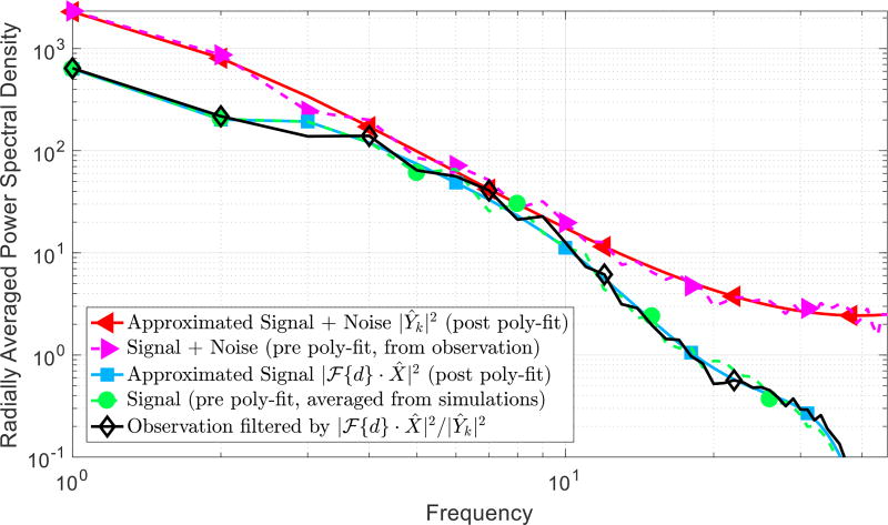
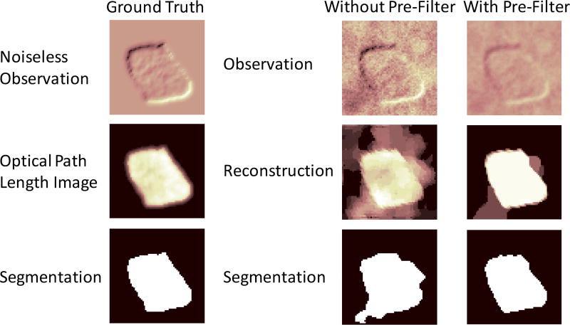
where F_k is the spatial Fourier spectrum of the pre-filter, ℱ{d} is the spatial Fourier transform of the DIC imaging function from Eq. (1), X̂_k is the OPL signal’s spatial Fourier spectrum estimate, N̂_k is the spatial Fourier spectrum estimate of ${\mathit{n}}_k^{\mathit{\text{organic}}}$ combined with ${\mathit{n}}_k^{\mathit{\text{sensor}}}$, and Ŷ_k is the signal-plus-noise’s spatial Fourier spectrum estimate. We estimate all spatial Fourier spectra using least-squares polynomial fits of the radially averaged power spectral density (RAPSD), defined as a radial averaging of the DC-centered spatial-frequency power spectrum density. Intuitively, this estimates an image’s underlying spectrum via a form of direction-unbiased smoothing. Specifically, we estimate the signal-only component X̂_k from averaged RAPSDs from OPLs of simulated cells generated from the realistic simulation framework described in Appendix A, and we estimate the combined signal-plus-noise spectra Ŷ_k from RAPSDs of observed images y_k. Fig. 3 illustrates the estimation process and effect of the pre-filter in the frequency domain. The positive contribution of the pre-filter is highlighted in Fig. 4 in the segmentation algorithm to be described next.

Fig. 3.

Radially averaged power density spectrum (RAPSD) plots in logscale from an example 64 × 64 cell patch. The Wiener filter utilizes an approximation to the signal (in blue) and the signal-with-noise (in red) power spectral density modeled as a linear polynomial least-square fitting over the radially averaged power spectral density (RAPSD). The signal approximation is computed by averaging the power spectral density of simulated cells. The signal-with-noise approximation is extracted from an observed patch. The final filtered spectrum is shown in black.

Fig. 4.

Positive contribution of pre-filtering seen as interference-suppression. The first column of images pertain to the ground truth simulation. The second and third columns pertain to PF+RWTV-DF performed without and with the pre-filter respectively. While the pre-filter blurs high frequency interference content, it also blurs the cell’s edges. We consider this an acceptable trade-off that we can thereafter comfortably recover from, using our proposed deconvolution method. The pre-filtered observation has its edge integrity retained while suppressing surrounding interference found at the bottom left corner and immediate right of the cell; this results in an overall segmentation that is closer to the ground truth.

2) RWTV-DF

Given the edge-sparse nature of the data and our particular need for accuracy in the cell membrane locations during segmentation (in contrast to the more typical MSE minimization of the deconvolved image), we use the TV norm as the core regularization approach [46] for this algorithm. Specifically, we calculate isotropic TV as:

$${\Vert {\mathit{x}}_k\Vert }_{\mathit{\text{TV}}}=\sum _{i=1}^N{\Vert {\mathit{T}}_i{\mathit{x}}_k\Vert }_2=\sum _{i=1}^N{\mathit{t}}_k[i],$$

where T_i ∈ ℝ^{2 × N} is an operator that extracts the horizontal and vertical forward-differences of the i-th pixel of x_k into an ℝ² vector, whose ℓ₂ norm we denote as an individual edge-pixel t_k[i]. This basic regularizer was improved in [31] via an iterative estimation of weights on the individual edges through an Majorize-Minimization algorithm. While effective, this regularizer does not incorporate any dynamical information for the tracking of moving edges.

To address this issue, we draw inspiration from [32], [33] and develop a hierarchical Bayesian probabilistic model where dynamics are propagated via second-order statistics from one time step to the next, the key difference being our proposed method operates solely in the edge-pixel space. To give intuition first, we note that the sparse edge locations at the previous frame is strong evidence that there will be an edge nearby in the current frame. We model edge locations with a sparsity-inducing probability distribution with a parameter controlling the spread (i.e., variance) of the distribution. When previous data gives evidence for an edge in a given location, we adjust the parameter to increase the variance of the prior in this location, thereby making it easier for the inference to identify the presence of the edge from limited observations. In contrast, when previous data indicates that an edge in a location is unlikely, this variance is decreased thereby requiring more evidence from the observations to infer the presence of an edge. For more details about this general approach to dynamic filtering (including its enhanced robustness to model uncertainty) see [33].

In detail, at the lowest level of the hierarchy, we model the pre-filtered observations conditioned on the OPL signal x_k with a white Gaussian distribution:

$$p({\mathit{F}}_k{\mathit{y}}_k|{\mathit{x}}_k)\propto e^{-\frac{1}{2{\sigma }^2}{\Vert {\mathit{F}}_k{\mathit{y}}_k-{\mathit{\text{Dx}}}_k\Vert }_2^2},$$ (7)

where F_k is the matrix operator describing 2D convolution (in the frequency domain) against the pre-filter F_k described earlier by Eq. (6). At the next level, the individual edge-pixels t_k[i] are assumed sparse and therefore best modeled with a distribution with high kurtosis but with unknown variance. Conditioning on a weighting γ_k[i] that controls the individual variances, we model t_k[i] as random variables arising from independent Laplacian distributions:

$$p({\mathit{t}}_k[i]|{\mathit{\gamma }}_k[i])={\gamma }_0\frac{{\mathbf{\gamma }}_k[i]}{2}{e}^{-{\gamma }_0{\mathbf{\gamma }}_k[i]·|{\mathit{t}}_k[i]|},$$ (8)

where γ₀ is a positive constant. At the top-most level, the weights γ_k[i] are themselves also treated as random variables with a Gamma hyperprior:

$$p({\mathit{\gamma }}_k[i]|{\mathit{\theta }}_k[i])=\frac{{\mathit{\gamma }}_k^{\alpha -1}[i]}{{\mathit{\theta }}_k^{\alpha }[i]\mathbf{\Gamma }(\alpha )}{e}^{-{\mathit{\gamma }}_k[i]/{\mathit{\theta }}_k[i]},$$ (9)

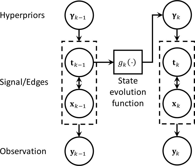
where α is a positive constant, Γ(·) is the Gamma function, and θ_k[i] is the scale variable that controls the Gamma distribution’s mean and variance over γ_k[i]. We will use this top level variable to insert a dynamics model into the inference that controls the variance of the prior being used to infer edge locations based on previous observations. Fig. 5 illustrates the multiple prior dependencies of the hierarchical Laplacian scale mixture model described in Eq. (7,8,9) using a graphical model.

Fig. 5.

Graphical model depicting the hierarchical Laplacian scale mixture model’s Bayesian prior dependencies in the RWTV-DF algorithm. Prior state estimates of the signal edges are used to set the hyper-priors for the second level variables (i.e., variances of the state estimates), thereby implementing a dynamical filter that incorporates edge information into the next time step.

To build dynamics into the model, we observe that the Gamma distribution’s scale variable θ_k[i] controls its expected value (i.e.,𝔼[γ_k[i]] = αθ_k[i]). Inspired by [33], we designed a dynamic filtering approach to the problem of interest by using a dynamics model on the edge-pixels that sets the individual variances θ_k[i]’s according to predictions from the dynamics model g_k(·):

$${\theta }_k[i]=\frac{\xi }{|g_k({\mathit{t}}_{k-1})[i]|+\eta },$$

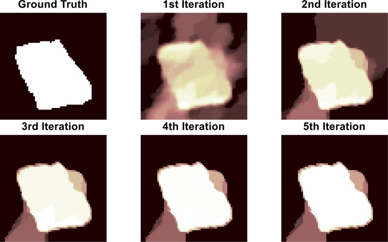
where ξ is a positive constant and η is a small constant that prevents division by zero. To illustrate the operation of this model, a strong edge-pixel in a previous frame (i.e., a large value of t_k−1[i]) sets a small value of θ_k[i] (and respectively a small expected value of γ_k[i]), in turn making the Laplacian’s variance large (i.e., Var [t_k[i]] = 2/(γ₀γ_k[i])²). A large Laplacian variance implies a higher likelihood that the edge-pixel in the current frame is active (in contrast to the reverse situation where a weak edge pixel would result in a small Laplacian variance at the next time step). Therefore, this approach propagates second-order statistics (similar to classic Kalman filtering for Gaussian models) through the hyperpriors γ_k using dynamic information via the evolution function g_k(·) at each time-step. One option for g_k(·) is a convolution against a Gaussian kernel (with its σ proportional to expected motion variation), which expresses a confidence neighborhood of edge locations based on previous edge locations [47]. As with any tracking algorithm, the tracking quality depends on the accuracy of the dynamics model and including better models (e.g., more accurate motion speeds, motion direction information based on pipette movement, etc.) would improve the performance of any approach. With a fixed dynamics function, for each frame the algorithm will take a re-weighting approach where multiple iterations are used to adaptively refine the estimates at each model stage (illustrated for a simulated patch in Fig. 6).

Fig. 6.

The ground truth image is the binary mask of a simulated image. Subsequent images reflect the iterations of reweighting process during deconvolution (iterations 1 through 5 respectively). Over the iterations, dominant edges are enhanced while weaker ones recede, resulting in piecewise smooth solutions that are amenable to segmentation.

The final optimization follows from taking the MAP estimate for Eq. (7,8,9) and applying the EM approach to iteratively update the weights. The maximization step is given as a convex formulation

$${\hat{\mathit{x}}}_k^{(t)}=\text{arg}\underset{\mathit{x}\ge \mathbf{0}}{\text{min}}-\text{log }[p(\mathit{x}|{\mathit{\gamma }}_k^{(t)})]=\text{arg}\underset{\mathit{x}\ge \mathbf{0}}{\text{min}}\frac{1}{2}{\Vert {\mathit{F}}_k{\mathit{y}}_k-\mathit{\text{Dx}}\Vert }_2^2+{\gamma }_0\sum _{i=1}^N{\mathit{\gamma }}_k^{(t)}[i]·{\Vert {\mathit{T}}_i{\mathit{x}}_k\Vert }_2.$$ (10)

The expectation step may be derived using the conjugacy of the Gamma and Laplace distributions, admitting the closed-form solution

$$=\frac{\underset{\kappa +1}{{\mathit{\gamma }}_k^{(t+1)}[i]={𝔼}_{p(\gamma |{\hat{\mathit{t}}}_k^{(t)}[i])}[\gamma ]}}{\kappa ·|{\hat{\mathit{t}}}_k^{(t)}[i]|+|g_k({\hat{\mathit{t}}}_{k-1})[i]|+\eta },$$ (11)

where the EM iteration number is denoted by superscript t, ${\hat{\mathit{t}}}_k^{(t)}[i]={\Vert {\mathit{T}}_i{\hat{\mathit{x}}}_k^{(t)}\Vert }_2$ is the estimate of the edge at iterate t, ${\hat{\mathbf{t}}}_{k-1}[i]={\Vert {\mathit{T}}_i{\hat{\mathit{x}}}_{k-1}\Vert }_2$ is the estimate of the edge at the previous time-step, γ₀ is the positive constant that controls the weight of edge-sparsity against reconstruction fidelity, and κ is the positive constant that controls the weight of the current observation against the dynamics prior. The Gaussian convolution implemented by g_k(·) effectively “smears” the previous time-step’s estimation of edges to form the current prior, accounting for uncertainty due to cell movement over time. The EM algorithm is initialized by setting all weights to 1 (i.e., ${\gamma }_k^{(0)}=1$) and solving Eq. 10, which is simply (non-weighted) TV-regularized least squares. The reweighting iterations are terminated upon reaching some convergence criteria (e.g., ‖x^(t) − x^(t−1)‖₂/‖x^(t)‖₂ < ε or after a fixed number of reweights).

C. Pipette removal via inpainting

When the pipette draws near to a cell for patching, the pipette tip in the image patch can cause significant errors in the deconvolution process. We propose a simple yet effective extension of the proposed PF+RWTV-DF algorithm that requires only a minor modification of Eq. (10). Specifically, we propose an inpainting approach [48] that masks away the pipette’s pixels and infers the missing pixels according to the same inverse process used for deconvolution. To begin, we track the pipette location in the image with a similar template matching process as described in section III-A (which could be improved with positional information from the actuator if available). Simultaneously, an associated pipette mask (obtained either via automatic segmentation or manually drawn) is aligned and overlaid on top the cell image patch using the updated pipette locations. This pipette mask overlay takes the form of a masking matrix M ∈ {0, 1}^{M × N} whose rows are a subset of the rows of an identity matrix, and whose subset is defined by pixel indices outside the pipette region. The original filtered observation F_ky ∈ ℝ^N is reduced to MF_ky ∈ ℝ^M (with M ≤ N) while the convolution operator becomes MD. The inpainting version of Eq. (10) is

$${\hat{\mathit{x}}}_k^{(t)}=\text{arg}\underset{\mathit{x}\ge \mathbf{0}}{\text{min}}\frac{1}{2}{\Vert {\mathit{\text{MF}}}_k{\mathit{y}}_k-\mathit{\text{MDx}}\Vert }_2^2+{\gamma }_0\sum _{i=1}^N{\gamma }_k^{(t)}[i]{\Vert {\mathit{T}}_i\mathit{x}\Vert }_2.$$ (12)

Intuitively, we simply remove pixels in the pipette region from the data used in the deconvolution but allow the algorithm to infer pixel values consistent with the statistical model used for regularization.

IV. Results

A. Experimental Conditions

We evaluate the performance our algorithm by using a cell simulator that generates synthetic DIC imagery of rodent neurons in brain slices. In this subsection, we present the simulation framework and demonstrate its realism by comparisons against data.

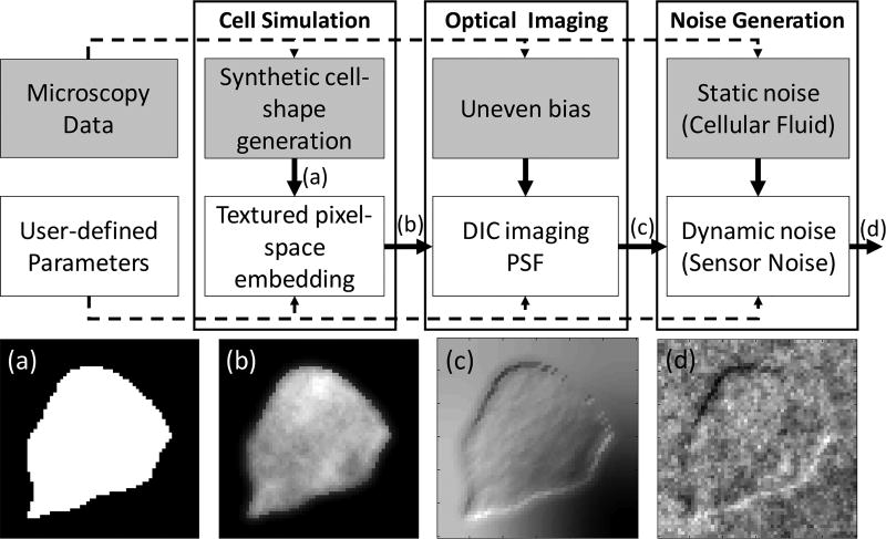
Most cell simulators can be described as having three distinct stages: cell-shape generation, optical imaging, and noise generation. The simulation framework implemented for this work uses these same three stages (shown in Fig. 7), adapting general approaches used in the literature for each stage so that the simulated data reflects the statistics of the DIC microscopy images for in vitro brain slice electrophysiology. In the first stage, a synthetic cell-shape is generated and embedded into the pixel-space as an ideal OPL image (i.e., the ground truth). In the second stage, the OPL image is transformed using a convolution against an idealized point spread function that approximately describes the DIC microscope’s optics. Lastly, interference from static components (e.g., organic material) and dynamic noise components (e.g., the image acquisition system) are generated and incorporated into the image during the third stage. In this work we have used existing general approaches to build and validate the model components in the simulator using real DIC imagery of in vitro brain slices from adult (P50–P180) mice as described in [49]. Note that this simulator is unique in that it is tailored to simulate this type of cells. Given the similarity to frameworks already existing in the literature, full implementation details for this simulator are located in Appendix A to streamline readability.

Fig. 7.

Block diagram of the cell simulator. Gray blocks: generative models that learn from available data. White blocks: generative models that rely on user-parameters. The respective images are outputs from the various stages of the simulator, including (a) Binary image of synthetic cell shape (b) Textured OPL image showing light transmission through tissue (c) Received image through DIC optics (d) Final image with noise and interference.

To evaluate the realism of synthetically generated cell-shapes, we compared several of their shape features to actual hand-drawn cell shapes from rodent brain slice imagery using four dimensionless shape features:

1. Aspect Ratio is defined as the ratio of minor axis lengths to major axis lengths. The major/minor axis is determined from the best fit ellipsoid of the binary image.

2. Form factor (sometimes known as circularity) is the degree to which the particle is similar to a circle (taking into consideration the smoothness of the perimeter [50]), defined as $\frac{4\pi A}{P^2}$, where A is area and P is the perimeter.

3. Convexity is a measurement of the particle edge roughness, defined as $\frac{P_{\text{cvx}}}{P}$, where P_cvx is the convex hull perimeter and P is the actual perimeter [51].

4. Solidity is the measurement of the overall concavity of a particle, defined as $\frac{A}{A_{\text{cvx}}}$, where A_cvx is the convex hull area and A is the image area [51].

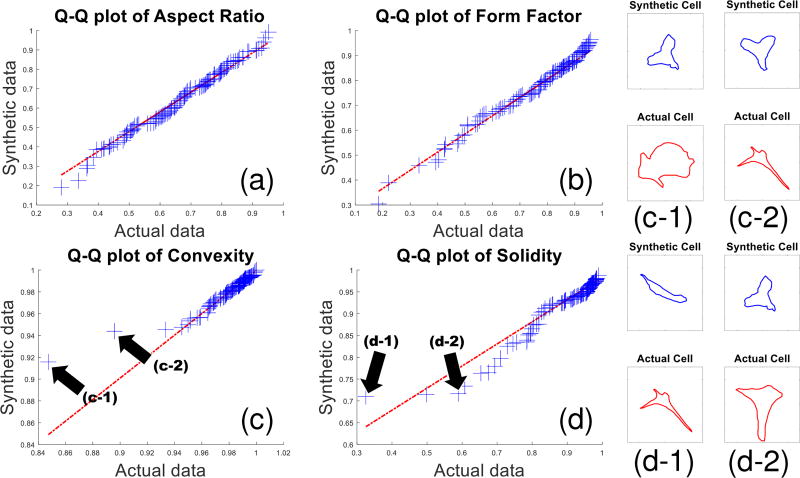
Using 50 shape-coordinates per cell we generated 115 synthetic cells. The quartile-quartile plots in Fig. 8 show that all four features are similarly distributed, demonstrating that the simulation renders realistic cell shapes for rodent in vitro brain slices.

Fig. 8.

The quantile-quantile plots visualize similarities between the characteristics of simulated and actual cell-shapes. Distributions were compared for the following shape-features: (a) aspect ratio, (b) form factor, (c) convexity, and (d) solidity as defined in the text. (c-1,c-2,d-1,d-2) Several outlier pairs from the convexity and solidity plots are identified and shown. The outlier pairs appear to be caused by actual cell shape outlier statistics that are underrepresented (due to lack of training examples) and thus not fully captured by the model.

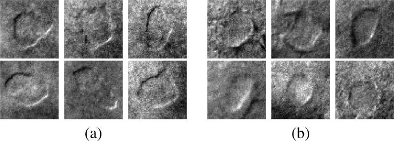
Several simulation images were generated in Fig. 9 for visual comparison against actual cell images. The following user-defined parameters (as defined in Table I found in Appendices) were used: image size was 60 × 60, cell-rotation (θ_rot) was randomized, cell-scaling defined as factor of image width was γ_scale = 0.8, DIC EPSF parameters were {θ_d = 225°, σ_d = 0.5}, dynamic noise parameters were {A_g = 0.98, σ_g = 0.018, A_p = 20.6, λ_p = 10⁻¹⁰}, and SNR χ = −1 dB. Cell shapes were randomly generated based on learned real cell-shapes, a lighting bias was taken randomly from actual image patches, and organic noise was generated using a RAPSD curve learned from real DIC microscopy images. In general, the synthetic and actual cells are qualitatively similar in cell shapes and noise textures.

Fig. 9.

General qualitative similarity between randomly drawn samples of (a) synthetically generated DIC cell images using the proposed simulator, and (b) actual DIC microscopy images of rodent neurons. Similarities in imagery characteristics include: (1) DIC optical features as shown by the 3D relief which are highlighted by the high/low intensity ‘shadows’ in the cell edges, (2) organic interference which appears as Gaussian noise with a frequency profile (further elaboration on quantitative similarities are found in Appendix A-C2), (3) cell shapes as demonstrated by the cell shapes’ organic and natural contours, and (4) uneven lighting bias as shown by the smooth but uneven background gradient.

B. Segmentation of synthetic data

We test the PF+RWTV-DF algorithm on synthetic cell data and compare its performance against the state-of-the-art deconvolution algorithms such as least-squares regularized by ℓ₁ and TV (L1+TV) [20], least-square regularized by ℓ₁ and Laplacian Tikhonov (L1+Tik) [20], and least-square by regularized re-weighted ℓ₁, weighted Laplacian Tikhonov, and weighted dynamic filtering (RWL1+WTik+WDF) [30]. The deconvolution from each algorithm is then segmented using a global threshold (using Otsu’s method [45]) to produce a binary image mask for algorithmic evaluation.

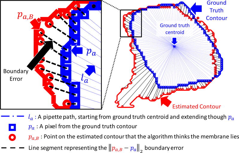
For evaluation, we employ three boundary metrics that capture errors relevant to the process of patch clamping. The metrics Average Boundary Error (ABE), Maximum Boundary Error (MBE), and Variance of Boundary Errors (VBE) measure the (average, maximum, and variance of) distance errors between the approximated cell boundary and the actual cell boundary around the entire membrane of the cell at each video frame. Specifically, these metrics capture the statistics of the distance errors between the actual and estimated cell boundaries as the pipette tip approaches the cell membrane in a straight path (directed towards the true centroid).

To compute these metrics, we first discretized potential pipette paths towards the true centroid using a set of lines {l_a}, defined as lines that start at the true centroid and that infinitely extend through each point p_a in the set of ground truth contour pixels {A}. Next, traveling along each l_a toward the centroid we found the intersecting point in the set of estimated contour pixels {B}, defined as p_a,B = arg min_pb∈B ‖p_b − p_l‖₂ s.t. p_l ∈ l_a, where p_l are points on the line l_a. In other words, we found the points that the algorithm would identify as the membrane location during every hypothetical approach direction of the pipette. The ‖p_b − p_l‖₂ in the objective considers only orthogonal projections of p_b unto the line l_a (since it is a minimization), and it searches over all of B to find the p_b whose orthogonal projection distance is minimal. Note that that due to the contour discretization, p_a,B does not lie exactly along l_a but rather close to it on some p_b ∈ B. With each discretized boundary error expressed as ε(a,B) = ‖p_a,B − p_a‖₂, the metrics are then defined as:

$$\text{ABE}(A,B)=\frac{1}{{\Vert A\Vert }_0}\sum _{a\in A}\epsilon (a,B)$$

$$\text{MBE}(A,B)=\underset{a\in A}{\text{max }}\epsilon (a,B)$$

$$\text{VBE}(A,B)=\frac{1}{{\Vert A\Vert }_0-1}\sum _{a\in A}{(\epsilon (a,B)-\text{ABE}(A,B))}^2.$$

Fig. 10 illustrates the terms involved in these error metric computations.

Fig. 10.

Illustration of boundary error metrics. Each blue line l_a represents an approach direction of a pipette towards the ground truth centroid. p_a,B represents the point where the algorithm thinks the membrane is. Individual boundary errors are computed as the distance ‖p_a,B−p_a‖₂ and represented as black dotted lines. The average of all errors constitutes the Average Boundary Error (ABE), the maximum constitutes the Maximum Boundary Error (MBE), and the variance of errors constitutes the Variance of Boundary Errors (VBE).

We generated 100 videos of synthetic cell patches (each video contains 64×64 pixels × 100 frames) using the proposed cell simulator with DIC EPSF parameters σ_d = 0.5 and θ_d = 225° (assumed to be known either by visual inspection (to accuracy of ±15°) or more accurately by using a calibration bead [22]). By physically relating real cells to simulated cells, we determined the relationship between physical length and pixels to be approximately 3.75 pixels per 1.0µm.

For the algorithms L1+TV (Eq. (2)), L1+Tik (Eq. (3)), and RWL1+WTik+WDF (Eq. (4)), the parameters for sparsity (β) and smoothness (γ) were tuned via exhaustive parameter sweep on the first frame of the video (to find the closest reconstruction/deconvolution by the ℓ₂ least squares sense). Specifically, the sweep was conducted over 10 logarithmically spaced values in the given ranges: L1+TV searched over [10⁻³, 10⁻⁹] for β and [10⁻¹, 10⁻⁵] for γ, L1+Tik searched over [10⁻³, 10⁻⁹] for β and [10⁻¹, 10⁻⁷] for γ, and RWL1+WTik+WDF searched over [10⁻³, 10⁻⁹] for β and [10⁻¹, 10⁻⁵] for γ. L1+Tik (the non-reweighted version) was used in all experiments because it was experimentally found to be better performing compared to the reweighted version (i.e., set Λ = I for Eq. (3)); reweighting over-induces sparsity of pixels, which is not advantageous to segmentation in our particular application. For RWL1+WTik+WDF, the dynamics parameter was set to be κ = 1.0 × 10⁻³, with a maximum of 80 reweighting steps (where convergence is fulfilled before each reweighting). For PF+RWTV-DF (Eq. (10, 11)), we fixed γ₀ = 3.0×10⁻⁴, κ = 5, with 4 reweighting steps (where convergence is fulfilled before each reweighting). The programs specified by L1+TV, RWL1+WTik+WDF, and PF+RWTV-DF were solved using CVX [52], [53], while L1+Tik was solved using TFOCS [54].

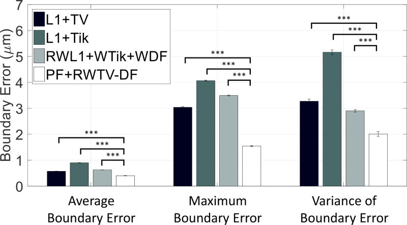
Fig. 11 reflects statistics of the respective algorithms from each of the 100 frames from the 100 video trials. The height of each bar refers to the average of ABE/MBE/VBE while the error bars refer to ±1 standard error of the ABE/MBE/VBE over the 100 video trials. PF+RWTV-DF was the best performing algorithm in the three metrics, and there is a significant difference (p ≤ 0.001) between PF+RWTV-DF and the other algorithms for all metrics. Notably, PF+RWTV-DF results in boundary tracking errors on the order of 1–2 µm, which is comparable to the error in mechanical pipette actuators.

Fig. 11.

Average boundary errors (ABE), maximum boundary errors (MBE), and variance of boundary errors (VBE) for each of the algorithms across 100 video trials of simulated data. ABE/MBE/VBE was aggregated from 100 frames of 100 trials (i.e., 10,000 data points). The PF+RWTV-DF algorithm was found to have a state-of-the-art performance, showing statistically significant improvements in ABE/MBE/VBE compared to other algorithms (p ≤ 0.001, denoted by the 3 stars based on paired t-tests).

The proposed edge reweighing strategy is adaptive by design, making it very attractive in practice because it requires minimal parameter fine-tuning. The algorithm’s performance was responsive to the smoothness parameter (effective range being γ ∈ [2.0 × 10⁻⁴, 4.0 × 10⁻⁴]) and the dynamics parameter (effective range being κ ∈ [10⁰, 10²]), yet not over-sensitive: our algorithm’s superior results were from fixed parameters (γ, κ) across all trials, while other algorithms required exhaustive two-parameter sweeps (β, γ) for each synthetic video trial.

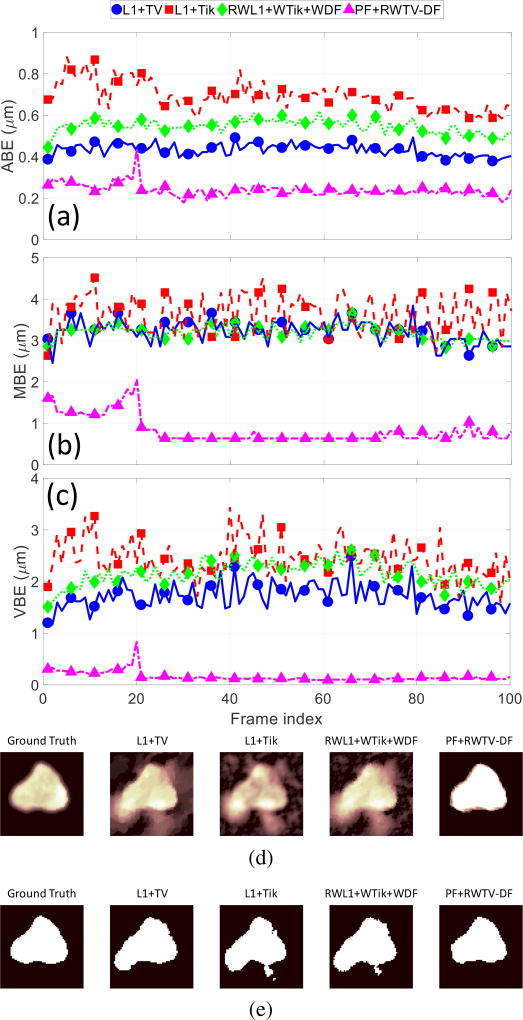
In Fig. 12 we take a closer look at one representative trial (Trial #4) in the time-series to observe the qualitative differences between the algorithms. We observe that the PF+RWTV-DF reconstruction has a fairly flat magnitude (for pixel values within the cell) compared to the other reconstructions. The proposed algorithm’s inherent segmentation capability under such high-interference synthetic data is apparent from these results. Although PF+RWTV-DF reconstruction loses cell details (i.e., in an ℓ₂ reconstruction sense), the reduction in surrounding interference serves to improve the boundary identification at the segmentation stage. On the other hand, the other algorithms produce reconstructions that contain significant surrounding interference, resulting in distorted edges in their subsequent segmentations (that may require further image processing to remove). Video showing the deconvolution and tracking time series is included in a multimedia supplement to this paper.

Fig. 12.

ABE, MBE, and VBE evolving with time are shown from (a) to (c) (respectively) for a single representative video (Trial #4) of a simulated DIC microscopy cell with 100 video frames after deconvolution and segmentation using four different algorithms. The images in (d) are snapshots of the deconvolution output at frame 100, and the images in (e) are their respective segmentations.

C. Segmentation of real data

In addition to the synthetic data where we have known ground truth, we also tested the algorithms on in vitro DIC microscopy imagery of rodent brain slices from the setup described in [49]. For each algorithm, a parameter search was performed using a brute-force search to find the parameters that best segmented the cell by means of visual judgement. The DIC EPSF was estimated visually to be σ_d = 0.5, θ_d = 225°.

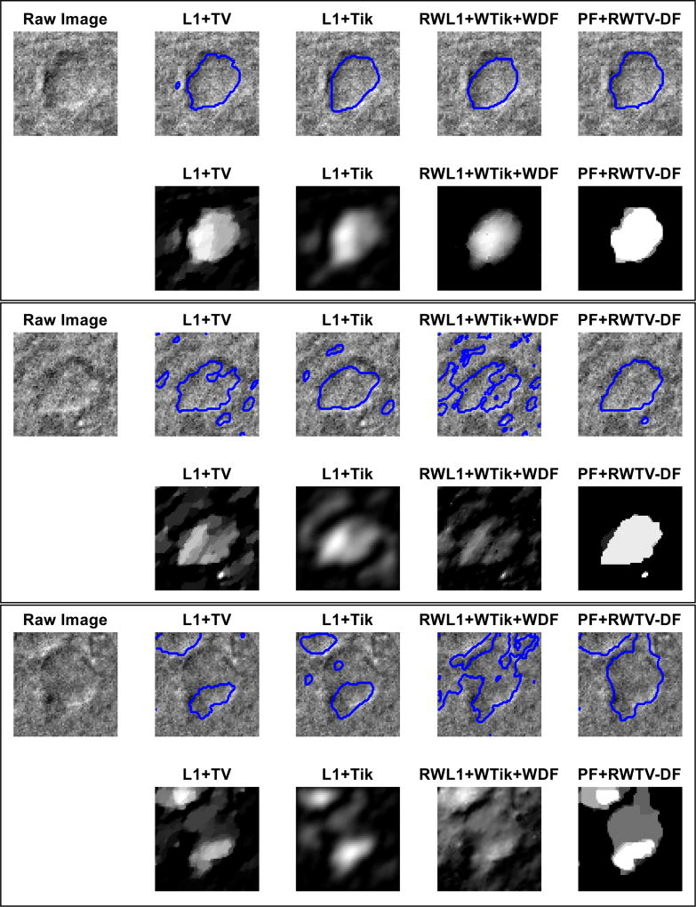
In Fig. 13, we selected 3 particularly challenging cell samples with respect to the amount of observable interference around and within the cell. A fixed global threshold was applied to each patch for segmentation using Otsu’s method [45]. The first example (from the top) demonstrates that reconstructions of other algorithms (compared to the proposed algorithm) are characteristically not piecewise smooth. Therefore, even in a case of moderate difficulty such as this one, these algorithms produce images with rounded edges which are not ideal for segmentation. The second example illustrates difficulty in segmenting cells with significant interference along the cell’s edges, around the outside of the cell, and within the body of the cell. In this case, only the proposed algorithm is able to produce a clean segmentation, especially along the cell’s edges. Moreover, other algorithms reproduce the heavy interference scattered around the outside of the cell and this requires subsequent image processing to remove. The third example is a very difficult case where interference occurs not only as distorted boundaries, but also as a close neighboring cell. All other algorithms visibly perform poorly while the proposed algorithm remains fairly consistent in its performance.

Fig. 13.

Three example image patches of real cell data were deconvolved using four algorithms and the resulting segmentations (top row) and deconvolutions (row below) are displayed. Segmentations were obtained from deconvolution by global thresholding using Otsu’s method [45]. The proposed PF+RWTV-DF algorithm performs consistently well even in severe interference (defined by the degree of distortion around the edges and surface undulations within the cell).

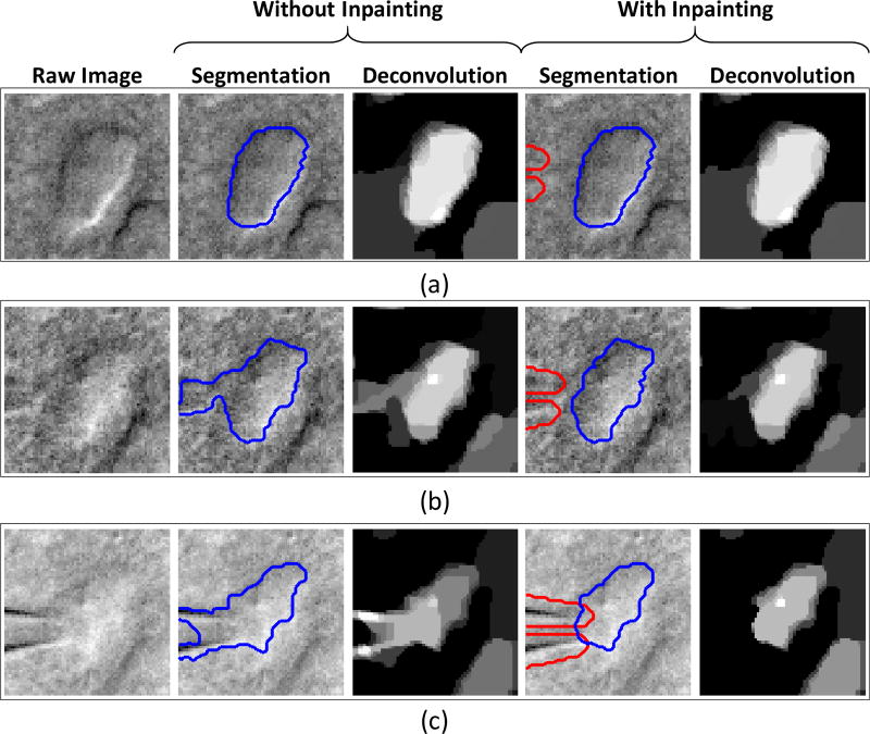
In Fig. 14, snapshots from a video of a cell undergoing patch clamping was compared with and without the proposed pipette removal method (from section III-C). The pipette (and its respective mask) was tracked using a template matching algorithm via a user-selected template of the pipette; more details are described in [44]. In Fig. 14(a), the pipette does not cause interference when it is relatively far away from the cell. As the pipette approaches the cell in Fig. 14(b), interference begins to enter the deconvolution when inpainting is not applied. Without inpainting, an obfuscation between the pipette and the cell is observed in the deconvolution even when the pipette is not overlapping with the cell. In Fig. 14(c), the pipette is now seen to be overlapping the cell image. Without inpainting, this causes such severe interference that attempting a pipette removal at the segmentation stage is clearly non-trivial. With inpainting, the deconvolution is shown to effectively suppress the interfering pipette in all three snapshots.

Fig. 14.

Snapshots from real video data of a cell undergoing patch clamping demonstrate the efficacy of the proposed pipette removal method (via inpainting). The pipette mask is outlined in red while the cell segmentation is outlined in blue. Each snapshot illustrated varying degrees of overlap between the pipette and the cell: (a) the pipette is far from the cell, (b) the pipette is in close proximity to the cell, and (c) the pipette is “touching” the cell. The efficacy of the proposed inpainting method for pipette removal (versus no inpainting) is qualitatively demonstrated by its ability to cleanly segment the cell despite the pipette’s presence.

V. Conclusion

We present the first deconvolution algorithm to locate cell boundaries with high precision in DIC microscopy images of brain slices. In summary, the main technical contributions of this algorithm are: (1) a pre-filtering step that is a computationally cheap and effective way at removing heavy organic interference with spectral characteristics, (2) a dynamical ℓ₁ reweighing approach for the propagation of second-order edge statistics in online DIC cell segmentation, and (3) an inpainting approach for pipette removal that is possible with little modification due to the inherently flexible framework of the algorithm. To quantitatively validate the performance of segmentation algorithms, this paper also describes the novel adaptation of cell simulation techniques to the specific data statistics of DIC microscopy imagery of brain slices in a publicly available MATLAB toolbox.

The proposed algorithm achieves state-of-the-art performance in tracking the boundary locations of cells, with the average and maximum boundary errors achieving the desired tolerances (i.e., 1–2 µm) driven by the accuracy of actuators used for automatic pipette movement. These results lead us to conclude that accurate visual guidance will be possible for automated patch clamp systems, resulting in a significant step toward high-throughput brain slice electrophysiology. The main shortfall of the proposed algorithm arises from the implicit assumption that dynamics are spatially limited. In order for dynamics to positively contribute to the deconvolution process, edges in the current frame should fall within the vicinity of the previous frame’s edges; specifically, it should be bounded by the support of the prediction kernel as described by Eq. (11). Future work aims at developing a real-time numerical implementation of this algorithm using parallelization methods such as alternating direction methods of multipliers (ADMM) similar to work found in [55], [56], exploring the inclusion of shape-regularizers [57]–[59] into the optimization, investigating alternative methods that incorporate dynamics in a fashion that is not spatially-limiting, and characterizing dynamical functions that take into account physical models of motion in the system (e.g., motion induced by the pipette, fluid dynamics, cell deformation physics).

Biographies

Christopher J. Rozell Christopher J. Rozell (S’00–M’09–SM’12) received the B.S.E. in Computer Engineering and the B.F.A. in Performing Arts Technology (Music Technology) in 2000 from the University of Michigan, Ann Arbor. He attended graduate school at Rice University where he was a Texas Instruments Distinguished Graduate Fellow, receiving the M.S. and Ph.D. in Electrical Engineering in 2002 and 2007, respectively.

Following graduate school Dr. Rozell was a post-doctoral research fellow in the Redwood Center for Theoretical Neuroscience at the University of California, Berkeley. He joined the Georgia Tech faculty in July 2008, where he is currently an Associate Professor in the School of Electrical and Computer Engineering and the Associate Director of the Neural Engineering Center. In 2014, Dr. Rozell received the Scholar Award in Studying Complex Systems from the James S. McDonnell Foundation 21st Century Science Initiative, as well as a National Science Foundation CAREER Award.

John Lee received the B.Eng. degree from the Department of Electrical and Computer Engineering, National University of Singapore, in 2010, and in 2014 started the Ph.D. degree in Electrical Engineering specializing in signal processing at the Georgia Institute of Technology (Atlanta, GA). His current research interests include dynamic tracking, sparse representations, optimization, and optimal transport.

Ilya Kolb received his B.S. and M.S. degrees from the Department of Biomedical Engineering, Case Western Reserve University (Cleveland, OH) in 2012 and 2013 respectively. He received his Ph.D. degree at Georgia Institute of Technology (Atlanta, GA) in 2017. Ilya’s research interests include neural interfacing and instrumentation techniques in neuroscience. He is currently a Research Specialist at the Janelia Research Campus in Ashburn, VA.

Craig R. Forest Craig Forest is an Associate Professor and Woodruff Faculty Fellow in the George W. Woodruff School of Mechanical Engineering at Georgia Tech where he also holds program faculty positions in Bioengineering and Biomedical Engineering. He conducts research on miniaturized, high-throughput robotic instrumentation to advance neuroscience and genetic science. Prior to Georgia Tech, he was a research fellow in Genetics at Harvard Medical School. He obtained a Ph.D. in Mechanical Engineering from MIT in June 2007, M.S. in Mechanical Engineering from MIT in 2003, and B.S. in Mechanical Engineering from Georgia Tech in 2001. He is cofounder/organizer of one of the largest undergraduate invention competitions in the USThe InVenture Prize, and founder/organizer of one of the largest student-run makerspaces in the USThe Invention Studio. He was a recently a Fellow in residence at the Allen Institute for Brain Science in Seattle WA; He was named Engineer of the Year in Education for the state of Georgia (2013) and was a finalist on the ABC reality TV show “American Inventor.”

Appendix A

Simulation Framework

A. Simulation Stage 1: Cell Shape Generation

The cell-shape is unique to different applications and plays a significant role in algorithm development, necessitating customization in cell simulations [35], [60]. Extensive work on generic shape representation in [60] demonstrated that applying principal components analysis (PCA) on cell-shape outlines is an excellent strategy for reconstructing cell shapes. In this work, we applied a similar approach as [35] to generate synthetic cell-shapes using PCA and multivariate kernel density estimation sampling on subsampled cell contours. For shape examples, we used hand drawn masks of neurons from DIC microscopy images of rodent brain slices.

Example cell-shapes are collected such that K coordinates are obtained in clockwise continuous fashion (around the contour), beginning at the north-most point. These points are centered such that the centroid is at the origin. The (x, y) coordinates are concatenated into an ℝ^d vector

$${\mathit{x}}_i={(x_1,\dots ,x_K,y_1,\dots ,y_K)}^{\top },$$

where d = 2K. This vector is then normalized via x̂_i = x_i/‖x_i‖₂. All N normalized examples are gathered into the following matrix

$$\mathit{X}=({\hat{\mathit{x}}}_1,\dots ,{\hat{\mathit{x}}}_N).$$

Eigen-decomposition is performed on the data covariance matrix formed as S = XX^T = VΛV^T. Cell-shapes may thus be expressed with the coefficient vector b_i and the relationship given by

$${\mathit{x}}_i={\mathit{\text{Vb}}}_i\iff {\mathit{b}}_i={\mathit{V}}^{\top }{\mathit{x}}_i.$$ (13)

Since PCA guarantees that cov(b_i, b_j) = 0, ∀i ≠ j, kernel density estimation is performed individually on each of the coefficients to estimate its underlying distributions. This allows us to randomly sample from these distributions to produce a synthetically generated coefficient vector, b̃. The cell-shape may then be trivially converted into coordinates using the relationship given in Eq. (13). A rotation (θ_rot) and scaling (γ_scale) are added to the cell-shapes where necessary.

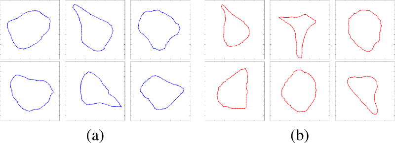
Fig. 15 shows a sampling of synthetic and actual cell-shapes extracted from the data.

Fig. 15.

Visual similarities were observed between the (a) synthetically generated cell-shapes, and the (b) cell-shapes extracted from DIC imagery of rodent brain slices.

1) Textured OPL pixel-space embedding

The previously generated cell-shape is embedded into the pixel space f_x,y by a texture generation method similar to methods found in other fluorescence microscopy simulators [61], [62]. In this stage, the cell-shape is embedded into the pixel space with the generation of a textured OPL image. Perlin noise [63] is a well-established method for generating synthetic cell textures in fluorescent microscopy [61], [62], and we apply a similar concept because it generates realistic looking cell textures.

First, a binary mask, m(x, y), is generated using the cell-shape’s coordinates as polygon vertices and cast into an M × M image. Next, a textured image, t(x, y) is generated by frequency synthesis; a 2-D filter with a 1/f^p frequency spectra is applied to white Gaussian noise, where p is a persistence term which controls the texture’s heterogeneity. t(x, y) is rescaled such that t̂(x, y) ∈ [0, 1]. Finally, the OPL image is constructed by

$$f(x,y)=(m(x,y)\ast h(x,y))·(m(x,y)·\hat{t}(x,y)),$$

where * signifies 2D convolution, and h(x, y) is a 2-D filter (e.g., a circular pillbox averaging filter) that rounds the edges of the OPL image. An example surface texture is simulated and shown in Fig. 7(b).

B. Simulation Stage 2: Optical Imaging

Microscopy optics is modeled here using two linear components: an effective point spread function (EPSF) and a lighting bias. DIC microscopy exploits the phase differential of the specimen to derive the edge representations of microscopy objects. The EPSF is approximated as a convolution of the OPL image f(x, y) against the steerable first-derivative of Gaussian kernel, in Eq. (1).

Nonuniform lighting of a microscope often causes a pronounced lighting bias in the image. As presented in [20], [64], a linear approximation of quadratic coefficients sufficiently expresses such a bias:

$$b(x,y)=p_0+p_{1}x+p_{2}y+p_3{x}^2+p_4\mathit{\text{xy}}+p_5{y}^2.$$ (14)

An example noiseless simulated image with the optical imaging model (including EPSF convolution and lighting bias) is shown in Fig. 7(c). Polynomials p₀, …, p₅ are estimated from a randomly extracted patch from an actual DIC image using a least-squares framework detailed in [20].

C. Simulation Stage 3: Noise Generation

1) Synthetic noise generation framework

Noise in a video frame may be linearly decomposed into organic and sensor components: $n_k(x,y)=n^{\mathit{\text{organic}}}(x,y)+n_k^{\mathit{\text{sensor}}}(x,y)$, with κ denoting the frame index in time. We define n^organic(x, y) as the components comprising of organic contributions in the specimen (e.g., cellular matter, fluids) that remain static frame-to-frame, while $n_k^{\mathit{\text{sensor}}}(x,y)$ refers to noise from the CCD that is iid across every pixel and frame. For the purpose of statistical estimation, we selected sequences of image frames {y_k(x, y)}_k=1,…,K that represented noise only (i.e., no target cell) with no tissue motion from pipette insertion. We estimate the organic noise component by averaging a series of image frames (to reduce sensor noise):

$$n^{\mathit{\text{organic}}}(x,y)\approx \overline{y}(x,y)=\frac{1}{K}\sum _{k=1}^K{y}_k(x,y).$$

Similarly, a sensor noise sample may be estimated by subtracting the the frame-average from the individual frame:

$$n_k^{\mathit{\text{sensor}}}(x,y)\approx y_k(x,y)-\overline{y}(x,y).$$

2) Organic Noise

We employ a spectral analysis framework to model and generate realistic looking interference caused by organic tissue. We define the radially averaged power spectral density (RAPSD), P(f), as an averaging of the power spectral density (PSD) magnitudes along a concentric ring (whose radius is proportional to frequency, denoted by f) on a DC-centered spatial PSD Fourier plot. The RAPSD of random noise images reveal spectral characteristics shown in Fig. 16(d). Phase information is simulated by randomly sampling from a uniform distribution Φ(m, n) ~ Uniform([0, 2π]), with m, n representing the spatial coordinates in the DC-centered Fourier domain, while the magnitude information is composed as a mean spectra P̄(f) from RAPSD of example image patches {P_k}_k=1,…,K as

$$\overline{P}(f)=\frac{\sqrt{2}}{K}\sum _{k=1}^K{P}_k(f).$$

The organic noise spectrum is thus described by its magnitude and phase components as

$$\stackrel{\sim }{S}(m,n)=|\overline{P}(\sqrt{m^2+n^2})|\text{exp}(j·\mathrm{\Phi }(m,n)).$$

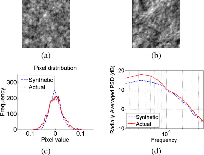
An inverse spatial Fourier transform on the organic noise spectrum yields a synthetic organic noise image: ñ^organic(x, y) = ℱ⁻¹{S̃(m, n)}. An example organic noise image patch ñ^organic(x, y) (shown in Fig. 16(a)) exhibits visual similarities with a patch of organic noise from an actual DIC image (shown in Fig. 16(b)). Additionally, similarities were observed in pixel distributions between synthetic organic noise and actual organic noise, qualitatively as shown in Fig 16(c), as well as quantitatively via a Kolmogorov-Smirnov two-sample goodness-of-fit test at the 5% significance level (after normalization by their respective sample standard-deviations).

Fig. 16.

(a) Synthetically generated organic noise (synthetic) (b) An image patch of organic noise from a real DIC image (i.e. an image patch with no cell, only noise) (c) Comparisons of pixel intensity distributions (d) Comparisons of radially averaged power spectral density.

3) Sensor noise

The CCD sensor contributes a mixture of Poisson noise and zero-mean white-Gaussian noise [62], [64]. For modeling simplicity we assume that the sensor’s individual pixels are uncorrelated in time and space, and generated using

$$n_k^{\mathit{\text{sensor}}}(x,y)=A_g·n_g+A_p·n_p,$$ (15)

where n_g ~ Normal(0, ${\sigma }_g^2$) and n_p ~ Poisson(λ_p) are randomly generated intensity values, {A_g,A_p} are amplitude parameters, and {σ_g, λ_p} are the Gaussian’s standard deviation and the Poisson’s mean parameters respectively.

D. Image and Video Synthesis

1) Image synthesis

Each simulation frame is generated as a linear combination of the various synthesized components

$$y(x,y)=\left[{10}^{\chi /10}\frac{{\Vert n(x,y)\Vert }_F}{{\Vert g(x,y)\Vert }_F}\right]·g(x,y)+n(x,y)+b(x,y),$$ (16)

where χ is a user-defined signal-to-noise ratio (in dB), and where ‖·‖_F is the Frobenius norm. Table I summarizes the user-defined parameters of this simulator.

2) Video synthesis

During the patch clamp process, pipette motion causes the cells to undergo overall translation (e.g., moving from left to right with respect to the frame), and some sequence of dilation and contraction. Videos of K image frames are generated to simulate motion of the cell (rather than the pipette itself) by evolving a single textured OPL pixel-space embedding image over time using a series of geometric transformations. Specifically, we simulate a dialation/contraction using MATLAB’s barrel transformation function [65] and apply geometric translation along a random linear path through the center of the image with a parabolic velocity profile (e.g., an acceleration followed by a deceleration). These transformations produced a set of frames {f_k(x, y)}_k=1,2,… which are convolved in 2D using Eq. (1) and synthesized using Eq. (16) to generate a set of time-varying observations {y_k(x, y)}_k=1,2,… comparable to a video sequence of DIC imagery from a patch clamp experiment. Example snapshots from a synthetic video is shown in Fig. 17.

TABLE I.

User-defined simulator parameters.

Parameter	Description
M	Image size (i.e., M × M pixel-image)
θrot	Rotation angle of cell-shape
γscale	Scaling factor of cell-shape within image
p	Persistence of OPL surface texture
{σd, θd}	DIC imaging function parameters (Eq. (1))
{Ag, σg}	Dynamic noise Gaussian parameters (Eq. (15))
{Ap, λp}	Dynamic noise Poisson parameters (Eq. (15))
χ	SNR (in dB) of final image (Eq. 16)

Fig. 17.

Four snapshots in time (indexed by k) from a synthesized video (of 100 frames), generated from a single cell image. The cell’s motion induced by external forces (i.e., pipette motion, though not explicitly present) is simulated by a slight contraction followed by expansion over time, while performing a linear translation, from left to right of the frame. Synthetic interference (simulating organic material) shows up as a high-intensity blob around the bottom left corner of the cell, interfering with the cell’s edges.

References

- 1.Vickers AE, Fisher RL. Organ slices for the evaluation of human drug toxicity. Chemico-Biological Interactions. 2004;150(1):87–96. doi: 10.1016/j.cbi.2004.09.005. [DOI] [PubMed] [Google Scholar]
- 2.Kamioka H, Honjo T, Takano-Yamamoto T. A three-dimensional distribution of osteocyte processes revealed by the combination of confocal laser scanning microscopy and differential interference contrast microscopy. Bone. 2001;28(2):145–149. doi: 10.1016/s8756-3282(00)00421-x. [DOI] [PubMed] [Google Scholar]
- 3.Mulligan SJ, MacVicar BA. Calcium transients in astrocyte endfeet cause cerebrovascular constrictions. Nature. 2004;431(7005):195–199. doi: 10.1038/nature02827. [DOI] [PubMed] [Google Scholar]
- 4.Bussek A, Wettwer E, Christ T, Lohmann H, Camelliti P, Ravens U. Tissue slices from adult mammalian hearts as a model for pharmacological drug testing. Cellular Physiology and Biochemistry. 2009;24(5–6):527–536. doi: 10.1159/000257528. [DOI] [PubMed] [Google Scholar]
- 5.Simon I, Pound CR, Partin AW, Clemens JQ, Christens-Barry WA. Automated image analysis system for detecting boundaries of live prostate cancer cells. Cytometry. 1998;31(4):287–294. doi: 10.1002/(sici)1097-0320(19980401)31:4<287::aid-cyto8>3.0.co;2-g. [DOI] [PubMed] [Google Scholar]
- 6.Wu K, Gauthier D, Levine MD. Live cell image segmentation. IEEE Trans. Biomed. Eng. 1995;42(1):1–12. doi: 10.1109/10.362924. [DOI] [PubMed] [Google Scholar]
- 7.Dufour A, Shinin V, Tajbakhsh S, Guillén-Aghion N, Olivo-Marin J-C, Zimmer C. Segmenting and tracking fluorescent cells in dynamic 3-D microscopy with coupled active surfaces. IEEE Trans. Image Process. 2005;14(9):1396–1410. doi: 10.1109/tip.2005.852790. [DOI] [PubMed] [Google Scholar]
- 8.Yang F, Mackey MA, Ianzini F, Gallardo G, Sonka M. International Conference on Medical Image Computing and Computer-Assisted Intervention. Springer; 2005. Cell segmentation, tracking, and mitosis detection using temporal context; pp. 302–309. [DOI] [PubMed] [Google Scholar]
- 9.Padfield D, Rittscher J, Thomas N, Roysam B. Spatio-temporal cell cycle phase analysis using level sets and fast marching methods. Medical Image Analysis. 2009;13(1):143–155. doi: 10.1016/j.media.2008.06.018. [DOI] [PubMed] [Google Scholar]
- 10.Dzyubachyk O, Niessen W, Meijering E. 4th IEEE International Symposium on Biomedical Imaging: From Nano to Macro, 2007. ISBI 2007. IEEE; 2007. A variational model for level-set based cell tracking in time-lapse fluorescence microscopy images; pp. 97–100. [Google Scholar]
- 11.Zimmer C, Labruyere E, Meas-Yedid V, Guillen N, Olivo-Marin J-C. Segmentation and tracking of migrating cells in videomicroscopy with parametric active contours: A tool for cell-based drug testing. IEEE Trans. Med. Imag. 2002;21(10):1212–1221. doi: 10.1109/TMI.2002.806292. [DOI] [PubMed] [Google Scholar]
- 12.Maška M, Daněk O, Garasa S, Rouzaut A, Muñoz-Barrutia A, Ortiz-de Solorzano C. Segmentation and shape tracking of whole fluorescent cells based on the Chan–Vese model. IEEE Trans. Med. Imag. 2013;32(6):995–1006. doi: 10.1109/TMI.2013.2243463. [DOI] [PubMed] [Google Scholar]
- 13.Maška M, Ulman V, Svoboda D, Matula P, Matula P, Ederra C, Urbiola A, España T, Venkatesan S, Balak DM, et al. A benchmark for comparison of cell tracking algorithms. Bioinformatics. 2014;30(11):1609–1617. doi: 10.1093/bioinformatics/btu080. [DOI] [PMC free article] [PubMed] [Google Scholar]
- 14.Ulman V, Maška M, Magnusson KE, Ronneberger O, Haubold C, Harder N, Matula P, Matula P, Svoboda D, Radojevic M, et al. An objective comparison of cell-tracking algorithms. Nature Methods. 2017 doi: 10.1038/nmeth.4473. [DOI] [PMC free article] [PubMed] [Google Scholar]
- 15.Padfield D, Rittscher J, Roysam B. Coupled minimum-cost flow cell tracking for high-throughput quantitative analysis. Medical Image Analysis. 2011;15(4):650–668. doi: 10.1016/j.media.2010.07.006. [DOI] [PubMed] [Google Scholar]
- 16.Hamill OP, Marty A, Neher E, Sakmann B, Sigworth F. Improved patch-clamp techniques for high-resolution current recording from cells and cell-free membrane patches. Pflügers Archiv European journal of physiology. 1981;391(2):85–100. doi: 10.1007/BF00656997. [DOI] [PubMed] [Google Scholar]
- 17.Stuart G, Dodt H, Sakmann B. Patch-clamp recordings from the soma and dendrites of neurons in brain slices using infrared video microscopy. Pflügers Archiv European Journal of Physiology. 1993;423(5):511–518. doi: 10.1007/BF00374949. [DOI] [PubMed] [Google Scholar]
- 18.Kodandaramaiah SB, Franzesi GT, Chow BY, Boyden ES, Forest CR. Automated whole-cell patch-clamp electrophysiology of neurons in vivo. Nature Methods. 2012;9(6):585–587. doi: 10.1038/nmeth.1993. [DOI] [PMC free article] [PubMed] [Google Scholar]
- 19.Kolb I, Stoy W, Rousseau E, Moody O, Jenkins A, Forest C. Cleaning patch-clamp pipettes for immediate reuse. Scientific Reports. 2016;6 doi: 10.1038/srep35001. [DOI] [PMC free article] [PubMed] [Google Scholar]
- 20.Li K, Kanade T. Information Processing in Medical Imaging. Springer; 2009. Nonnegative mixed-norm preconditioning for microscopy image segmentation; pp. 362–373. [DOI] [PubMed] [Google Scholar]
- 21.U. S. G. S. A. Federal Standard. Telecommunications: Glossary of telecommunication terms. 1996 Aug 7; [Online]. Available: http://www.its.bldrdoc.gov/fs-1037/fs-1037c.htm.
- 22.Van Munster E, Van Vliet L, Aten J. Reconstruction of optical pathlength distributions from images obtained by a wide-field differential interference contrast microscope. Journal of Microscopy. 1997;188(2):149–157. doi: 10.1046/j.1365-2818.1997.2570815.x. [DOI] [PubMed] [Google Scholar]
- 23.Kachouie NN, Fieguth P, Jervis E. 2008 30th Annual International Conference of the IEEE Engineering in Medicine and Biology Society. IEEE; 2008. Watershed deconvolution for cell segmentation; pp. 375–378. [DOI] [PubMed] [Google Scholar]
- 24.Ronneberger O, Fischer P, Brox T. International Conference on Medical Image Computing and Computer-Assisted Intervention. Springer; 2015. U-net: Convolutional networks for biomedical image segmentation; pp. 234–241. [Google Scholar]
- 25.Yin Z, Bise R, Chen M, Kanade T. 2010 IEEE International Symposium on Biomedical Imaging: From Nano to Macro. IEEE; 2010. Cell segmentation in microscopy imagery using a bag of local Bayesian classifiers; pp. 125–128. [Google Scholar]
- 26.Kuijper A, Heise B. 19th International Conference on Pattern Recognition, 2008. ICPR 2008. IEEE; 2008. An automatic cell segmentation method for differential interference contrast microscopy; pp. 1–4. [Google Scholar]
- 27.Obara B, Roberts MA, Armitage JP, Grau V. Bacterial cell identification in differential interference contrast microscopy images. BMC Bioinformatics. 2013;14(1):134. doi: 10.1186/1471-2105-14-134. [DOI] [PMC free article] [PubMed] [Google Scholar]
- 28.Heise B, Sonnleitner A, Klement EP. DIC image reconstruction on large cell scans. Microscopy Research and Technique. 2005;66(6):312–320. doi: 10.1002/jemt.20172. [DOI] [PubMed] [Google Scholar]
- 29.Arnison M, Cogswell C, Smith N, Fekete P, Larkin K. Using the Hilbert transform for 3D visualization of differential interference contrast microscope images. Journal of Microscopy. 2000;199(1):79–84. doi: 10.1046/j.1365-2818.2000.00706.x. [DOI] [PubMed] [Google Scholar]
- 30.Yin Z, Kanade T. 2011 IEEE International Symposium on Biomedical Imaging: From Nano to Macro. IEEE; 2011. Restoring artifact-free microscopy image sequences; pp. 909–913. [Google Scholar]
- 31.Candes EJ, Wakin MB, Boyd SP. Enhancing sparsity by reweighted ℓ1 minimization. Journal of Fourier Analysis and Applications. 2008;14(5–6):877–905. [Google Scholar]
- 32.Garrigues P, Olshausen BA. Group sparse coding with a Laplacian scale mixture prior. Advances in Neural Information Processing Systems. 2010:676–684. [Google Scholar]
- 33.Charles AS, Balavoine A, Rozell CJ. Dynamic filtering of time-varying sparse signals via ℓ1 minimization. IEEE Trans. Signal Process. 2015;64(21):5644–5656. [Google Scholar]
- 34.Shepp LA, Logan BF. The Fourier reconstruction of a head section. IEEE Trans. Nucl. Sci. 1974;21(3):21–43. [Google Scholar]
- 35.Lehmussola A, Ruusuvuori P, Selinummi J, Rajala T, Yli-Harja O. Synthetic images of high-throughput microscopy for validation of image analysis methods. Proc. IEEE. 2008;96(8):1348–1360. [Google Scholar]
- 36.Svoboda D, Ulman V. Image Analysis and Recognition. Springer; 2012. Generation of synthetic image datasets for time-lapse fluorescence microscopy; pp. 473–482. [Google Scholar]
- 37.Rajaram S, Pavie B, Hac NE, Altschuler SJ, Wu LF. SimuCell: a flexible framework for creating synthetic microscopy images. Nature Methods. 2012;9(7):634–635. doi: 10.1038/nmeth.2096. [DOI] [PMC free article] [PubMed] [Google Scholar]
- 38.Murphy RF. Cellorganizer: Image-derived models of subcellular organization and protein distribution. Methods in Cell Biology. 2012;110:179. doi: 10.1016/B978-0-12-388403-9.00007-2. [DOI] [PMC free article] [PubMed] [Google Scholar]
- 39.Martins L, Fonseca J, Ribeiro A. 2015 IEEE 4th Portuguese Meeting on Bioengineering (ENBENG) IEEE; 2015. ‘miSimBa’a simulator of synthetic time-lapsed microscopy images of bacterial cells; pp. 1–6. [Google Scholar]
- 40.Lan X, Ma AJ, Yuen PC. Multi-cue visual tracking using robust feature-level fusion based on joint sparse representation; Proceedings of the IEEE Conference on Computer Vision and Pattern Recognition; 2014. pp. 1194–1201. [Google Scholar]
- 41.Lan X, Ma AJ, Yuen PC, Chellappa R. Joint sparse representation and robust feature-level fusion for multi-cue visual tracking. IEEE Trans. Image Process. 2015;24(12):5826–5841. doi: 10.1109/TIP.2015.2481325. [DOI] [PubMed] [Google Scholar]
- 42.Lan X, Zhang S, Yuen PC. Robust joint discriminative feature learning for visual tracking. IJCAI. 2016:3403–3410. [Google Scholar]
- 43.Lan X, Yuen PC, Chellappa R. Robust mil-based feature template learning for object tracking. AAAI. 2017:4118–4125. [Google Scholar]
- 44.Lee J, Rozell C. Precision cell boundary tracking on DIC microscopy video for patch clamping; Proceedings of the International Conference on Acoustics, Speech, and Signal Processing (ICASSP); New Orleans, LA. Mar. 2017. [Google Scholar]
- 45.Otsu N. A threshold selection method from gray-level histograms. Automatica. 1975;11(285–296):23–27. [Google Scholar]
- 46.Rudin LI, Osher S, Fatemi E. Nonlinear total variation based noise removal algorithms. Physica D: Nonlinear Phenomena. 1992;60(1–4):259–268. [Google Scholar]
- 47.Charles AS, Rozell CJ. Spectral superresolution of hyperspectral imagery using reweighted ℓ1 spatial filtering. IEEE Geosci. Remote Sens. Lett. 2014;11(3):602–606. [Google Scholar]
- 48.Shen J, Chan TF. Mathematical models for local nontexture inpaintings. SIAM Journal on Applied Mathematics. 2002;62(3):1019–1043. [Google Scholar]
- 49.Wu Q, Kolb I, Callahan BM, Su Z, Stoy W, Kodandaramaiah SB, Neve RL, Zeng H, Boyden ES, Forest CR, et al. Integration of autopatching with automated pipette and cell detection in vitro. Journal of Neurophysiology. 2016:jn–00 386. doi: 10.1152/jn.00386.2016. [DOI] [PMC free article] [PubMed] [Google Scholar]
- 50.Russ JC, Neal FB. The Image Processing Handbook. 7. Boca Raton, FL, USA: CRC Press, Inc; 2015. [Google Scholar]
- 51.Olson E. Particle shape factors and their use in image analysis part 1: Theory. Journal of GXP Compliance. 2011;15(3):85–96. [Google Scholar]
- 52.Grant M, Boyd S. CVX: Matlab software for disciplined convex programming, version 2.1. 2014 Mar; http://cvxr.com/cvx.
- 53.Grant MC, Boyd SP. Graph implementations for nonsmooth convex programs. In: Blondel V, Boyd S, Kimura H, editors. Recent Advances in Learning and Control, ser. Lecture Notes in Control and Information Sciences. Springer-Verlag Limited; 2008. pp. 95–110. http://stanford.edu/~boyd/graph_dcp.html. [Google Scholar]
- 54.Becker SR, Candès EJ, Grant MC. Templates for convex cone problems with applications to sparse signal recovery. Mathematical Programming Computation. 2011;3(3):165–218. [Google Scholar]
- 55.Chan SH, Khoshabeh R, Gibson KB, Gill PE, Nguyen TQ. An augmented Lagrangian method for total variation video restoration. IEEE Trans. Image Process. 2011;20(11):3097–3111. doi: 10.1109/TIP.2011.2158229. [DOI] [PubMed] [Google Scholar]
- 56.Tao M, Yang J, He B. Alternating direction algorithms for total variation deconvolution in image reconstruction. TR0918, Department of Mathematics, Nanjing University. 2009 [Google Scholar]
- 57.Wen L, Du D, Lei Z, Li SZ, Yang M-H. JOTS: Joint online tracking and segmentation; Proceedings of the IEEE Conference on Computer Vision and Pattern Recognition; 2015. pp. 2226–2234. [Google Scholar]
- 58.Yang Y, Sundaramoorthi G. Modeling self-occlusions in dynamic shape and appearance tracking; Proceedings of the IEEE International Conference on Computer Vision; 2013. pp. 201–208. [Google Scholar]
- 59.Yin Z, Collins RT. Proceedings of the IEEE Conference on Computer Vision and Pattern Recognition. IEEE; 2009. Shape constrained figure-ground segmentation and tracking; pp. 731–738. [Google Scholar]
- 60.Pincus Z, Theriot J. Comparison of quantitative methods for cell-shape analysis. Journal of Microscopy. 2007;227(2):140–156. doi: 10.1111/j.1365-2818.2007.01799.x. [DOI] [PubMed] [Google Scholar]
- 61.Lehmussola A, Ruusuvuori P, Selinummi J, Huttunen H, Yli-Harja O. Computational framework for simulating fluorescence microscope images with cell populations. IEEE Trans. Med. Imag. 2007;26(7):1010–1016. doi: 10.1109/TMI.2007.896925. [DOI] [PubMed] [Google Scholar]
- 62.Svoboda D, Kozubek M, Stejskal S. Generation of digital phantoms of cell nuclei and simulation of image formation in 3d image cytometry. Cytometry Part A. 2009;75(6):494–509. doi: 10.1002/cyto.a.20714. [DOI] [PubMed] [Google Scholar]
- 63.Perlin K. An image synthesizer. ACM Siggraph Computer Graphics. 1985;19(3):287–296. [Google Scholar]
- 64.Lehmussola A, Selinummi J, Ruusuvuori P, Niemisto A, Yli-Harja O. 27th Annual International Conference of the Engineering in Medicine and Biology Society, 2005. IEEE-EMBS 2005. IEEE; 2006. Simulating fluorescent microscope images of cell populations; pp. 3153–3156. [DOI] [PubMed] [Google Scholar]
- 65.Mathworks. Creating a gallery of transformed images, image 9: Apply barrel transformation to checkerboard. 2016 [Online]. Available: http://www.mathworks.com/help/images/examples/creating-a-gallery-of-transformed-images.html#zmw57dd0e4163.
Associated Data
This section collects any data citations, data availability statements, or supplementary materials included in this article.