Geometric Detection Algorithms for Cavities on Protein Surfaces in Molecular Graphics: A Survey

Abstract

Detecting and analyzing protein cavities provides significant information about active sites for biological processes (e.g., protein-protein or protein-ligand binding) in molecular graphics and modeling. Using the three-dimensional structure of a given protein (i.e., atom types and their locations in 3D) as retrieved from a PDB (Protein Data Bank) file, it is now computationally viable to determine a description of these cavities. Such cavities correspond to pockets, clefts, invaginations, voids, tunnels, channels, and grooves on the surface of a given protein. In this work, we survey the literature on protein cavity computation and classify algorithmic approaches into three categories: evolution-based, energy-based, and geometry-based. Our survey focuses on geometric algorithms, whose taxonomy is extended to include not only sphere-, grid-, and tessellation-based methods, but also surface-based, hybrid geometric, consensus, and time-varying methods. Finally, we detail those techniques that have been customized for GPU (Graphics Processing Unit) computing.

1. Introduction

In 1894, Fischer conducted pioneer studies on detection of protein cavities [LS94]. From these studies, he concluded that the binding of a molecule to another is similar to the paradigm of inserting a key into a lock. In other words, this means that the affinity between two molecules exists if the shape of one molecule matches the shape of the other. However, this model was considered to be overly simplistic, because shape cannot be the only factor that influences the detection of protein cavities since proteins are highly flexible and change shape over time. Generally speaking, protein binding sites are specific, large and deep clefts [LLST96]. However, protein shape can vary considerably, depending on the protein we have at hand. For example, the protein binding site of a ribonuclease is an extended rut or groove, while the protein binding site of an endonuclease is a spherical cavity, and for an enzyme, it is usually the largest cavity [LWE98].

In fact, a protein can bind many types of molecules, largely because of its non-negligible number of cavities. Indeed, many properties can be inferred from these molecular regions, furthering our understanding of molecular interfaces and interaction regions. This, in turn, provides valuable information for the design of complementary compounds, that may act as active protein inhibitors or disruptors of protein-protein interactions. In general, those binding site regions have large surface areas and correspond to concave, cleft or hole-shaped regions on a protein surface [KG07]. For all these reasons and more, it becomes necessary to develop accurate tools to characterize protein cavities. Cavity properties of interest include its geometry such as shape, size, and depth, and also its associated biochemical and biophysical properties, such as pH, electrostatics, hydrogen-bonding propensity, etc. It is the conjugation of all of these factors that enable a ligand (small molecule) or another protein to recognize the correct place to bind a given target protein [Kub06].

To make laboratory experiences easier, it would be helpful to have computational methods capable of simulating biochemical processes underlying protein-ligand interactions. However, these biochemical processes are tough to recreate in silico. These difficulties are related to the variety of suitable ligands, the variety of protein cavities, the protein shape variations themselves, and the physicochemical factors that act on cavity regions.

Such regions usually correspond to pockets, clefts, inner cavities, and grooves on protein surfaces. Therefore, a better understanding of the process entangled in binding proteins requires the detection of cavities on the molecular surfaces. A computational estimate of the location of such protein regions may be instrumental in improving the design of new drugs, before initiating any experimental laboratory work in the drug discovery process. For that purpose, many algorithms for predicting and identifying protein cavities have been developed so far. Such algorithms divide into three broad categories:

• Evolutionary algorithms: They rely on multiple sequence alignments to find the location of cavities on a given protein surface (e.g., ConSurf [AGBT01], Rate4Site [PBM*02], and GarLig [PPG10]).

• Energy-based algorithms: In this case, cavities are detected by computing the interaction energies between protein atoms and a small-molecule probe (e.g., Grid [Goo85], QSiteFinder [LJ05], and AutoLigand [HOG08]).

• Geometric algorithms: These algorithms analyze the geometric properties of a molecular surface to detect cavities (e.g., SURFNET [Las95], LIGSITE [HRB97], and Pocket-Depth [KC08]).

Each approach has its drawbacks. For example, geometric methods relying on a grid are sensitive both to protein orientation and grid spacing. Energy-based methods depend on their filtering procedures, force field parameterizations, and scoring functions. In turn, evolutionary-based methods depend on the quality of the alignment tool, and also on the number of available sequences. These problems show us that there is still a long way to go in this field so that there is a need for further analysis of all the processes involved in detecting binding sites of proteins [KG07]. This explains why detecting molecular cavities still is a very active research area [HSAH*09].

Although several authors have surveyed cavity detection algorithms [GS11,ZGWW12,BCG*13,Duk13,KSL*15], these surveys only present brief citations backed by summary descriptions, i.e., they do not provide enough detail on the algorithms. Furthermore, these surveys agree on a simplified classification of cavity detection algorithms into the following classes: sphere-based, grid-based, and Voronoi-based. More importantly, such surveys lack a critical comparison between algorithms. As an exception, a more detailed survey focusing on the visual analysis of biomolecular cavities was recently published [KKL*16], i.e., with a flavor in molecular visualization. On the contrary, our survey adopts a more geometry-based approach to protein cavity detection.

This survey falls in the scope of molecular graphics and modeling, i.e., a research area at the intersection of computational biology, bioinformatics, computational geometry and computer graphics. More specifically, this article approaches the computer graphics and computational geometry side of cavity detection methods, i.e., the geometry of proteins; hence, the focus is on geometry-based algorithms for identifying cavities on protein surfaces such as those depicted in Fig. 1. As mentioned above, geometric methods for detecting cavities on proteins fall into three main categories: grid-based, sphere-based, and Voronoi-based. We extend this classification of geometric methods as a tool to organize the survey itself, as illustrated in Fig. 2.

Figure 1.

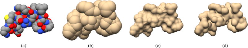
(a) Van der Waals surface; (b) SAS surface; (c) SES surface; (d) Gaussian surface. Images generated with UCSF Chimera [PGH*04] for protein 1wbr.

Figure 2.

Taxonomy of geometry-based methods.

2. Background

There has been considerable work on cavity detection for molecules. This is especially relevant for molecular docking and related problems. A molecule is considered to be an orderly grouping of atoms bound by favorable chemical connections [JKSS96, WM97]. In particular, the family of biomolecules spans the building blocks of living organisms. This family includes large macromolecules, namely proteins, polysaccharides, lipids, nucleic acids, and small molecules (e.g., primary metabolites and secondary metabolites). In this paper, we are interested in proteins and their cavities, where their interactions with ligands usually take place.

2.1. Proteins

Proteins constitute about twenty percent of the human body, and play a crucial role in most biological processes. Amino acids are the building blocks that make up proteins [Whi05]. In summary terms, a protein can be understood at four distinct structural levels [AJL*07]. The primary structure of a protein is given by its sequence (or chain) of amino acids. The secondary structure of a protein comprises amino acid subsequences that exhibit a specific structural regularity. These secondary regular structures are known as alpha-helices (alpha-helixes) and beta-pleated sheets (beta-sheets). Alternatively, the secondary structure can be defined using the regularity of backbone dihedral angles of amino acid residues. The tertiary structure denotes the geometric shape of a given protein, i.e., it refers to the folding of the whole protein chain (including the secondary structures) into its final 3-dimensional shape. Recall that it is the protein folding that makes the protein acquire its functional shape or conformation. Also, many proteins have two or more polypeptide chains or tertiary structures that are held together by the same non-covalent forces as those of tertiary structures, i.e., many proteins can fold into a quaternary structure, resulting in a protein complex.

2.2. Protein Surfaces

Taking into consideration that proteins fold in an aqueous medium, i.e., soluble biomolecules adopt their stable conformation in water (hydrophobic effect) [Sim03], we can think of protein cavities as recesses on a protein surface where water can enter and stay for some time. Therefore, detecting protein cavities depends on features found on the protein surface.

In the literature, we find many mathematical formulations of protein surfaces, namely: van der Waals surfaces (vdW), solvent-excluded surfaces (SES), solvent-accessible surfaces (SAS), and Gaussian surfaces, as illustrated in Fig. 1. For modeling purposes, atoms are often conceptualized as hard spheres, but that is not true because their electronic fields partially overlap within a molecule (e.g., a protein). The van der Waals surface is given by the surface of the union of such atomic spheres [LR71] [Whi97], as shown in Fig. 1(a).

Initially proposed by Lee and Richards [LR71], solvent-accessible surface (SAS) was introduced to model the molecular hydrophobic effect using the vdW surface plus a probe sphere of radius 1.4 Å featuring the water molecule. SAS is the surface generated by tracing the center of the water probe sphere rolling on the vdW surface. In mathematical terms, SAS is also defined as the surface of the union of atomic spheres, but with their radii increased by 1.4 Å. Obviously, SAS is bulkier than van der Waals surface, because the water is taken into account on the molecule, as shown in Fig. 1(b).

Solvent-excluded surface (SES) was introduced by Richards [Ric77] (see Fig. 1(c)), and also uses the rolling probe sphere as SAS, i.e., the probe sphere featuring the water molecule rolls on the vdW surface. SES consists of two parts, the contact surface, and the reentrant surface. The contact surface comprises disconnected patches of the vdW surface that enters in contact with the probe, while the reentrant surface is made up of disconnected patches resulting from the interior-facing part of the probe when it enters simultaneously in contact with two or more atoms. SES is the union of these contact and reentrant patches, resulting in a connected surface.

Gaussian surface is an analytical formulation for molecular surfaces that results from summing up Gaussian functions representing the electronic density fields of atoms that form a molecule [Bli82] (see Fig. 1(d)). The Gaussian surface is smooth because the subsidiary functions decay smoothly to zero with the distance to each atom center.

It is clear that cavity detection algorithms usually start with the reading of the set of atoms in memory, i.e., they inherently use the vdW surface. But, as explained throughout the paper, there is a trend to use analytical surfaces like SES and Gaussian surfaces to detect cavities using geometric properties as of differential geometry, as is usual in segmentation techniques studied in computer graphics [PTRV12] [DG17].

2.3. Protein Cavities

Seemingly, there is no consensus about the definition of cavity, neither about the classification of cavities. Terms such as cavity, pocket, channel, tunnel, void, and cleft are often used in a slightly different way, or even not being defined at all. Some authors describe a pocket as a non-flat and concave molecular surface feature [LJ06, HSAH*09, PSM*10, CS10, GS13], so that pockets and cavities are used interchangeably. Other authors define a cavity as an inner region inside the molecular surface [HRB97, BHH*10, VG10, OMV11, KLKK16], which may lead to the idea that a cavity is a void. It is also observed in the literature that there is an unclear distinction between tunnels and channels [POB*06, OFH*14, PEG*14]. In fact, a formal mathematical definition of protein cavity remains absent in the literature [OFH*14].

How can we define a protein cavity? Informally, we can say that a cavity is a concavity on the protein surface. This leads us to put the theory of convexity in the context of geometric cavity detection methods. Apart its generality, the advantage of using the mathematical theory of convexity [Lay82] is that it provides a formal definition of protein cavity, as follows:

A cavity is a connected component of the complement space of the protein inside its convex hull.

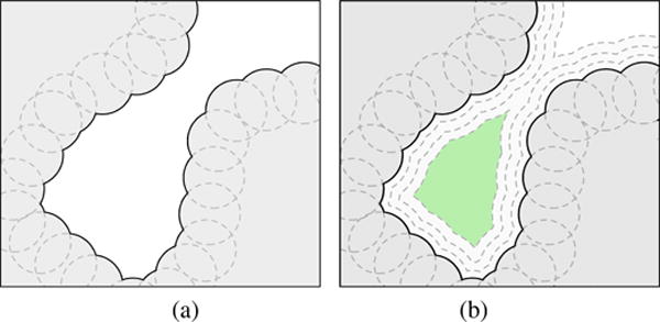
Note that the concept of connected component is topological, and has to do with the first Betti number β₀ (the number of connected components) of such complement space [Hat02]. Looking at the protein itself as a shape in 3D, we know that its connected components, channels, and voids correspond to Betti numbers β_i (i = 0,1,2) in 3D. It is clear that these channels and voids belong the complement space. The remaining connected components of the complement space are pockets. In short, we can breakdown cavities into three classes: pockets, channels, and voids (see Fig. 3).

Figure 3.

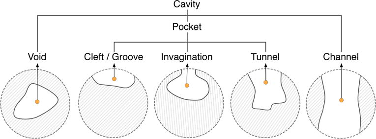
Types of cavities.

The detection of cavities is mostly based on the hydrophobic effect of water on the protein surface; it is assumed that the water molecule is approximately a ball of 1.4 Å of radius. Nevertheless, some channels do not control the flow of water molecules; for example, ion channels control the flow of ions. But, in general, cavities are assumed to be located where the water molecule gets in without slipping on the surface. A major problem with detection of protein cavities has to do with delineating the boundary of each cavity on the protein surface, which consists of zero or more surface contours, called mouth openings. In this sense, a cavity refers to a m-ary cavity, with $m\in \text{ℕ}$ standing for the number of mouth openings to the outside; for example, a void is a 0-ary cavity, i.e., a cavity without mouth openings, a pocket is a 1-ary cavity with a single mouth, while a channel is 2-ary cavity. Note that, from topology’s point of view, a m-ary cavity (m ≥ 3) is a set of m − 1 2-ary cavities of the protein in 3D, which is nothing more than the first Betti number, i.e., β₁ = m − 1. Some of these cavities play an important role in the function of proteins because they are the suitable sites for binding of ligands [GS13].

Summing up, a protein in 3D may only possess three types of cavities: pockets (0-ary cavities), channels (1-ary cavities), and voids (2-ary cavities). Pockets include clefts, grooves, invaginations, and tunnels. A pocket may have zero or more chambers without direct contact with the outside, though they are reachable from outside through a tunnel. Clefts and grooves have no chambers nor tunnels. An invagination is a pocket with a single chamber and no tunnel. A tunnel is a pocket without chambers. As shown in Fig. 4, a pocket can be made of recesses, tunnels, and chambers. Similarly, channels and voids may also possess recesses, tunnels, and chambers.

Figure 4.

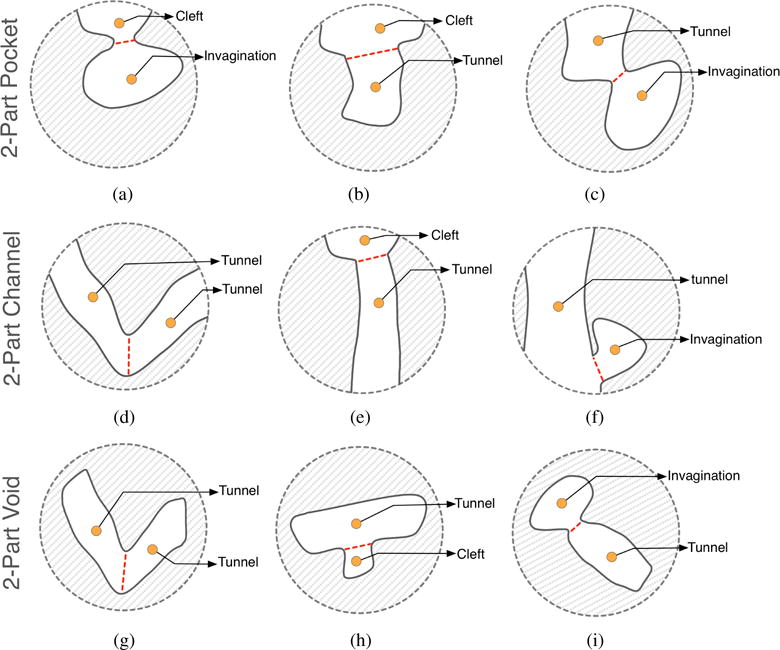
Hierarchical 2-part pocket, channel, and void examples. (a) A pocket composed by a cleft and a invagination; (b) A pocket composed by a cleft and a tunnel; (c) A pocket composed by a tunnel and a invagination; (d) A channel composed by two tunnels; (e) A channel composed by a cleft and a tunnel; (f) A channel composed by a tunnel and a invagination; (g) A void composed by two tunnels; (h) A void composed by a tunnel and a cleft; (i) A void composed by a invagination and a tunnel.

3. Sphere-Based Algorithms

Sphere-based algorithms are based on the concept of probe sphere.

3.1. Kuntz et al.’s method

The first sphere-based method was proposed by Kuntz et. al. [KBO*82], though in the context of geometric docking between a macromolecule and ligands. In fact, the receptor and the ligand are both represented as SES. The cavities of the receptor are filled with probe spheres, and the ligand itself is filled by probe spheres in both cases tangent to the surface points. Then, shape matching operations between the ligand and the receptor probe spheres are approximated under rigid transformations of the ligand. Furthermore, the overlap is evaluated to detect cavities that fit with the ligand. Note that the SES is given as a set of surface points with normals. For further details about probes and receptor-ligand matching, the reader is referred to [KBO*82]. Indeed, the most important aspect of this method is that it is the first method based on the geometry of the ligand.

3.2. HOLE

This method is specialized in tracking channels or holes through proteins [SGW93] [SNW*96]. It requires that the user indicates the seed point inside the channel and vector that represents the direction of the channel approximately. A probe sphere is then centered at the seed point without overlapping the atoms bordering the channel. Then, the probe sphere is moved along the channel, with its radius being adjusted using the Monte Carlo simulated annealing procedure [MRR*53] [KJV83]. Similar to Kuntz et al.’s method, HOLE utilizes large probe spheres of 5 Å radius as stopgap or delimiter of channels.

3.3. SURFNET

SURFNET proposed by Laskowski [Las95] is similar to the method proposed by Kuntz et. al. [KBO*82]. Therefore, its leading idea is also to fill in cavities with probe spheres of varying sizes. However, it differs from Kuntz et al.’s method in the computation of probe spheres. Basically, for every pair of relevant atoms, we place a probe sphere centered at the midpoint of their atomic centers. Then the radius of the probe sphere is adjusted to guarantee that it does not overlap with any neighboring atoms, as illustrated in Fig. 5.

Figure 5.

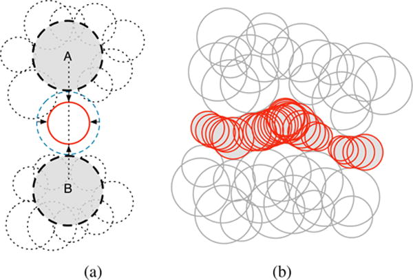
Detecting cavities through SURFNET: (a) Each probe sphere is placed at the midpoint of a pair of atoms (A,B) but, if such probe sphere overlaps at least an atom (dashed spheres), its radius has to be reduced until it just has a tangential contact with the overlapped atom; (b) all probe spheres placed into cavity after considering all pairs of atoms and the surface enclosing of the cavity (pictures taken and modified from [Las95]).

3.4. PASS

PASS (Putative Active Sites with Spheres) is another sphere-based algorithm [BS00]. Cavity filling with probe spheres is carried out in layers, based on three-point Connolly-like sphere geometry [Con83]. That is, the placement of probe spheres of the first layer is performed by looping over triplets of overlapping protein atoms, computing then the three locations at which a probe sphere is tangential to such atoms, as shown in Fig. 6(a). The first layer on the surface consists of probes with radius of 1.8 Å for protein without hydrogen atoms; this radius is 1.5 Å if the hydrogen atoms are taken into account. The subsequent layers accrete probes with 0.7 Å of radius.

Figure 6.

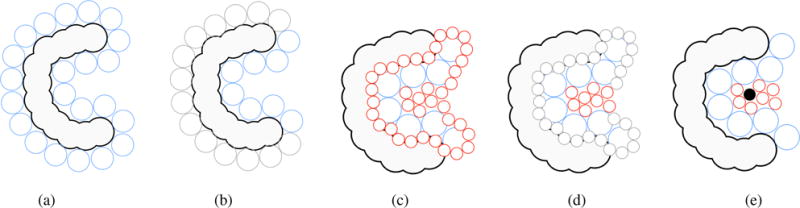
Detecting cavities through PASS: (a) coating the molecular surface with the initial layer of probe spheres (blue spheres) - Probe spheres are tangentially placed to three atoms of the molecular surface; (b) probes of the initial layer (blue spheres) are filtered; they are removed from the initial layer if (i) overlap with any atom belonging to the protein surface, (ii) are in contact with any previous placed probes, and (iii) is at some extend less buried than other probes. In (b) a set of blue spheres, now represented as larger gray spheres, were removed because of (i); (c) more layers are added to the previous layer (red spheres); (d) spheres, as in (b), are filtered until we find an accretion layer that does not contain new probes (i.e. all probes were removed by the set of filters); In (d) a set of red spheres, now represented as smaller gray spheres, were removed because of (i) and (ii). The only remaining set of red spheres are those considered to be more buried on the molecular surface; (e) for each probe, its weight (PW) is computed and the active site point (black sphere) is identified in the cluster (pictures inspired in [WPS07] and [BS00]).

The retained probes must satisfy three conditions: (i) they cannot overlap any atom (see counterexample red probes Fig. 6(c)); (ii) they cannot overlap with one another (see some counterexample red probes Fig. 6(c)); (iii) the burial threshold of each probe must be greater that 55 atoms for hydrogen-free proteins and 75 for proteins with hydrogen atoms; these threshold values were obtained empirically. The buriedness of a probe is determined by the number of protein atoms that lie within an empirical radius of 8 Å, i.e., each probe is given a burial count.

After the accretion and filtering steps (see Fig. 6), it remains to determine the active site points (ASP) of pockets, a single ASP per pocket. So, an ASP represents a potential binding site for a ligand. The ASP of each pocket is determined by identifying the central probe of the corresponding cluster of probe spheres with higher weight (also called probe weight), which depends on the burial count. See Brady and Stouten [BS00] for further details.

3.5. PHECOM

PHECOM (Probe-based HECOMi finder) is yet another sphere-based algorithm and was developed by Kawabata and Go [KG07]. Similar to PASS, it also uses the three-point Connolly-like sphere geometry (i.e. placing a sphere tangential to three atoms of the protein, see Connolly [Con83] for more details) to coat the protein with a set of small probe spheres; the radius of each small probe sphere was set to 1.87 Å, which corresponds to the size of a single methyl group (−CH₃), as illustrated in Fig. 7(a). Additionally, PHECOM also produces a coating of the protein with large probe spheres, so that one removes small probe spheres that overlap with the large probe spheres, as shown in Fig. 7(b). Doing so, one considers that a cavity is an empty space into which a small probe sphere gets in, but not a large probe sphere; for example, this is shown in Fig. 7(c), where small probe spheres (in gray) overlap, indicating the location of a cavity. Note that the probe spheres are allowed to overlap with each other, but not with protein atoms.

Figure 7.

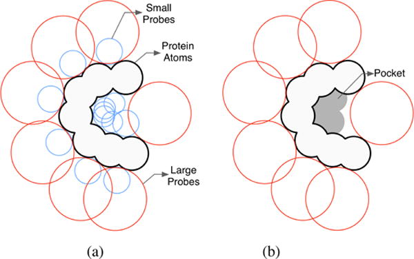
Detecting cavities through PHECOM: (a) small and large probes are placed on the van der Waals surface; (b) small probes that overlap with the large ones are removed - The remaining set of small probes forms the pocket (taken and modified from [KG07]).

3.6. dPredgeo

dPredgeo was developed by Schneider and Zacharias [SZ12]. It is similar to PHECOM because it also uses rolling probes. More specifically, it uses two types of probes with fixed radii. The first probe is 1.4 Å radius and approximates the water molecule, which rolls on the vdW surface of the protein. This rolling procedure of probes reduces itself to the placement of probes on the protein surface according to the principle of three-point geometry mentioned above. The same rolling procedure applies to set of larger probes with 4.5 Å of radius. As for PHECOM, these large probes solve the ambiguity problem that stems from the lack of a cavity stopgap. Then, one discards the small probes overlapping with large probes. Cavities are identified by clusters of the remaining small probes on the protein surface.

3.7. Sphere-Based Methods: Discussion

Table 1 summarizes the characteristics of sphere-based methods in the detection of cavities on protein surfaces. In this regard, we note the following:

• Molecular Surfaces. Sphere-based methods use the set of atoms (SA) —and thus the van der Waals surface indirectly— of each protein as the basis to identify cavities on the protein surface. The first three methods (Kuntz et al., HOLE, and SURFNET) use two-point sphere geometry, while the last three methods (PASS, PHECOM, and dPredgeo) use tree-point Connolly-like sphere geometry [Con83].

• Limitations. One of the main problems of cavity detection methods has to do with automatically finding and delineating cavity boundaries, also called mouth openings, without ambiguity. But, unlike most sphere-based methods, HOLE requires the user provides a seed point inside each channel to start filling it with probe spheres. This means that, unlike most sphere-based methods, HOLE is not capable of determining cavities in an automated manner, i.e., it uses user-assisted cavity localization (UACL). Note that HOLE has been designed only to identify channels.

  In general, sphere-based methods do not suffer from the problem of mouth-opening ambiguity (MOA). Kuntz et al., HOLE, and SURFNET use varying-radius probes (1.4 Å minimum) to fill cavities, though HOLE has been designed only to identify channels. This filling process stops when the probe sphere radius exceeds 5 Å, which works as the stopgap of the cavity; consequently, we can then delineate the corresponding mouth opening. Nevertheless, SURFNET does not utilize large probe spheres as stopgaps of cavities, because the placement of probe spheres in the empty space between pairs of atoms makes such large probes unnecessary.

  The remaining three methods (PASS, PHECOM, and dPredgeo) use two constant-radius probes, a small probe (about 1.4 Å radius) and a large probe (with a radius greater than or equal 4 Å). These methods follow the principle that a cavity is a site where the small probe gets in, but the large probe does not. As noted above, large probe spheres can work as stopgaps (or delimiters) of cavities, so eliminating the mouth-opening ambiguity. However, these large probes are unnecessary for voids because every single void has no mouth opening.

• Cavities. In general, sphere-based methods are capable of detecting any cavity (see Table 1). This is so because these methods are capable of not only filling cavities with probe spheres but also to stop such a filling process. SURFNET utilizes a technique for bracketing probes in the empty space between every atom-atom pair, while PASS takes advantage of the concept of burial threshold; the remaining four methods use large probe spheres as stopgaps of cavities.

Table 1.

Sphere-based methods.

Methods	Reference	Molecular Surfaces	Limitations	Cavities
		SA/vdW	UACL	Pockets			Channels	Voids
				Clefts / Grooves	Invaginations	Tunnels
Kuntz et. al.	[KBO*82]	●		●	●	●	●	●
HOLE	[SGW93]	●	●			●	●
SURFNET	[Las95]	●		●	●	●	●	●
PASS	[BS00]	●		●	●	●	●	●
PHECOM	[KG07]	●		●	●	●	●	●
dPredgeo	[SZ12]	●		●	●	●	●	●

Abbreviations: SA/vdW: set of atoms / van der Waals surface; UACL: user-assisted cavity location.

In the future, one might exploit the concept of mutual visibility for surface atoms as a way to further speed up sphere-based methods, making redundant the usage of empirically large probe spheres as stopgaps of cavities. Note that these large empirical probes work well for small and medium size cavities, but not for shallow cavities, i.e. sphere-based methods have problems with the identification of shallow cavities. In a way, such mutual visibility technique may be seen as a faster follow-up of SURFNET. Another way of improving the identification of cavities would be to consider the detection of n-part cavities.

4. Grid-based algorithms

Grid-based methods are characterized by the following: (i) they use an axis-aligned 3D dimensional lattice; (ii) they use a density map (i.e., a scalar field) so that each grid node is usually assigned an integer value, which gives rise to an integer grid map. Then, one uses some voxel clustering to collect relevant empty voxels into cavities.

4.1. CAVITY SEARCH

This method was introduced by Ho and Marshall [HM90]. It uses a slice-to-slice filling procedure for each cavity in a single direction, which is perpendicular to slices, to isolate and delineate the boundary of such cavity, thereby producing a cast (i.e., a cumulative set of slices of grid nodes or voxels) of the cavity. After filling in a slice of a given cavity using a two-dimensional flood fill algorithm, we have to step forward to the next slice, repeating the filling procedure. However, this procedure suffers from two shortcomings. First, it requires a starting seed node for each cavity, which is supposedly supplied by the user. Second, the filling of a cavity may go wrong if the slice of voxels extends out of the cavity, as a consequence of the non-closedness of the boundary of the cavity.

Summing up, the detection of a cavity is done per slice of the grid, but one only considers slices that are transverse to cavities, i.e., the cavity inside a slice is delimited all around. The main drawback of this method is that it fails to detect clefts/grooves when the slices do not meet the incomplete boundary of the cavity, although voids are always identified correctly. Invaginations, tunnels, and channels may also not be correctly identified for the same reason.

4.2. POCKET

POCKET was proposed by Levitt and Banaszak [LB92]. Its leading idea is to search for cavities along one or more directions. As a grid-based algorithm, it firstly maps the molecule onto an axis-aligned grid of equally-spaced points. The detection of cavities is carried out by scanning them along with x, y, and z axes. The x-axis scan is repeatedly done for all y and z values, starting on those grid points belonging to the leftmost plane of the 3D grid where x is minimum, i.e., x = x_min, as illustrated in Fig. 8(a)–(b); analogous procedure applies to y-axis scans and z-axis scans.

Figure 8.

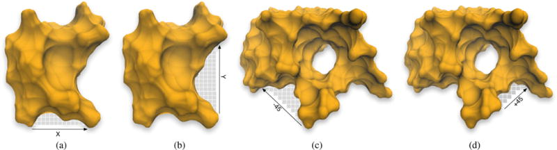
Detecting cavities through POCKET (see [LB92]): (a) in the x-direction; (b) in the y-direction. Detecting cavities through LIGSITE (see [HRB97]): (c) in the −45°-direction; (d) in the +45°-direction.

A grid is used to calculate a density map for a given protein. Initially, all grid points are set to a density value of 0. Then, for each voxel on the vdW surface of the protein, one has to check whether there is or not another boundary voxel along the x, y, and z directions outwards the surface. If so, all the voxels between those two boundary voxels are set to a density value 1. In this way, we end up having voxels with density value 1 that are gathered into separate clusters of value-1 voxels, a cluster per cavity.

Unlike CAVITY SEARCH, this method works in an automated manner, i.e., it does not require the user assistance to indicate the seed node of each cavity. However, the identification of cavities still depends on the alignment of the protein about the coordinate system of the grid [LJ06]. For example, a counterclockwise rotation of the molecule shown in Fig. 8(a) by 45°, makes its bottom cavity undetectable along the x direction. That is, POCKET is protein-orientation sensitive (POS), and this is particularly noticeable for clefts/grooves.

4.3. LIGSITE

To mitigate this ambiguity problem that results from aligning a protein in grid coordinate system, Hendlich et al. [HRB97] developed a more sophisticated scanning method, which was implemented in LIGSITE. In addition to the three scans along x, y, and z, they used four more scans along the Cartesian cubic diagonals [LJ06], in a total of seven directions, in the attempt of making the identification of cavities less dependent on the orientation of the protein embedded in the 3D grid, as illustrated in Fig. 8(c)–(d). These seven directions correspond to 14 oriented directions; for example, x direction corresponds to two oriented directions, x and −x. In practice, if we think in terms of grid cubes neighboring a given grid cube, these 14 oriented directions are those defined by 14 out of 26 grid cubes surrounding a given cube. As explained further ahead, Li et al. [LTA*08] extended the number of scanning directions to those 26 oriented directions in VisGrid.

4.4. Exner et al.’s method

Exner et al. [EKMB98] proposed a grid-based method similar to POCKET [LB92] to predict cavities in molecular structures, in the sense that it also uses negative and positive x, y, and z directions for scanning cavities of a given protein. The grid spacing is set to 0.5 Å. The grid points inside protein atoms are labeled as ‘in’ points, while those outside such atoms are labeled as ‘out’ points.

Exner et al.’s method distinguishes itself from other grid-based methods because the bracketing strategy for each ‘out’ grid is confined to a distance of 12 Å, i.e., to a ball of 12 Å radius centered at each ‘out’ grid point. That is, an ‘out’ grid point is defined as a cavity point if it is bracketed by two ‘in’ grid points along at least two Cartesian axes. This means that grooves are not detected at all.

Then, those ‘out’ grid points that are cavity points are combined to form clusters or cavities. Exner et al.’s method uses two cellular logic operations, known as contraction and expansion, to build up such clusters [Del92].

4.5. PocketPicker

An algorithm similar to POCKET and LIGSITE was developed by Weisel et al. [WPS07] and is called PocketPicker. The main difference between PocketPicker and its predecessors is that the scanning is performed along 30 directions equally distributed on a sphere [SK97]. A scan is performed for a probe sphere centered at each grid point beyond the protein surface (i.e., vdW surface) and falling short of an outer surface that does not exceed a maximal distance of 4.5 Å relative to the protein surface (Figure 9). Grid points inside the protein surface and outside the outer surface are not considered in the computations.

Figure 9.

Detecting cavities using PocketPicker [WPS07]: (a) Group of grid points in the outer surface (green squares) inside the protein surface (gray squares) and outside of the outer surface (white squares); (b) Cluster of grid points that represent cavity regions (pictures taken and modified from [WPS07]).

The solvent accessibility of a grid probe along its 30 directions determines the buriedness of each grid point. Whenever a vector defined by one of these directions hits a protein atom, the buriedness index of the grid point increases by one. After calculating the buriedness index for each grid point between the protein surface and the outer surface, it remains to cluster the grid points into pockets. A pocket consists of connected grid points with a buriedness index greater than 15 (out of 30 directions), what intuitively indicates that the grid points belong to a concavity of the protein surface. A grid point whose buriedness index is less than 15 is one that is above a convex part of the protein surface. Note that the buriedness index is a discrete measure of the solid angle of Connolly [Con86].

4.6. PocketDepth

PocketDepth is another grid-based algorithm, which was proposed by Kalidas et al. [KC08]. It is similar to POCKET in the sense that it uses six oriented scanning directions for each voxel, each direction per voxel face. Thus, it is also protein-orientation sensitive (POS). Also, it resembles the Travel Depth method (see Section 7.3), provided that its scalar field is set by calculating the depth of each cube’s center of putative cavities within an axis-aligned grid. But, unlike Travel Depth, the depth is counted in an incremental manner, rather than measured (see Eq. (3)), from a grid cube to its neighbors.

The algorithm is as follows. First, all grid cubes are assigned the zero depth and labeled as internal, external or surface. Note that each surface cube defines six axis-aligned vectors. Second, considering only the axis-aligned vectors that go out the surface, and that are blocked by any surface cube on the other side of the surface, the depth of each cube located between two opposite blocking cubes on the surface is incremented by 1. Third, grid cubes with a depth greater than zero are then clustered into cavities regarding their cumulative depth and spatial proximity. The cube clustering is based on the DBSCAN, which is a density-based clustering scheme due to Ester et al. [EKSX96].

4.7. VisGrid

With VisGrid, Li et al. [LTA*08] extended LIGSITE in the sense that it uses the 26 oriented directions defined by the 26 voxels of the first layer around a given voxel, and 98 when the second layer is taken into account. Therefore, the problem of orientation-sensitivity inherent to grid-based methods is rather mitigated. The grid voxel length is set to 0.9 Å. The scalar field associated with the grid considers three integer values for voxels: −1 for voxels inside the protein atoms augmented by 1.4 Å concerning the water molecule radius, 0 for voxels transverse to SAS, and 1 for empty voxels outside SAS, although the SAS does not need to be evaluated. Note that the negative scalar value ascribed to interior voxels allows us to find also protrusions as cavities inside SAS.

4.8. PoreWalker

PoreWalker [PCMT09] is a method specifically designed to identify and describe channels (or pores) in transmembrane proteins. A channel is used as a path for ions or other molecules to cross the membrane. Its center and axis can be defined by the pore-lining residues in the protein structure that the algorithm calculates by taking into account the special geometry of transmembrane proteins, as their structures run approximately perpendicular to the membrane plane, crossing the membrane from one side to another.

First, an initial approximation of the main axis of the channel is obtained by taking the C_α coordinates of the residues and calculating the average vectors of the secondary structure (helices and strands). The protein is then re-oriented so that these secondary structures are mainly perpendicular to the membrane and their averaged center of gravity lies at the reference frame’s origin. Next, the center of the pore is identified by iteratively maximizing the number of detected assumed pore-lining residues, i.e. water-accessible amino acids whose C_α–C_β vector points towards the current pore axis, with the preliminary center and axis of the pore being redefined on each step. The final pore axis is obtained by using an iterative slice-based approach to refine it. The protein structure is mapped onto a 3D grid and then divided into slices of height 1Å, perpendicular to the current pore axis. For each slice, located at different pore heights, a local pore center is identified by the center of the sphere with the maximum radius that the slice can accommodate. These spheres then define a new vector used to align and re-orient the structure.

Finally, the algorithm calculates several pore features and quantitative descriptors, such as the diameter profiles and position of pore centers at different heights along the channel, the atoms and corresponding residues lining the channel walls, and the size, shape, and regularity of the channel cavity.

4.9. DoGSite

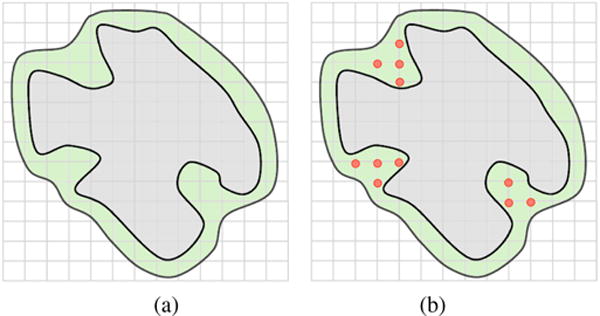
DoGSite was introduced by Volkamer et al. [VGGR10], and is based on the concept of DoG (Difference of Gaussian) [GW07], borrowed from image processing and analysis. The difference is that now we apply a DoG to a 3D grid instead of a 2D image. Grid points are ascribed either the value 0 for points outside the vdW surface or the value 1 for points inside or on the surface. Unlike most cavity detection methods, DoGSite is capable of structuring cavities into subcavities, resulting in a more detailed shape description of putative binding sites.

DoGSite was developed from the leading idea that active sites quite often possess invaginations as large as that they are capable of accommodating one or more heavy atoms. When a 3D DoG filter is applied to a grid representation of the protein, such invaginations can be identified because it determines where are spherically shaped structures in the grid, known as DoG cores. These cores correspond to subcavities that are then gathered into cavities.

4.10. VICE

VICE (Vectorial Identification of Cavity Extents) is another grid-based method, which was developed by Tripathi and Kellogg [TK10]. Similar to other grid-based methods, VICE discards grid points that fall inside the protein surface (e.g., vdW surface). Only the grid points that fall outside the protein surface are assigned a score according to a buriedness-like metric.

Similar to POCKET, VICE uses an integer (Boolean) grid, but the values 0 and 1 assigned to grid points have a distinct meaning. The value 0 is assigned to every single grid point inside an atom; otherwise, its value is set to 1. VICE uses an integer density map to define the scan directions through integer arithmetic vectors as a way of speeding up the computations associated with the grid. It is clear that the grid points outside the protein potentially are cavity points, and this leads us to the ambiguity problem of cavity bounds. Each outside grid point is subject to a search procedure to determine whether it belongs to a cavity or not.

The decision is based on a discrete variant of the Connolly function, in a way similar to that one of PocketPicker. Basically, one considers a set of eight 2D vectors (1,0), (1,1), (0,1), (−1,1), (−1,0), (−1,−1), (0,−1), and (1, −1) from each grid point to its eight neighbouring points in the same axis-aligned plane (e.g., parallel to the XY plane), and calculate the rate of blocked vectors to the total number of vectors starting at such grid point. A blocked vector is defined as any vector that hits the molecular surface (or atom); otherwise, it is a clear vector. Such a rate has a nominal cutoff value given by 0.5, which sets the line between the convexity and the concavity. A rate clearly above 0.5 denotes the presence of a putative cavity, while a rate noticeably under 0.5 means that the grid point is close a convex region of protein surface or it is far away from the protein surface. It happens that a few grid points, mostly those close to the cavity mouth, remain ambiguous because the rate varies in the range [0.5 − 0.05, 0.5 + 0.05]; in this case, one uses a supplementary set of 2D vectors given by (2,1), (1,2), (−1,2), (−2,1), (−2,−1), (−1,−2), (1,−2), and (2,−1) for disambiguation purposes.

4.11. Phillips et al. method

This method was proposed by Phillips et al. [PGD*10]. It is based on ray casting, as known from computer graphics, with the difference that rays are parallel to each other in z direction. This technique utilizes a ray passing through the centers of voxels of an axis-aligned 3D grid hosting the protein. As usual in ray casting, rays are not blocked by the protein, so that we end up having door-in and door-out points on the molecular surface (e.g., vdW surface) for each ray. These intersection points between rays and the molecular surface are carried out as usual in computer graphics. In the end, we have only to collect those voxels outside the surface that are traversed by door-out-door-in ray segments. Unfortunately, and similar to CAVITY SEARCH and other methods with a small number of scanning directions, this technique may miss cavities other than voids.

4.12. Grid-Based Methods: Discussion

Grid-based methods are built upon three entities: the set of atoms (SA) of a given protein, an axis-aligned grid, and a scalar field. The scalar field is either boolean or integer. The key idea of these methods is the one of blocking oriented directions or visibility vectors from each voxel. A brief glance at Table 2 shows us grid-based methods enjoy the following characteristics:

• Molecular Surfaces. As shown in Table 2, and similar to sphere-based methods, grid-based methods mostly rely on the set of atoms (SA). Atoms allow us to distinguish the grid nodes inside the protein (or inside of atoms) from those lying outside it.

• Limitations. We have identified two main limitations with grid-based methods. The first has to do with grid-spacing sensitivity (GSS). A distinct grid voxel length may result in finding distinct cavities for the same protein [OFH*14], as well as a different number of cavities. Clearly, this has not only a significant impact on the accuracy of a given grid-based method but also on its performance regarding memory space and time complexity. In fact, a grid with smaller voxels implies more memory space consumption and poorer time performance, in particular for voxel length less than 1.0 Å. To mitigate the problem of grid-spacing sensitivity, one has to find a way of automatically adjusting and calculating the appropriate voxel length. With the exception of DoGSite, no other method can automatically adjust the voxel length to the size of a given protein regarding the number and density of atoms. Larger proteins should lead to longer voxel length [VGGR10], and thus a less number of voxels, as well as an increasing of time performance. Recall that the time complexity of any algorithm based on a 3D grid is cubic unless one uses parallel computing [DG17].

  The second limitation concerns protein-orientation sensitivity (POS). This means that a distinct orientation of the protein within the grid may result in finding a distinct set of cavities on the same protein surface [BAM*14]. That is, grid-based methods are not rotation-invariant; their accuracy depends on rotations of a given protein in 3D space. Using multiple scanning directions is a way of mitigating this problem.

  Note that the problem concerning protein orientation can be solved since we can determine the boundary of each cavity, i.e., the problem of delineating the cavity ceiling [OFH*14]. As shown in Table 2, most grid-based methods have no difficulties in finding cavity mouth openings from the blocking technique of scanning directions.

• Cavities. With the exception of CAVITY SEARCH, grid-based methods identify cavities in an automated manner. Besides, only POCKET and its follow-up method called PocketDepth may miss clefts/grooves because of the small number of scanning directions they use in the detection of cavities.

Table 2.

Grid-based methods.

Methods	Reference	Molecular Surfaces			Limitations				Cavities
		SA/vdW	SES	SAS	GSS	POS	MOA	UACL	Pockets			Channels	Voids
									Clefts / Grooves	Invaginations	Tunnels
CavitySearch	[HM90]	●			●	●	●	●					●
POCKET	[LB92]	●			●	●	●			●	●	●	●
LIGSITE	[HRB97]	●			●				●	●	●	●	●
Exner et al.	[EKMB98]	●			●					●	●	●	●
PocketPicker	[WPS07]	●			●				●	●	●	●	●
PocketDepth	[KC08]	●			●	●	●			●	●	●	●
VisGrid	[LTA*08]	●		●	●				●	●	●	●	●
PoreWalker	[PCMT09]	●			●						●	●
VICE	[TK10]	●			●				●	●	●	●	●
DoGSite	[VGGR10]	●							●	●	●	●	●
Phillips et. al.	[PGD*10]	●	●		●	●	●						●

Abbreviations: SA/vdW: set of atoms / van der Waals surface; SES: solvent-excluded-surface; SAS: solvent-accessible surface. GSS: grid-spacing sensitivity; POS: protein-orientation sensitivity; MOA: mouth-opening ambiguity; UACL: user-assisted cavity location.

At last, with the exception of DoGSite, these methods were not designed to identify n-part cavities in a structured manner, i.e., each n-part cavity is identified as a whole, not in parts or subcavities.

5. Grid-and-Sphere Based Methods

Grid-and-sphere based methods combine the advantages of both grid- and sphere-based methods. Similar to grid-based methods, they also sustain themselves on a scalar field defined at every single grid point. Additionally, they mostly use large probe spheres rolling on the vdW surface, which have the function of delimiting cavities between the probe-generated surface and the molecular surface. This solves the problem of ambiguity that stems from the necessity of identifying cavities and their stopgaps (or mouth openings). The identification of a cavity’s stopgap is known as the cavity ceiling problem. As noted by Oliveira et al. [OFH*14], the cavity ceiling problem can be controlled using customizable probe sizes. Consequently, grid-and-sphere based methods are not orientation-sensitive.

5.1. VOIDOO

VOIDOO is a grid-and-sphere based method proposed by Kleywegt and Jones [KJ94]. It was thought of to only identify voids and invaginations using a process named atom fattening. Unlike a void, an invagination is exposed to the outside of the protein, but it can be closed off by increasing the atomic radii, i.e., an invagination becomes a void using such process of atom fattening. Additionally, an invagination may possess one or more mouth openings, so that channels are also identified using VOIDOO. Unfortunately, wide and shallow clefts/grooves cannot be detected in this manner. Note that the atoms and probes of gradually increasing radii are concentric. This process is shown in Fig 10.

Figure 10.

Detecting cavities using VOIDOO [KJ94]: (a) Region of the protein with atoms having the normal van der Waals radii; (b) The increase of the atomic radii of the atoms encloses a cavity (green zone). This process of atom fattening allows a well delineation of the void (pictures taken and modified from [KJ94]).

This method starts by mapping the protein onto a 3D grid with the following characteristics: (i) grid spacing of 0.5 to 1.0 Å; (ii) grid nodes ascribed with the value 0. The second step consists in labeling all grid points inside protein’s atoms (i.e., vdW surface) as 1. The third step carries out the labeling of those grid points that gradually are caught between the vdW surface and the SAS-like outer surface under the process of atom fattening. This process stops as soon as the invagination turns into a void.

5.2. HOLLOW

HOLLOW is a grid-and-sphere method proposed by Ho and Gruswitz [HG08]. HOLLOW uses a grid with a spacing of 0.5 Å, and probe spheres (called dummy atoms) of 1.4 Å radius. Unlike sphere-based methods, which place probe spheres tangential to three atoms of the protein, here each probe is centered at a grid point.

Then, those dummy atoms overlapping atoms of the molecule are thrown away from the grid. Also, dummy atoms located outside the envelope of the protein are removed. In the same manner, the remaining dummy atoms within each cavity are eliminated under the condition that the total volume of each cavity remains the same. The envelope of the molecule is defined by the process of rolling a large probe sphere of 8.0 Å on the surface atoms. Consequently, all cavities of the molecule are identified by HOLLOW, but this evidently depends on the grid spacing.

5.3. POCASA

POCASA (Pocket-Cavity Search Application) includes a sphere-based grid algorithm, called Roll, which was designed and developed by Yu et al. [YZTY10]. The scalar field is boolean, so that grid points inside the protein are assigned the value of 1 (i.e., occupied grid points), while grid points outside the protein take on the value 0 (i.e., free grid points).

Roll makes use of a large probe sphere of a varying radius much greater than 1.4 Å, which rolls on the protein surface, being the rolling direction controlled by the inner border tracing algorithm borrowed from image analysis and processing [SHB16]. Nevertheless, the size of the probe sphere may vary to identify cavities of distinct sizes. The crust-like surface generated by the probe works as a second envelope of the protein and is called probe surface. The leading idea is to identify cavities as the loci consisting of free grid points or voxels between the protein’s vdW surface and the probe surface. In practice, the probe surface is not generated, being enough to consider as cavity voxels the free voxels outside the protein that are not touched by the probe. Obviously, the voxels beyond the probe are discarded straight away.

5.4. McVol

McVol method was proposed by Till and Ullmann [TU10] to calculate the volume of molecular structures through a Monte Carlo integration. The molecular volume is used to identify surface clefts and voids. This method takes advantage of four main tools: (i) an axis-aligned grid enclosing the molecule; (ii) the solvent-accessible surface (SAS); (iii) spherical probe rolling on the set of atoms of the molecule, whose radius is desirably equal to the atomic radius of the solvent; (iv) the random placement of points in the grid-discretized domain (i.e., bounding box) enclosing the molecule.

The random placement of points in the domain serves two purposes: the computation of the molecular volume and the identification of voids. In fact, the molecular volume consists of the volume enclosed by the outer surface minus the volumes (voids) enclosed by the inner surfaces. Therefore, the computation of the molecular volume requires identifying the molecular voids. Note that grid-based methods are suited to compute volumes via integration via Monte Carlo techniques. See Till and Ullmann [TU10] for further details. A point that belongs to a void satisfies the following two conditions: (i) its distance to any atom center is less than the vdW radius of such atom plus the rolling probe sphere radius; (ii) its distance to SAS’ closest point is greater than the rolling probe sphere radius.

Identifying surface clefts is inspired by the technique used to identify voids. We define a 3D local box centered at each solvent grid point (i.e., grid point outside the molecule) to determine the percentage of cleft grid points in the local box. If such a percentage is greater than a given threshold, the solvent grid point is marked as cleft, what is equivalent to use a discrete Connolly function. The clustering of solvent grid point into clefts is performed using a breadth-first search (BFS) over the grid.

5.5. GHECOM

GHECOM (grid-based HECOMi finder) is a grid-and-sphere based method due to Kawabata [Kaw10]. It is a follow-up of the sphere-based method, called PHECOM, proposed before by Kawabata any Go [KG07]. Following the principle that probes with different radii capture distinct protein cavities, PHECOM uses the smallest probe whose radius is 1.87 Å, which corresponds to the size of a single methyl group (−CH₃), and a variable size for the large probe that defines not only the cavity ceiling but also the shallowness of the cavity. Besides, this idea is taken to a limit in methods based on α-shapes (see Section 8), where radius-zero probes outputs the van der Waals surface and radius-∞ probes gives rise to the convex hull of a set of atoms.

As Kawabata noted, placing probes on the protein atoms in conformity with the principle of three contacts (i.e., three-point geometry) might fail for proteins with irregular shapes. Besides, computing the minimum inaccessible radius for a set of large probes is very time-consuming. This amounts to computing the optimal α-sphere that defines the ceiling (i.e., stopgaps) for all relevant cavities of a protein (see Section 8).

GHECOM solves these problems by combining spheres with voxels of a 3D grid, together with the theory of mathematical morphology [Mat75] [Ser84]. This theory is used in digital analysis of geometric features in imaging, although it had also been used in the structural analysis of proteins before by the hand of Delaney [Del92] and Masuya and Doi [MD95]. According to Masuya and Doi, given the set X of the union of the atoms of a given protein, pockets can be defined as the result of closing of X by a large probe and opening of X by a small probe; note that closing (●) and opening (○) are two morphological operations. Masuya and Doi also put forward that the SAS and SES can also be defined through morphological operations.

Kawabata’s solution for identifying cavities also uses those morphological operators, which reflect the PHECOM definition of a pocket: “a small probe can enter but a large probe cannot” [Kaw10]. In fact, GHECOM uses the same two operations to define a pocket of X as follows:

$$P_X(L,S)=\left((X•L)\cap X^C\right)\circ S$$ (1)

where L and S stand for the large and small probes, and X^C is the set complement of X. As shown in Fig. 11, the operation (1) produces a pocket as the space outside the protein X (X^C), where the large probe L cannot enter (closing of X by L), but the small probe S can (opening of (X ● L) ∩ X^C by S). So, it was made possible to efficiently calculate multiscale pockets (i.e., deep to shallow pockets), simultaneously, from multiscale spherical probes (i.e., small to large probes). It is noteworthy that the expression (1) simplifies analogous expression advanced by Masuya and Doi, and is valid for both continuous and discrete point sets, i.e., it applies to sets defined in the 3D grid of the domain where the protein resides.

Figure 11.

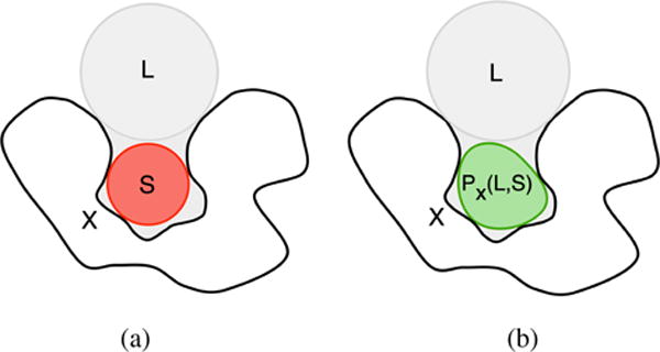
Detecting cavities using GHECOM [Kaw10]: (a) representation of the molecular surface (X), a small probe (S) in a cavity, and a large probe (L) on the protein surface; (b) cavity as given by P_X(L,S).

5.6. 3V

Voss and Gerstein [VG10] introduced the 3V (Voss Volume Voxelator) method. It also uses two probes that roll on the set of atoms of the protein, whose radii can be adjusted relative to their 1.5 and 6 Å default values. These probes define two solvent-excluded surfaces, but these surfaces are not analytically built nor triangulated.

The leading idea is to determine grid points inside the outer surface not accessible to a large probe, as well as grid points inside the inner surface not accessible to a small probe, so cavities result from the difference between the previous two grid point sets. That is, the empty space between the two surfaces is calculated in a discrete manner using a 3D grid of points or voxels. Thus, there is no room for mouth-opening ambiguity (MOA).

5.7. VolArea

VolArea was introduced by Ribeiro et al. [RTC*13]. It also follows the leading idea of mapping a protein onto a 3D grid of voxels, where the cavities are 3D sites that consist of empty voxels located outside the protein. VolArea utilizes the concept of cavity probe sphere that is concentric with every single atom, but whose radius is greater than the vdW radius of its concentric atom. Therefore, similar to VOIDOO (see Section 5.1) and PocketPicket (see Section 4.5), we end up having two surfaces: a vdW surface and an SAS-like surface.

The question is then how to collect the relevant empty voxels of a cavity among all those lying between those surfaces. This is accomplished with the user assistance, who has to first choose the region where to search for a cavity. The user must also set the radius of the cavity probe, which depends on the size and shape of the pocket, cleft or cavity under study.

Then, the cavity is identified from the cluster of empty voxels located inside 3D regions that result from intersecting cavity sphere probes. This means that the voxel length must be much smaller than the radius of any atom. With Volarea, very small cavities are discarded, in particular, those smaller than a hydrogen atom regarding occupied volume.

5.8. KVFinder

More recently, Oliveira et al. [OFH*14] introduced KVFinder, which is another grid-and-sphere based algorithm similar to the one proposed by Voss and Gerstein [VG10]. The scalar field associated with the grid is boolean. This allows them to define every single geometric cavity regarding theory of mathematical morphology [Ser84], as explained below.

The mouth-opening ambiguity problem is approached using two probe spheres: probe-in sphere and probe-out sphere. Only grid points outside the protein are taken into account in the process of detection of cavities. The first sphere is small to guarantee that it fits in most cavities, while the second is larger to guarantee that it does not fit in those cavities. It is clear that we are assuming that these spheres do not overlap the protein surface.

By centering the probe-in sphere at each outer grid point, we easily see that most outer grid points end up being caught by the probe-in sphere; only those grid points of tiny cavities whose size is less than the size of the probe-in sphere are discarded. This concludes the first step of the algorithm. The second step is identical to the first step, with the difference that now one uses the probe-out sphere, instead of the probe-in sphere.

A cavity point is thus every single grid point overlapped by the probe-in sphere which is not overlapped by the probe-out sphere. Note that the probe-in sphere rolling on the protein surface defines a surface that is the SES approximately, while probe-out sphere rolling on the protein surface gives rise to another surface that tends to make a shortcut on the surface, more specifically where the cavities are located. However, these surfaces are not evaluated nor determined analytically. In short, the probe-out sphere solves the mouth-opening ambiguity (MOA) problem that is typical in grid-based algorithms. But, finding a suitable radius for the probe-out is a difficult—not to say impossible—task because the radius depends on the size and shape of each cavity.

5.9. PrinCCes

Recently, a method designated as PrinCCes (Protein internal Channel and Cavity estimation) was proposed by Czirják [Czi15]. The method relies on a three-dimensional grid, whose grid spacing is user-defined and varies between 0.1 and 2.4 Å. Two probe spheres are also employed in the process. A larger probe (with a radius of 1.0 to 10.0 Å of radius) aims at identifying the shell volume (i.e., protein volume plus its cavity volumes), while a smaller probe (with a radius of 0.6 to 5.0 Å of radius) aims at detecting cavity volumes.

This method is quite different from those that place probe spheres in contact with protein’s surface atoms (see, for example, 3V [VG10]). Instead of rolling probe spheres on protein’s surface atoms, both larger and smaller probes are placed at the center of each (surface) atom to collect cavity grid points. In fact, this method relies on a novel algorithm called Find Continuous SubSpace algorithm (FCSS), which decomposes the space between the larger and the smaller probe into distinct cavities.

More specifically, each cavity is delineated by moving a controllable-size probe sphere along the 26 possible directions defined by each cavity grid point and their neighbors, but without colliding with the molecular surface. These movable probes are located in the space between surface atoms and their larger probes.

According to its authors, this method is more faithful to represent the geometric structure of tunnels. That is, it avoids the representation of tunnels as a group of different sized spheres (as seen in CAVER [POB*06] and MolAxis [YFW*08]). Furthermore, the user does not need to provide seed points indicating the direction or location of cavities to detect and delineate cavity zones.

5.10. Grid-and-Sphere-Based Methods: Discussion

Using probes in grid-based methods follows three different techniques. The first is based on atom fattening (originating SAS or SAS-like surfaces), as it the case of VOIDOO, McVol, VolArea, and PrinCCes (see column ‘SAS’ on Table 2). The second takes advantage of the concept of rolling probes of unequal radii on the vdW surface, as in POCASA, McVol, GHECOM, and 3V. The third was only incorporated in KVFinder and consists in placing concentric probes of unequal radii at grid points so that the small probe gets in cavities, but not large probes.

As shown in Table 2, grid-and-sphere-based methods can be characterized as follows:

• Molecular surfaces. As usual, these methods directly use the set of atoms (SA) of a given protein to identify its cavities (see Table 3). Also, and given the hybrid flavor of grid-and-sphere-based methods, they take advantage of three tools: an axis-aligned grid, a scalar field, and probe spheres.

• Limitations. The issue concerning grid-spacing sensitivity (GSS) can be solved since the voxel length is at most (1/2R), with R the radius of the water probe sphere, in conformity with Nyquist theorem [DG15]; otherwise, cavities cannot be properly sampled by empty voxels.

  Protein-orientation sensitivity (POS) is a typical problem in grid-based methods. But, using large probe spheres (approx. 5 Å), we can block cavity entries/exits or mouth openings, solving the POS problem in this manner.

  Mouth-opening ambiguity (MOA) is another issue of grid-based methods, simply because mouth-openings do not block scanning directions. As said above, this problem can be solved using large blocking spheres on the protein surface. With the exception of VolArea, the methods listed in Table 2 resolve the MOA problem, i.e., they are capable of delineating the mouth openings of cavities. This is accomplished at the cost of using probe spheres that isolate cavities from the empty outer space. Let us also mention that only POCASA, GHECOM, and PrinCCes support multiscale probes.

  Therefore, these methods determine protein cavities in an automated manner without the user intervention; the exception is VolArea, which requires the user-assisted cavity localization (UACL).

• Cavities. In general, grid-and-sphere based methods are capable of automatically identifying cavities. Only VolArea needs user’s interactive assistance to identify such cavities (see column ‘UACL’ in Table 3). Nevertheless, VOIDOO may miss shallow cleft/grooves, whereas McVol was designed only for detecting cleft/grooves and voids. At last, among all methods listed in Table 3, only PrinCCes can organize a cavity from its sub-cavities or parts.

Table 3.

Grid-and-sphere-based methods.

Methods	Reference	Molecular Surfaces		Limitations		Cavities
		SA/vdW	SAS	GSS	UACL	Pockets			Channels	Voids
						Clefts/Grooves	Invaginations	Tunnels
VOIDOO	[KJ94]	●	●	●			●	●	●	●
HOLLOW	[HG08]	●		●		●	●	●	●	●
POCASA	[YZTY10]	●		●		●	●	●	●	●
McVol	[TU10]	●	●	●		●				●
GHECOM	[Kaw10]	●		●		●	●	●	●	●
3V	[VG10]	●		●		●	●	●	●	●
Volarea	[RTC*13]	●	●	●	●	●	●	●	●	●
KVFinder	[OFH*14]	●		●		●	●	●	●	●
PrinCCes	[Czi15]	●	●	●		●	●	●	●	●

Abbreviations: SA/vdW: set of atoms / van der Waals surface; SES: solvent-excluded-surface; SAS: solvent-accessible surface. GSS: grid-spacing sensitivity; UACL: user-assisted cavity location.

To summarize, using probe spheres together with grids solves two typical problems of grid-based methods, namely: mouth-opening ambiguity (MOA) and protein-orientation sensitivity (POS). In fact, the use of multi-scale probes allows us to define suitable stopgaps for each cavity.

6. Surface-Based Methods

These methods are based on analysis of geometric properties of the molecular surface [NH06]. Examples of such geometric properties are solid angles [Con86], the surface fractal dimension [PB99], and curvature [NWB*06], so surface cavities look like valleys in the middle of mountain ranges.

6.1. NSA

NSA (Nearest Surface Atom) method was introduced by Del Carpio et al. [DCTS93]. This method starts by sampling the surface of each atom as proposed by Lee and Richards [LR71] for computing the solvent-accessible surface (SAS). Then, one removes the occluded points, i.e., those points inside other atoms (see Lee and Richards [LR71]), so that we end up obtaining a set of points, called free points, which sample the van der Waals surface of the protein. After discarding those occluded points, one calculates the distance between each atom and the center of gravity of the protein. A smaller distance from an atom to protein’s gravity center means that the atom is located at a deeper site in the protein. After finding the nearest surface atom (NSA) from the center of gravity, a cavity is formed by clustering of the nearby surface atoms that are visible to NSA’s free points on the vdW surface (see Fig. 12(a)). The process is repeated while there exists some concavity to detect on the molecular surface (see Fig. 12(b)). The concave regions are the places where the protein cavities are located [DCTS93, LJ06]. However, this method has difficulties in dealing with n-part cavities because it is based on a visibility criterion from the free points of the NSA, i.e., there is space for ambiguity in the identification of cavity mouth openings.

Figure 12.

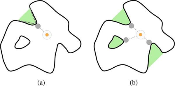
NSA: (a) the gravity centre (in orange) of the protein is displayed together with its nearest surface atom (NSA), from which the cavity (in green) is formed by the clustering of nearby surface atoms that are visible from NSA; (b) the process is repeated while there is some cavity to form on the protein surface (pictures inspired in [LJ06]).

6.2. SCREEN

Nayal and Honig [NH06] proposed a surface-based method, called SCREEN (Surface Cavity REcognition and EvaluatioN). This method generates two molecular surfaces through GRASP [NSH91]. The first surface is the standard SES generated from rolling a solvent probe sphere with 1.4 Å of radius on the van der Waals surface (or set of atoms), here called inner surface. The second surface, called surface envelope, is generated in the same manner, but with a probe sphere of 5 Å of radius.

Cavities boil down to the space between the two surfaces. The SES patch of the inner surface on the cavity floor represents the cavity, while the homologous patch of the surface envelope represents the cavity ceiling. As such, cavity envelope is well defined, as well as its mouth openings, volume, and surface area, which can be then analytically computed in a precise way. No grid is used here for any purpose.

6.3. CHUNNEL

CHUNNEL was introduced by Coleman and Sharp [CS09]. This method is based on the solvent-excluded surface (SES), which is determined using the GRASP algorithm [NSH91]. CHUNNEL was specifically developed to automatically find, characterize, and display channels (or pores) of a given protein, particularly for large and very large proteins.

By relying on the triangulation of the SES of the protein to determine the number of channels in conformity with the Euler-Poincaré formula, CHUNNEL automatically finds the location of the channel mouth without any user’s guidance or clues, as well as multiple channels throughout the entire protein surface. For that purpose, one uses the convex hull of the SES triangulation to locate each channel’s entrance and exit (i.e., opening mouths).

6.4. MSPocket

MSPocket (Molecular Surface Pocket) was introduced by Zhu and Pisabarro [ZP11]. It directly identifies pockets on the solvent excluded surface (SES) of a given protein, without resorting to any regular grid as usual in grid-based methods. Therefore, unlike grid-based methods, MSPocket is not dependent on protein orientations. In fact, MSPocket utilizes an analytical formulation of SES as given by MSMS software package, which is due to Sanner et al. [SOS96]. MSMS produces a set of sample points on SES, called surface vertices, each one of which is associated with a protein atom. These vertices allow us not only to build an SES triangulation but also to determine their normal vectors by averaging normals of neighbor triangles.

Such normal vectors play an instrumental role in locating the concavities on the SES. First, for each vertex, one calculates the angle between its normal and the normal at each one of its adjacent vertices. Then, one calculates the average angle of these angles, assigning it to the central vertex if it is less than 90 degrees. A vertex of this sort is here called concave vertex, and a triangle delimited by three concave vertices is said to be concave. Likewise, a subset of connected concave triangles is a cavity (i.e., either a pocket or a void). This induces a mesh segmentation of SES into cavities (i.e., concave triangles) together with the remaining non-concave triangles belonging to SES. It is clear that this requires the clustering of concave triangles into cavities, so that we end up getting their boundaries or mouth openings. However, similar to NSA method, the lack of an outer surface of the protein may make such mouth openings uncertain, what leads some degree of ambiguity in their computation; as a consequence, the computation of each cavity’s volume and area is not correct either. The reader is referred to [ZP11] for further details.

6.5. Giard et al.’s method

Giard et al.’s method [GAGM11] was designed as a follow-up of Travel Depth due to Coleman and Sharp [CS06] (see Section 7.3 for further details). It aims to reduce the (time and memory) complexity of Travel Depth by confining the geometric processing to the SES, and thus eliminating the unnecessary processing of samples (i.e., grid nodes) lying outside and inside the protein. In other words, as a surface-based method, it does not use any grid to help in identifying protein cavities.

Its leading idea is to utilize the triangulated molecular surface and its convex hull to determine the cavities that stand in the middle. The molecular surface is an SES approximation generated by summing Gaussian functions centered on atoms, i.e., a molecular Gaussian surface (GS). The distance of each vertex of the GS mesh to its nearest vertex of the convex hull works as a depth metric, which determines whether a GS vertex belongs to a cavity or not.

The main advantage of this method is its reduced complexity regarding consumption of memory space (i.e., no grid is used at all) and time performance (i.e., only unpaired vertices of the GS mesh and its convex hull are processed after all). The main drawback is that it is necessary to use some visibility criterion to ensure the correct measure of depth for GS vertices buried in n-part cavities, which are not in the line of sight of any convex hull vertex.

6.6. Surface-Based Methods: Discussion

As shown in Table 4, surface-based methods can be characterized as follows:

• Molecular Surfaces. These methods distinguish themselves from others in that they use an analytical molecular surface to directly find the protein cavities. SES is dominant in these methods, but eventually other analytical formulations of molecular surfaces may be used in the future (e.g., surfaces defined by bounded kernel functions) [GVJ*09].

• Limitations. These methods operate in an automated manner, so user’s assistance is not necessary. SCREEN uses two analytical SES generated from two probes with different radii so that the outer surface works as the ceiling for cavities. This outer surface plays the same role as that one of large probes in sphere-based methods. The difference here is that the surface ends up being generated. Therefore, SCREEN does not suffer from mouth-opening ambiguity (MOA). Similarly, CHUNNEL and Giard et al.’s methods do not suffer from MOA because it takes advantage of the convex hull of SES triangulation to locate each channel’s mouth opening.

  But, unlike SCREEN, CHUNNEL, and Giard et al., NSA and MSPocket methods suffer from ambiguity in delineating each cavity’s mouth opening. This is so because they are based on a visibility criterion (e.g., the line of sight from free points, and normal vectors as a measure of curvature), without resorting to a supplementary outer surface (e.g., convex hull) enveloping the protein’s atoms.

• Cavities. Among those methods listed in Table 4, only NSA and MSPocket are capable of identifying all sorts of cavities. Nevertheless, it is not certain that NSA and MSPocket are capable of correctly determine the entire extent of a cavity structured into parts, largely because of the lack of a supplementary outer surface enclosing the protein. On the other hand, CHUNNEL is focused on identifying channels (and tunnels). Note that CHUNNEL and Giard et al.’s methods have difficulties in detecting voids, largely because the surface mesh bounding each void does not meet any convex hull. This problem is mitigated using two SES, but, in this case, it may happen that both triangulations coincide if the void is convex or, alternatively, small depressions arise if the void is not convex, tricking us about the number of cavities where such void is located.

Table 4.

Surface-based methods.

Methods	Reference	Molecular Surfaces				Limitations	Cavities
		SA/vdW	SES	GS	CH	MOA	Pockets			Channels	Voids
							Clefts / Grooves	Invaginations	Tunnels
NSA	[DCTS93]	●				●	●	●	●	●	●
SCREEN	[NH06]	●	●				●	●	●	●	●
CHUNNEL	[CS09]	●	●		●				●	●
MSPocket	[ZP11]	●	●			●	●	●	●	●	●
Giard et al.	[GAGM11]	●		●	●		●	●	●	●

Abbreviations: SA/vdW: set of atoms / Van der Waals surfaces; SES: solvent-excluded-surface; GS: Gaussian surface; CH: convex hull. MOA: mouth-opening ambiguity.

In short, using the analytical, geometric properties of molecular surfaces to identify protein cavities can be seen an emerging trend in molecular graphics and modeling, in particular for those interested in applications of geometric modeling and computational geometry to biology and chemistry. This leads us to the origins of this research field in the sense that we have to ask ourselves which is the best mathematical formulation to represent and model not only the surface of a molecule (e.g., a protein) but also the surface shape descriptors of their cavities.

7. Grid-and-Surface-Based Methods

These methods combine the advantages of the grid- and surface-based algorithms. Analogously to probe spheres, surfaces eliminate the ambiguity problem of grid-based methods, particularly in defining the stopgaps (and, consequently, mouth openings) of cavities. They use the concept of scalar field in conjunction with a 3D grid. The scalar field may be defined by a distance function, a depth function, an electron density field, or any other function.

7.1. FRODO

FRODO, which is due to Voorintholt et al. [VKV*89], is considered by many as the first grid-based cavity detection algorithm. This algorithm assigns a real value to every single grid point, which depends on whether such point is inside the molecule, between the van der Waals (vdW) surface and solvent-accessible surface (SAS), or beyond SAS. Such real value assigned to each grid point is produced by a real function, which depends on the distance of such grid point to the nearest surface atom, and is as follows:

$$F(\mathbf{x})=\{\begin{array}{ll}C\hfill & \text{if }d<R_w\hfill \\ C\cdot \frac{{\left(R_w+R_p\right)}^2-d^2}{{\left(R_w+R_p\right)}^2-R_w^2}\hfill & \text{if }{R}_w<d<R_w+R_p\hfill \\ 0\hfill & \text{if }d>R_w+R_p\hfill \end{array}$$ (2)

where d is the distance of the grid node x to its nearest atom, R_w represents the van der Waals radius of such nearest atom, R_p denotes the maximal radius of the probe that delineates the solvent-accessible surface (SAS), and C is the maximal value (=100) assigned to a grid node.

So, we end up having a distance map associated to the grid. It is clear that cavities are located between the vdW surface and SAS, but truly speaking FRODO does not detect cavities [KJ94], having it been designed only for the visualization of SAS. In fact, as noted by Ho and Marshall [HM90], although FRODO is effective in finding regions where cavities are located, it is not that easy to isolate and define the extent of each specific cavity, including their mouth openings (i.e., cavity entrances and exits). That is, FRODO suffers from the problem of mouth opening ambiguity (MOA).

In fact, voids and invaginations can be identified by a cluster null-valued grid nodes enclosed by a shell of nonnull-valued grid nodes. However, the detection of some invaginations may fail if its mouth radius is greater than the radius of the water molecule (i.e., 1.4 Å); the same applies to tunnels and channels. Recall that this process on the interaction between the water probe sphere and vdW atoms is equivalent to consider SAS (with atom radii increased by 1.4 Å). This means that invaginations with large mouths and channels with large tunnels, as well as large clefts, cannot be detected using FRODO because augmented atoms facing other augmented atoms of the SAS on the opposite side of the cavity do not touch or intersect.

7.2. CAVER

This method was primarily designed to identify pathways from buried active sites (i.e., clefts, pockets and cavities) to the solvent outside the protein [POB*06], though it was also designed to be applied to molecular dynamic trajectories. CAVER utilizes two geometric tools to determine pathways and, as a consequence, the protein cavities themselves: (i) an axis-aligned grid embedding the protein; and (ii) the convex hull of the protein’s body. Grid nodes are then categorized as outer and inner nodes in relation to the protein body (i.e., set of vdW atoms). Outer nodes that fall inside the convex hull identify where cavities are.

Such outer nodes allow us to construct a positively node-weighted graph (with one or more components), from which one uses a modified form of Dijkstra’s algorithm to identify the shortest low-cost path from each point located in a protein cavity to the bulk solvent outside the convex hull. This requires the preliminary identification of the outer nodes lying on the boundary of the convex hull. It is clear that each possible path from the active site to the convex hull is evaluated using a cost function that depends on the number of nodes and the amount of free space around each node. Consequently short and direct paths are “cheaper” than long and complicated ones. Also, nodes that are surrounded by sufficient empty space are preferred, since they allow for a hypothetical substrate to pass through the channel without the risk of collision.

Subsequent upgrades of the CAVER software were introduced in CAVER 2.0 [MBS08], in which the axis-aligned grid was replaced by the Voronoi diagram to describe the skeleton of tunnels within the structure. Later on, CAVER 3.0 [CPB*12] (see Section 11.8) implemented new algorithms for the accurate calculation and clustering of pathways, improving the effective analysis of the time evolution of pathways in molecular dynamics simulations.

7.3. Travel Depth

In computational biology and chemistry, the depth is a measure of the buriedness of a protein atom, so that it is often defined as the distance from the atom center to the nearest water molecule on the protein surface [PSA*91]. Coleman and Sharp [CS06,CS10] introduced a grid-and-surface based method, called Travel Depth. This method takes advantage of two distinct surfaces, the triangulated surface (e.g., triangulated SAS or SES) and its convex hull, which is determined using any 3D convex hull algorithm (e.g., Quick-hull [BDH96]). The convex hull works as a delimiter of cavities on the protein surface, i.e., the cavities are located between the triangulated molecular surface and its convex hull.

After determining the convex hull (i.e., a convex set of triangles enclosing the triangulated surface), we have to collect the grid cubes whose centers lie outside the triangulated surface and inside the convex hull into a set of eligible cubes for cavities. The cubes whose centers are outside the convex hull are assigned the depth 0. Starting from the shell of outside cubes lining the convex hull, one calculates the depth of each of their i-th neighbouring cubes in the set of eligible cubes as follows:

$$d_i=\underset{j}{min}(d_j+|{\mathbf{x}}_i-{\mathbf{x}}_j|)$$ (3)

where j denotes every neighbour node of i; equivalently, x_j denotes the centre of each cube neighbouring x_i for which we are calculating the depth d_i. Therefore, the depth increases from the convex hull down toward the triangulated molecular surface. The depth value d_i corresponds to the minimum path length needed to travel towards convex hull boundary, in a way similar to what one does to calculate the shortest path in pathfinding (e.g., Dijkstra algorithm). Such concept of depth allows us to organize cavities into sub-cavities in a hierarchical manner [CS10], which agrees with our shape hierarchy proposal in Section 2.3.

7.4. Zhang and Bajaj’s method

Zhang and Bajaj [ZB07] introduced a new cavity detection method based on a signed distance function in relation to the molecular surface. That is, the distance function is induced by the molecular surface. The extraction of pockets can be performed in relation to any closed molecular surface (e.g., van der Waals surface, Gaussian isosurface, SES, and SAS) embedded in a regular grid.

This two-step marching algorithm is oriented to pockets (i.e., surface cavities). The first step involves the outward propagation of the surface S to an outer shell surface O that is topologically equivalent to a ball. The second step consists in the backward propagation of O to an inner shell surface I, also enclosing S. Therefore, the pockets are the empty regions between S and I.

More specifically, the cavities correspond to grid points outside the molecular surface where the following signed distance function —called pocket function— is positive:

$$\mathrm{\varphi }(\mathbf{x})=min(d_S(\mathbf{x}),d_O(\mathbf{x})-t)$$ (4)

where t denotes the varying parameter of the level set d_S(x) = t, d_S(x) is the signed distance function relative to the surface S, which is positive/negative if x is outside/inside S, while d_O(x) stands for the signed distance function relative to the surface O, but, unlike d_S(x), d_O(x) is positive/negative when x is inside/outside O; also, d_O(x) changes from negative to positive at d_O(x) = t. For further details, the reader is referred to [ZB07].

7.5. Grid-and-Surface Based Methods: Discussion

After a brief glance at Table 5, we observe the following:

• Molecular Surfaces. Surfaces (e.g., convex hull, SES, and SAS) play the role of cavity delimiters, and thus they solve the ambiguity problem inherent to grid-based methods so that cavities are determined by clustering voxels (or their centers) between the inner and outer surfaces that enclose the set of atoms of a given protein. The only remaining problem has to do with the eventual need of better delineating each cavity’ mouth openings and discarding voxels that do not belong to any cavity, which may incorrectly connect two separate two cavities. This issue may eventually arise from the use of convex hull as the outer surface, but it is rather difficult to happen when one uses two SES because their triangulations partially overlap on the convex regions of both SES.

• Limitations. As a consequence of disambiguation of each cavity’s mouth openings, yet in an approximate manner, there is no need for the user assistance in detecting cavities, i.e., cavities are determined in an automated manner. Besides, the usage of two surfaces makes easier the voxel clustering into cavities. Also, the disambiguation of cavity boundaries rids off the typical problem of grid-based methods, which has to do with protein orientation dependence, i.e., these methods are not protein orientation-sensitive (POS). However, they still are grid-spacing sensitive (GSS). In fact, as noted in Section 5.10, the grid spacing cannot go over 1/2R, where R is the radius of the water molecule; otherwise, we risk missing some cavities of the protein.

• Cavities. These two-surface grid-based methods have the advantage of determining the extent of pockets and channels in terms of voxels. However, those methods using the convex hull as outer surface are inadequate to find voids; none of these methods mentions how voids are identified from the convex hull of the protein. Nevertheless, such voids can be easily determined as components (or clusters) of outer grid nodes inside the convex hull.

Table 5.

Grid-and-surface based methods.

Methods	Reference	Molecular Surfaces					Limitations		Cavities
		SA/vdW	SES	SAS	GS	CH	GSS	MOA	Pockets			Channels	Voids
									Clefts / Grooves	Invaginations	Tunnels
FRODO	[VKV*89]	●		●			●	●					●
CAVER	[POB*06]	●				●	●		●	●	●	●	●
Travel Depth	[CS06]	●	●	●		●	●		●	●	●	●	●
Zhang and Bajaj	[ZB07]	●	●	●	●		●		●	●	●

Abbreviations: SA/vdW: set of atoms / Van der Waals surfaces; SES: solvent-excluded-surface; SAS: solvent-accessible-surface; GS: gaussian surface; CH: convex hull. GSS: grid-spacing sensitivity; MOA: mouth-opening ambiguity.

In summary, using surfaces in conjunction with grids allows us to overcome the most common problems associated with grid-based methods, namely: protein-orientation sensitivity (POS) and mouth opening ambiguity (MOA). However, the problem of grid-spacing sensitivity remains, unless we use a grid spacing of 1/2R maximum, but this significantly increases the memory space consumption.

8. Tessellation-Based Methods

The foundations of the tessellation-based methods lie in the field of computational geometry, in largely after the introduction of alpha shapes in the plane by Edelsbrunner, Kirkpatrick, and Seidel [EKS83], which were later generalized in 3D by Edelsbrunner and Mucke [EM94]. Edelsbrunner himself and colleagues [EFFL95] end up publishing a work on measuring pockets and voids in proteins. There are 3 main sub-families of tessellation-based methods: (i) α-shape methods; (ii) Voronoi-based methods; and (iii) β-shape methods. However, all these methods result somehow from the theory of α-shapes.

8.1. Theory of α-shapes

Given a set of points in 3D, it is well-known that Delaunay triangulation of such points satisfies the circumsphere rule, which states that no point is inside of the circumsphere of any of its tetrahedra. This is illustrated in Fig. 14(a), where we see the Delaunay triangulation of a set of points (in yellow) on the plane, with the corresponding circumcircles drawn in gray.

Figure 14.

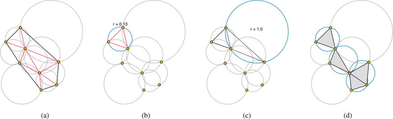
Alpha-shape example where α = 0.15: (a) convex hull (in black), Delaunay triangulation (in red), and atom centres (in yellow); (b) the k-simplex (in red) is part of the α-shape because the current circumsphere has a radius smaller than α; (c) the k-simplex (in black and dotted) is not part of the α-shape because the current circumsphere has a radius greater than α; (d) after testing each circumsphere, as seen in (b) and (c), we get the final α-shape.

By construction, the α-complex is a simplicial subcomplex of the Delaunay triangulation, where α determines the maximum admissible value of the radius of any circumsphere; the 0-complex (α = 0) reduces to the initial set of points, while ∞-complex (α = ∞) is the convex hull of the initial set of points. Therefore, the tetrahedral inscribed in circumspheres of radius greater than α are discarded from the α-complex, as illustrated in Fig. 14. By varying the value of α ∈ ℝ⁺, we obtain a filtration of subcomplexes of the Delaunay triangulation. The α-shape is defined as the union of all simplices (i.e., vertices, edges, triangles, and tetrahedra) belonging to the α-complex.

In summary, α-shape methods build upon the Delaunay triangulation of atomic centers of a given protein. The parameter α is the key idea behind a geometric carving process of generating a sub-complex of the Delaunay triangulation. The question is whether such a carving process helps anyhow in the delineation of the cavities of the molecular structure. More specifically, is there an optimal value of α ∈ ]0,∞[ to detect voids? Similarly, are there values of α that separate pockets from clefts?

8.2. APROPOS

APROPOS (Automatic PROtein Pocket Search) was introduced by Peters et al. [PFF96]. It is based on the theory of 3D α-shapes due to Edelsbrunner and Mücke [EM94]. This pocket detection method is based on the solvent-accessible surface (SAS), but, in practice, one uses a subset of atoms augmented with the radius of 1.4 Å of solvent water probe. This is important to delimit the carving process that is typical in α-shape methods.

APROPOS builds up two envelope α-shape triangulations for a given protein, each one of which corresponds to a distinct value of α. The first (outer) envelope is coarser than the second (inner) envelope; the outer envelope is constructed with α = 20 Å, while the inner envelope is generated for a value of α in the range [3.5,4.5] Å. These values of α are empirical and were obtained from experimental testing. In this manner, one ends up having an outer envelope and an inner envelope of the protein, and so cavities are in the space between these inner and outer envelopes, or α-shapes.

8.3. CAST

The main drawback of APROPOS stems from the need of tuning the value of α for both outer and inner α-shapes, in particular the one concerning the inner α-shape, which is more sensitive to the surface shape variations of the protein itself. To overcome this problem, Edelsbrunner et al. [Ede98] introduced the dual subcomplex of the union of balls featuring van der Waals atoms, which amounts to the α-shape that is entirely inside such union of balls. In essence, they proposed the convex hull as the outer envelope, and the dual subcomplex as the inner envelope of atomic coordinate centers (see Fig. 15).

Figure 15.

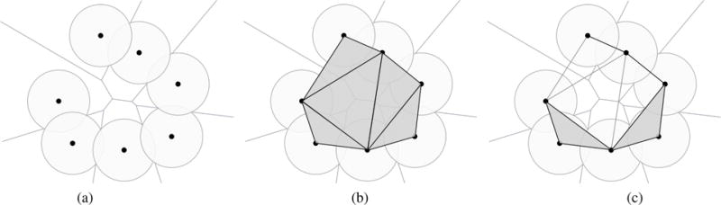
Detecting cavities through CAST: (a) Voronoi diagram of a molecule (i.e., set of spherical atoms); (b) convex hull of the atomic centres, together with Delaunay triangulation; (c) α-shape with triangles, edges, and vertices in black, where the empty triangles denote the existence of a cavity (taken and modified from [LWE98] [WPS07]).

CAST was introduced by Liang et al. [LWE98] as an implementation of the method detailed by Edelsbrunner et al. [Ede98], and consists of the following steps:

• Voronoi diagram. Firstly, one creates a Voronoi space decomposition from the atoms (atomic coordinates) of the molecule, as shown in Fig. 15(a).

• Convex hull. Secondly, one calculates the corresponding convex hull (i.e., Delaunay triangulation), as illustrated in Fig. 15(b).

• Dual subcomplex. Then, one removes the simplexes (e.g., triangles) that are not completely inside the molecule, resulting so in an α-shape of the original molecule, as depicted in Fig. 15(c).

The leading idea here is to get a triangulation with the same topological type as the original set of atoms that comprise the molecule so that we can extract the cavities in a straightforward manner. Note that we have assumed that all atoms possess the same radius (see Fig. 15). In case of using the actual van der Waals atoms, one has to use, instead, the weighted Delaunay triangulation, being the weighted Voronoi cells necessarily different.

Additionally, Edelsbrunner et al. [Ede98] introduced a discrete-flow method to decide on the existence of cavities or pockets in the complement of the dual subcomplex within the convex hull here called complement subcomplex (i.e., the subcomplex of empty or partially empty triangles). The eligibility of a cavity as part of the complement subcomplex is determined in conformity with the principle of a fluid flowing into a sink. Let us imagine the water flow field generated by filling each triangle with water, so that the water of each obtuse triangle flows to the next one until it reaches a pocket or sink represented by an acute triangle, as illustrated in Fig. 16. This means that every single pocket is formed by growing from an acute triangle.

Figure 16.

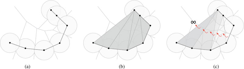
Discrete-flow method at work: (a) Voronoi space decomposition of a molecule; (b) Flow of obtuse triangles from the initial space decomposition; (c) example that shows a cavity that cannot be properly identified by the method, because the group of obtuse triangles are flowing to infinity (taken and modified from [LWE98]).

But, as Edelsbrunner et al. [Ede98] noted, some cavities cannot be identified using this discrete flow process, simply because the Delaunay triangulation can lead to the flow of obtuse triangles to the infinity, i.e., some cavities do not match acute triangles or tetrahedra. In fact, Edelsbrunner and co-authors formally defined cavities as 3D regions in the complement space of the protein that possess limited accessibility from the complement space itself. Cavities were deliberately defined in this manner to exclude shallow valleys or depressions, like the one shown in Fig. 16(b), although some shallow valleys match well-known binding sites.

Summing up, CAST does not solve the fundamental problem of the stopgaps (or delimiters) of some cavities (in particular, wide clefts/grooves), i.e., it is not always possible to know where the cavity begins and the outside space occupied by the solvent ends. Liang et al. [LWE98] identified this as a difficult problem to overcome; hence, the “can of worms” problem that they mention in their paper. In fact, in CAST, the discrete flow condition (or acute triangle condition) is not satisfied for all types of cavities; it is only valid for the types of cavities considered by Edelsbrunner et al. [Ede98] and Liang et al. [LWE98], say pockets with i mouth openings, with i = 0,1,…,n, and $n\in \text{ℕ}$.

CAST is the basis of other methods and systems, namely: CASTp web server [BNL03], SplitPocket web server [TDCL09], and RobustVoids [SDP*13], just to mention a few of them. CASTp is also based on the theory of α-shapes, and arguably can detect all pockets and voids of a given protein, as well as the surface atoms participating at each cavity. SplitPocket also uses the weighted Delaunay triangulation and the discrete flow procedure to predict each pocket of a given protein. But, unlike CAST, it utilizes not only geometric information but also physicochemical and evolutionary information (e.g., conservation index) for putative binding cavities. RobustVoids builds on the weighted Delaunay triangulation to construct a filtration of α-shapes to extract pockets and voids in a robust manner with the user assistance. The accuracy of this system comes from the fact that cavities are correctly determined independently of the small inaccuracies resulting from crystallographic measurements (X-ray crystallography) or the perturbation of atomic radii, which, as widely known, are determined empirically.

8.4. GP method

The geometric potential (GP) method is due to Xie and Bourne [XB07]. It is similar to CAST in the sense that the carving process has the effect of peeling empty triangles and tetrahedra off the convex hull (i.e., the Delaunay triangulation). However, the peeling-off of simplices is based on empirical parameters like the maximum size of 30.0 Å for a ligand binding pocket.

The steps of the GP method are the following:

• C_α atom-based structure. Firstly, one constructs the protein structure from its C_α atoms (or alpha carbon atoms), as shown in Fig. 17(a). An amino acid (or, amino acid residue, to be more precise) consists of an amino group (NH₂), a hydrogen atom (H), a carboxyl group (COOH), and a side chain (R) bound to a C_α atom [Pro14]. C_α atoms are the central atoms of amino acids that form a protein.

• Convex hull. Secondly, one constructs the convex hull (i.e., Delaunay triangulation), as illustrated in Fig. 17(b).

• First carving step. Thirdly, one proceeds to the peeling of the tetrahedra from the convex hull; this carving procedure is limited to simplexes whose edges are longer than 30.0 Å (black dashed lines), as depicted in Fig. 17(c). The resulting triangulation is bounded by the so-called environmental boundary, which functions as the outer envelope of the protein.

• Second carving step. Then, one proceeds to the further peeling of the tetrahedra circumscribed by spheres with a radius larger than 7.5 Å. This results in the inner envelope of the protein, also called protein boundary, which mostly overlaps the outer envelope. See Fig. 17(d).

• Prediction of binding cavities. Finally, it comes the time of predicting where binding cavities are, as illustrated in Fig. 17(e). For that purpose, one uses shape descriptors such as the geometric potential and residue surface direction for each C_α atom.

Figure 17.

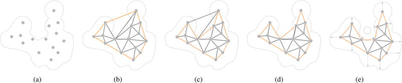
GP method [XB07]: (a) C_α atom-based structure (gray points); (b) convex hull (in orange) and Delaunay triangulation (in dark gray); (c) first carving procedure that removes simplexes whose edges are longer than 30.0 Å (black dashed line segments); the resulting environmental boundary (i.e. outer envelope of the protein) is represented by orange solid line segments; (d) second carving procedure removes k-simplexes circumscribed by spheres with radius larger than 7.5 Å (in orange); this results in the inner envelope of the protein (i.e. protein boundary); (e) geometric potential (GP) and residue surface direction are used to predict binding cavities (taken and modified from Xie and Bourne [XB07]).

The novelty of the GP method is twofold:

• The use of C_α atoms of a given protein instead of its entire set of atoms. This speeds up the algorithm because we are considering one atom per amino acid instead of its nine atoms (excluding the side chain), but it produces a very rough approximation that leads to significant geometric inaccuracies. Indeed, the GP method uses a coarser atomic structure, where each C_α atom features an amino acid.

• The use of GP parameter as a new shape descriptor capable of distinguishing cavities that bind from those that do not bind ligands.

Xie and Bourne [XB07] used the following formula

$$P=d+{\displaystyle \sum _i\frac{d_i}{D_i+1.0}}\frac{\text{cos}({\mathrm{\alpha }}_i)+1.0}{2.0}$$ (5)

to calculate the value of the geometric potential P at each C_α, where d stands for the distance of the C_α atom to the environmental boundary, d_i is the distance of its i-th neighbouring C_α atom to the environmental boundary, while D_i and α_i denote the distance and direction to its i-th neighbouring C_α atom; note that we only consider the i-th neighbouring C_α atoms belonging to the protein boundary, with the further condition that they are not obstructed by other residues within the protein boundary.

Then, it remains to calculate the geometric potential for each putative binding cavity, which is given by the average of the geometric potentials for all C_α atoms within the cavity. A cavity is considered as a ligand binding site if its geometric potential is around 50 (on the scale of 0-100); otherwise, the cavity does not qualify as ligand binding site, being its geometric potential usually close to zero.

8.5. MOLE

MOLE [PKKO07] is a follow-up of CAVER [POB*06] (see Section 7.2), both developed by Petřek and colleagues. CAVER is a grid-and-surface method, while MOLE is a Voronoi tessellation-based method, though CAVER has later evolved to incorporate Voronoi tessellations in its direct follow-ups, CAVER 2.0 [MBS08] and CAVER 3.0 [CPB*12].

As argued by Petřek et al. [PKKO07], CAVER suffers from two drawbacks: (i) the use of grid makes it very memory space and time-consuming in exploring large ramified channels; (ii) the introduction of unavoidable grid approximation errors. On the contrary, MOLE takes advantage of the Voronoi tessellation to find pathways defined by Voronoi vertices in the empty space corresponding to channels, tunnels, and pores (Figure 18). Such pathways defined by the Voronoi tessellation’s edges are found using Dijkstra’s pathfinder so that such cavities are found with greater accuracy, in less time and is fully automated when compared to CAVER. Superficial cavities like clefts/grooves are determined with the help of the convex hull that encloses the molecule.

Figure 18.

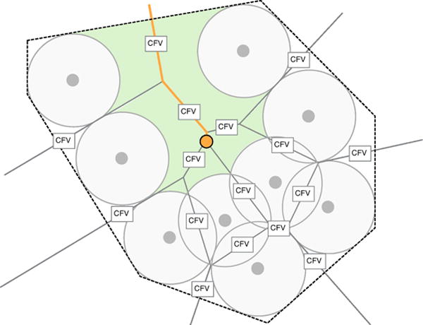
Detecting cavities using MOLE [PKKO07]: Two dimensional example of the Voronoi diagram of a molecule comprised by a set of atoms (gray spheres). The convex hull is represented as dotted black lines and each Voronoi edge is label with a cost function value (CFV). The Dijkstra’s algorithm is accomplished using each CFN from a user-given start point (orange small sphere). The path delineated by the previous algorithm (orange line) is identified as a cavity (pictures taken and modified from [PKKO07]).

See [SSVB*13] for further details about a more recent follow-up of MOLE, called MOLE 2.0, which also estimates physicochemical properties of the identified channels, such as, hydropathy, hydrophobicity, polarity, charge, and mutability.

8.6. Medek et al.’s method

This method is focused on the computation of channels, as proposed by Medek et al. [MBS07]. It is based on the Delaunay triangulation (the dual of Voronoi diagram), which has the advantage of functioning also like the envelope of the molecule, in a way similar to convex hull. Indeed, the convex hull is easily found from Delaunay triangulation. However, for performance purposes, Medek et al. do not use the exact formulation of the Delaunay triangulation of a set of points, but instead a Delaunay triangulation of a set of spheres representing atoms. See [KCK04] for further details about the Voronoi diagram of a set of spheres, also referred as the additively weighted Voronoi diagram or Euclidean Voronoi diagram of spheres.

Such a Delaunay triangulation of a set of spheres can be then interpreted as a weighted graph. Two simplifications, conservative and approximate, were introduced to give different weights to the graph. The conservative simplification sets the radii of all atoms to the biggest atom’s radius, whereas the approximate simplification assumes that all atoms have identical radii. The authors show that the ideal tunnel is obtained from the graph using a modified Dijkstra algorithm, in the sense that Dijkstra’s pathfinder is optimal and complete, it finds the lowest cost path (if it exists) along the interior of a channel. Note that Dijkstra’s pathfinder is limited by the convex hull, which significantly shortens its computation time. Both approaches provide a good trade-off between tunnel quality (without noticeable loss of accuracy) and computational time. Although the conservative simplification gives less accurate results, it is faster than its approximate counterpart due to its greater simplicity. Both simplifications show a much better ratio of speed to accuracy when compared to CAVER, although the tests only considered two molecules with little less than 2500 atoms.

8.7. Kim et al.’s method (KCC*)

One of the main limitations of α-shapes stems from the assumption that, in a set of spheres, all spheres are of the same size [KKS01a] [KKS01b] [KSK*06]. Edelsbrunner tried to solve this problem through the generalization of α-shapes to weighted α-shapes [Ede95], but, even so, they did not take into consideration the variations in size of input spheres, in the sense that the proximity among spheres is not fully described in relation to Euclidean metric [KSK*06].

With this in mind, Kim et al. [KCKC06] proposed a method based on β-shapes, which take into account distinct van der Waals (vdW) radii for atoms (Fig. 19). In this sense, beta shapes can be seen as a generalization of alpha shapes. Essentially, they proposed an algorithm that first determines the Voronoi diagram of vdW atoms of a given protein. Note that the Voronoi diagram of atoms is not the same as the ordinary Voronoi diagram for points (centers of atoms) since the Euclidean distance is measured not relative to the centers of the atoms, but relative to the surface of the atoms. After determining such extraordinary Voronoi diagram, one constructs the corresponding beta shape using a spherical probe.

Figure 19.

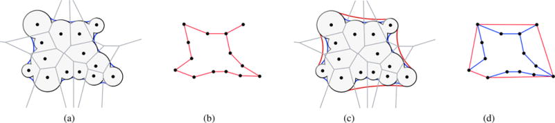
(a) van der Waals surface in black, and inner blending surface as a connected arrangement of blue and black spherical patches; (b) inner blending mesh constructed from the atomic centres and blending surface; (c) outer blending surface as a connected arrangement of red and black spherical patches; (d) outer blending mesh as the convex hull of atomic centres (taken and modified from Kim et al. [KCC*08]).

Following the same line of research, Kim et al. [KCC*08] built up a blending mesh of triangles derived from a surface generated from blending atoms, as illustrated in Fig. 19. Then, they construct the convex hull from such a blending mesh. Cavities are found in places of the convex hull that are not occupied by the blending mesh. Also, Kim et al. [KCC*08] use the Voronoi diagram of atoms, not the Voronoi diagram of atom centers, to easily calculate the molecular surface.

8.8. MolAxis

This method was developed by Yaffe et al. [YFW*08]. MolAxis relies on two geometric concepts: α-shapes and medial axis. The use of α-shapes means that the molecule is seen as a set of 3D balls featuring constant-radius atoms. In respect to the medial axis of a geometric object, it can be defined as the set of points that possess one or more closest points on the boundary of such object [Blu67]; for example, the midpoint of a straight line segment, the center of a sphere, or the axis of a cylinder. In the case of MolAxis, the geometric object at hand is the vdW surface of a molecule. Taking into account that the surface is closed in 3D, we end up having two medial axes: inner medial axis and outer medial axis. The inner medial axis can be understood as the skeleton of the molecule, while the outer medial axis is the skeleton of the complement of the molecule in 3D, i.e., the space outside the molecule.

MolAxis is focused on the computation of outer medial axis because it indicates where channels and tunnels of a molecule are. The outer medial axis is similar to Voronoi pathways of MOLE (see Section 8.5) in the complement space because MolAxis takes advantage of the inner and outer medial axes of the protein built upon the Voronoi diagram. The main novelty of MolAxis is how it approximates the outer medial axis of the complement space of the molecule to construct channels. That is, it approximates the additively weighted Voronoi diagram, as already used by Medek et al. [MBS07]. This approximation is the result of approximating each vdW atom by one or more unit balls, i.e., the weighted Voronoi diagram is approximated by the Voronoi diagram of atomic centers. But, the outer medial axis can be calculated in an exact manner using the weighted Voronoi diagram, also called Apollonius diagram [BD05].

8.9. Fpocket

Guilloux et al. [LGST09] introduced Fpocket, which primarily builds upon the Voronoi diagram of the set of centers of the atoms of a given protein (see Fig. 20). For that purpose, one computes the Voronoi tessellation of the atomic centers, what is performed using the publicly available qvoronoi’s source code at http://www.qhull.org, a well-known package that firstly calculates the convex hull of a set of points through the Quickhull algorithm. However, Fpocket does not use any triangulation.

Figure 20.

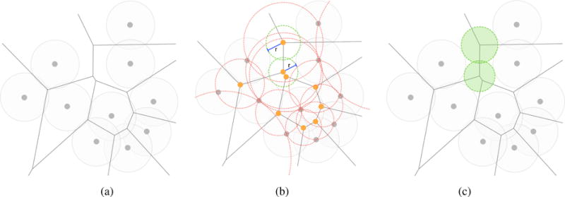
Detecting cavities through Fpocket [LGST09]: (a) Voronoi diagram of the atomic centres; (b) similar to a Voronoi ball (dotted red circles), each α-sphere (dotted green circle) is also centred at a Voronoi vertex (orange points), but it is a contact sphere that is tangential to surface atoms (solid gray circles); (c) cluster of α-spheres (solid green circles) that fill a cavity.

Instead, Fpocket uses the Voronoi tessellation and alpha spheres. Every single alpha sphere is centered at a distinct Voronoi vertex, although an alpha sphere is smaller than its homologous Voronoi ball. Its radius is given by the distance from its Voronoi vertex to the closest atom center minus the radius of such atom. Thus, alpha spheres in the complement space of a protein are tangential spheres in contact with surface atoms.

Recall that a Voronoi vertex is the center of an empty circumsphere, called Voronoi ball, through four points, which coincides with an empty circumsphere of the Delaunay triangulation; this is so because the Voronoi tessellation and Delaunay triangulation are dual structures. So, in conformity with the empty circumsphere rule of the Delaunay triangulation, an alpha sphere has always four points of contact with surface atoms, featuring thus the local curvature of the molecular surface. That is, cavities are located where we find alpha spheres; this thus requires the use of some clustering of alpha spheres to form such cavities. In other words, locating alpha spheres is equivalent to detect cavities on protein surfaces.

The main steps of the method are as follows:

• Voronoi tessellation. Firstly, one constructs the Voronoi diagram of the atomic centers, as illustrated in Fig. 20(a).

• Computation of alpha spheres. Secondly, one determines the contact alpha spheres centered at the Voronoi vertices in the complement space of the molecule. The minimum size of an alpha sphere is naturally solvent (water) probe sphere, which has 1.4 Å of radius, but bigger radii may be used. This allows us to immediately discard solvent inaccessible alpha spheres. Nevertheless, we have to define a maximum size for alpha spheres to also discard rather exposed alpha spheres. This a priori pruning of too small and big alpha spheres significantly reduces the number of false positives and false negatives for cavities. This is illustrated in Fig. 20(b).

• Clustering of alpha spheres. Thirdly, one proceeds to the clustering of alpha spheres, as shown in Fig. 20(c). The clustering procedure uses the proximity and neighborhood relationships of Voronoi vertices to aggregate their alpha spheres into separate clustered pockets within the empty complement space.

• Pocket ranking. Finally, the ranking of cavities takes place to check their ability to bind ligands. For that purpose, one uses a straightforward scoring scheme that is based on the partial least squares (PLS) regression, which is somehow related to the principal components regression. This has the effect of further reducing the number of false positives and false negatives for cavities.

8.10. CAVE

CAVE was introduced by Busa et al. [BHH*10] to solely identify voids in proteins. Its leading idea is to construct an enveloping triangulation enclosing each void. That is, it does not make usage of α-shapes, Voronoi diagram, β-shaped, or Apollonius diagram. The enveloping triangulation is a tetrahedralization whose vertices are the atomic centers, so it is a Delaunay-like triangulation in 3D.

As its authors noted, van der Waals radii of atoms are augmented by the (water) probe sphere radius. That is, the number, sizes, and shapes of cavities are strongly dependent on the probe radius. The goal is to construct a minimal closed 2-cycle (envelope) of triangles enclosing each void. Any tetrahedron’ triangle intersecting the void is not considered as being part of the minimal closed 2-cycle of a void. Let us mention that CAVE also allows for detecting voids, as well as for studying properties of each void, namely its location, boundary atoms, volume, and surface area.

8.11. VoroProt

VoroProt was proposed by Olechnovic et al. [OMV11]. It resembles MOLE and MolAxis because they are all based on the additively weighted Voronoi diagram of a set of atoms, which is also known as Apollonius diagram [EM94, EK06]. Therefore, a molecule is a set of atoms represented as vdW spheres. Then, one constructs the Apollonius diagram, which can be seen as the Voronoi diagram of the set of vdW spheres. At last, it takes place the construction of the Apollonius graph (i.e., the dual of the Apollonius diagram), which works as the delimiter of the molecule. Apollonius graph unequivocally defines the set of atoms neighboring each atom. This construction is similar to the Delaunay triangulation, with the difference that one uses spheres instead of points, and tangent spheres instead of circumspheres (circumsphere rule). As for MOLE and MolAxis, cavities in the complement space are detected using skeletal pathways (for invaginations, tunnels, and channels) in the Apollonius diagram together with the boundaries of the Apollonius graph (surface grooves and voids). Thus, there is no room for ambiguity in locating entries and exits of cavities of the molecule.

8.12. Lindow et al.’s method (LBH)

Similar to Voroprot, Lindow et. al.’s method [LBH11] also relies on the Apollonius diagram (i.e., the Voronoi diagram of spheres). It aims at identifying transport pathways in molecules. Such pathways are determined using depth-first search in the graph built from the edges and nodes of the Apollonius diagram.

Unlike Voroprot, Lindow et al. did not use the Apollonius graph as a delimiter of the molecule. Instead, they used omnidirectional casting of rays from every single Apollonius vertex to determine whether it lies in a cavity of not; more specifically, if more than 50% of rays hit the molecular surface, one conclude that the vertex belongs to a cavity. This threshold of 0.5 is a value that leads to approximately discard the vertices outside the convex hull of the molecule. Therefore, there is no ambiguity in identifying cavity entries and exits.

8.13. BetaVoid

BetaVoid was introduced by Kim et al. [KCL*14] to identify voids exclusively, i.e., the method was not designed to identify cavities in general. It is a freeware solution for molecular void recognition and accurate computation of void volume, area, and topology. It relies on a geometric formalization of molecular voids allied with an analytic approach that uses the Voronoi diagram of spherical atoms and the β-complex. The proposed algorithms identify both van der Waals and Lee-Richards solvent-accessible voids, along with the residues that belong to each void atom. Also, BetaVoid allows users to vary atom radii from the default values of the Bondi radii. One of its main contributions is a general and unified geometric framework that allows us to analyze molecular voids in an efficient and mathematically correct manner.

8.14. CCCPP

More recently, Benkaidali et al. [BAM*14] introduced an alpha-shape variant, called CCCPP, which supposedly takes advantage of the size and the shape of the ligand. This method essentially finds the empty space where channels, pockets, and cavities are in the complement of the alpha shape of the protein to its convex hull. That is, the convex hull works here as the outer envelope of the protein.

Therefore, the convex hull works as the ceiling for each concavity of the protein. As their authors argued, the focus of the method is on the shape of the channels (i.e., empty space inside the convex hull), not the shape of the protein. To find those channels, one uses a door-in-door-out principle for empty (or partially) tetrahedra. This principle is similar to the discrete flow principle, with the difference that now the convex hull is functioning as the outer boundary for all channels.

Channels are found as follows. Starting from the Delaunay triangulation, one constructs a graph for empty (or partially empty) tetrahedra inside the convex hull. This is a graph whose nodes represent empty (or partially empty) tetrahedra, and edges represent triangles bounding those tetrahedra, much like we do in the construction of the Voronoi diagram from the Delaunay triangulation, with the difference that we are not imposing any geometric constraints to such graph, here called facial graph. A channel is a connected subgraph of the facial graph.

Note that Benkaidali et al. argue that the spherical model for ligands, usually given by a probe sphere featuring a water molecule is often not adequate for the detection of channels, so they ended up by applying the cylindrical model instead. The adoption of the cylindrical model is seen by the authors as a step forward in the conventional alpha-shape approaches.

8.15. Tessellation-based methods: discussion

Looking at Table 6, we come across that tessellation-based methods, we observe the following:

• Molecular Surfaces. These methods do not use any molecular surface. To identify molecular cavities, they only use vdW atoms or their centers; at most, we can say that they indirectly use the vdW surface. More specifically, α-shape and Voronoi-based methods use atomic centers and, implicitly constant-radius spheres to represent atoms, while β-shape methods and Apollonius-based methods take advantage of varying-radius spheres to represent those atoms.

• Limitations. As shown in Table 6, tessellation-based methods do not suffer from significant limitations indeed. In a way, these limitations are all related to accuracy in identifying not only the correct location of each binding cavity of a given protein, but also its number of surface atoms and its boundary —and, subsequently, its area and volume— in the complement space. In respect to α-shape methods, they are focused on the occupied space by a protein so that any tiny empty space less than a water molecule inside a tetrahedron originates a false positive. Also, two buried chambers interconnected via a small channel with a radius less than the water molecule is reported as a single cavity, when it consists of two distinct cavities or a cavity with two sub-cavities. This shows that alpha shapes are sensitive to false negatives. In fact, α-shape methods tend to fail to detect wide surface pockets and shallow valleys. On the other hand, β-shape methods produce more accurate results than α-based methods because they are based on vdW atom-featuring spheres instead of atomic centers.

  On the contrary, Voronoi-based methods put their focus on the empty complement space, filling it with contact spheres, called alpha spheres, centered at Voronoi vertices. By using the least radius of 1.4 Å for alpha spheres, one guarantees the number of false positives and false negatives is reduced to a minimum. The cavities are where there is a higher density of contact spheres. Furthermore, they provide a skeleton per channel in a way similar to medial axis. Finally, Apollonius-based methods produce more accurate results than Voronoi-based methods, because they are based on vdW atom-featuring spheres instead of atomic centers. For example, the skeletal pathways of channels approximate the medial axis of the complement space.

• Cavities. With the exception of a few cavity detection methods, we can say that tessellation-based methods are accurate in identifying cavities of proteins. In general, Voronoi- and Apollonius-based methods are adequate to identify any cavity, in particular channels; surface pockets are also easily identified because of the use of the convex hull, Delaunay triangulation, or Apollonius graph, which work as delimiters of the protein.

Table 6.

Tessellation-based methods.

Methods	Reference	Tessellation	Molecular Surfaces		Limitations		Cavities
			SA/vdW	CH	EAT	MOA	Pockets			Channels	Voids
							Clefts / Grooves	Invaginations	Tunnels
APROPOS	[PFF96]	α	●		●	●	●	●	●	●	●
CAST	[LWE98]	α	●	●		●	●	●	●	●	●
GP	[XB07]	α	●	●	●	●	●	●	●	●	●
MOLE	[PKKO07]	AD	●	●			●	●	●	●	●
Medek et. al.	[MBS07]	DT	●	●					●	●
KCC*	[KCC*08]	β	●	●		●	●
MolAxis	[YFW*08]	AD, MA	●				●	●	●	●	●
Fpocket	[LGST09]	α, Voronoi	●				●	●
CAVE	[BHH*10]	ET	●			●					●
VoroProt	[OMV11]	AD	●				●	●	●	●	●
LBH	[LBH11]	AD	●	●			●	●	●	●	●
BetaVoid	[KCL*14]	α	●								●
CCCPP	[BAM*14]	α	●	●			●	●	●	●	●

Abbreviations: AD: Apollonius diagram [EK06]; DT: Delaunay triangulation; MA: medial axis [Blu67]; ET: enveloping triangulation [BHH*09]. SA/vdW: set of atoms / van der Waals surface; CH: convex hull. EAT: empirical alpha tuning; MOA: mouth-opening ambiguity.

As far as we know, there is not any tessellation-based method in the literature to identify cavities into sub-cavities. Nevertheless, it is straightforward to accomplish that with Voronoi- and Apollonius-based methods because they produce skeletal pathways and their branches.

9. Consensus Methods

To the best of our knowledge, Metapocket is the only consensus method found in the literature, which was proposed by Huang [Hua09]. Consensus methods are approaches that combine the results produced by two or more cavity detection techniques. More specifically, this method combines the predictions of four methods to improve the success rate in predicting the location of binding cavities; three of these methods are purely geometric (LIGSITE^cs, PASS and SURFNET), while the fourth is an energy-based method (Q-SiteFinder [LJ05]).

Since these four methods have different ranking scoring functions, it is hard to compare and evaluate the predictions directly. Therefore, a z-score is calculated separately for each cavity using different methods, to make the ranking scores comparable. Probes within a given distance threshold are grouped together as a cluster, and each cluster is ranked by a scoring function consisting of the sum of the z-scores of the cavities in that cluster. For the dataset of proteins referred by Huang [Hua09], MetaPocket improved the success rate up to 90% over individual methods.

Later, Zhang et al. [ZLL*11] continued this work by adding more four methods (GHECOM, ConCavity, POCASA, and Fpocket) to further improve the prediction success rate. This resulted in the development of MetaPocket 2.0, a consensus method which combines the predicted cavity sites of a total of eight methods.

10. GPU-Based Methods

In the last decade, we have noted an increasing use of GPU computing in molecular modeling, rendering, and visualization [KBE09, SSE*10, DBG10, LBH11, KKC*11, CVT*11, PTRV12, TPS12, PRV13, DG13, PTRV13, LLNW14, DCD*14, DG15, HGVV16]. However cavity detection methods taking advantage of GPU processing power are not so commonly found in the literature; the exception lies in the methods we describe below.

10.1. Parulek et al.’s method

After introducing an implicitly-defined formulation for SES (solvent-excluded surface) [PTRV12], Parulek et al. [PTRV13] proposed a cavity detection algorithm solely for molecular visualization purposes, i.e., they were not concerned about benchmarking the accuracy of their algorithm against a ground-truth of already known binding cavities. Arguably, most computations were performed on GPU using CUDA and GLSL, but no details about the implementation of their method were published.

Therefore, this is a surface-based method, which has the particularity of using a random sampling of the domain, much like in McVol [TU10] (see Section 5.4). More specifically, they generate point samples inside balls centered at atomic centers, but with a radius that is twice the vdW radius of each atom. The samples inside SES are dropped straight away. The remaining samples outside SES are used to determine the cavities on SES.

Parulek et al. take advantage of an implicit formulation of SES to determine the direction of the gradient at each point sample outside SES. Similar to grid-based methods with scanning directions, this gradient vector and its symmetric vector determine the existence of a cavity if they hit two opposite boundary walls of SES. As the last step, they use mutual visibility test between pairs of points satisfying the scanning direction condition between walls of SES with the goal of clustering the sampled points into distinct cavities. However, as the authors mentioned in their paper, their method may not identify all and especially shallow cavities [PRV13].

10.2. Krone et al.’s method

Similar to Parulek et al.’s method, Krone et al. [KRS*13] used an implicit formulation for molecular surfaces, not only for representing and modeling molecular surfaces but also to help in extracting the molecular cavities for visualization purposes. More specifically, they use a Gaussian surface that better adjusts to SES, in conformity with the parameter set in [GP95] and [Ric77]. This work is a follow-up of their previous work detailed in [KFR*11], which arguably was the first method to extract cavities in real-time extraction. Cavities are detected using an ambient occlusion-based visibility criterion due to Borland [Bor11], who used an ambient occlusion-based approach to get an adequate visualization of the internal structure of proteins. Once again, this method focuses on molecular rendering and visualization of cavities, and not on the accuracy of the method in detecting and locating cavities, even with respect to benchmark results.

Thus, the leading idea of the method was to obtain a surface segmentation with noticeable cavities. For that purpose, the molecular surface is triangulated beforehand using the marching tetrahedra algorithm due to Doi and Koide [DK91]. The resulting triangles are then tagged as either shadowed or unshadowed, what depends on their computed ambient occlusion (AO) factors in relation to an user-defined threshold. It is clear that shadowed triangles are those that belong to eventual cavities so that they are clustered into cavities using the principle of connectedness, i.e., two adjacent shadowed triangles in the molecular surface belong to the same cavity. This clustering-based segmentation is based on the labeling technique due to Hawick et al. [HLP10], which was specially designed for GPU computing. However, because it mostly aims at molecular visualization, its authors did not embark in any benchmarking with other cavity detection method regarding accuracy (e.g., the number of cavities and their locations).

10.3. PLB-SAVE

To the best of our knowledge, the first cavity detection method to run entirely on GPU (via CUDA) is due to Lo et al. [LWP*13], and is called PLB-SAVE. Furthermore, it uses the LigASite dataset of binding sites for benchmarking comparisons [DLW08].

The leading idea of this method is to take advantage of the Connolly function for segmentation of the molecular surface into cavities and its complement. While using the Connolly function to divide the molecular surface into convex, concave, and saddle patches is not a novelty [CCL03], their segmentation produces numerous fine patches to be useful in cavity detection. One ideally requires a coarser surface segmentation, and especially with larger binding cavities. Natarajan et al. [NWB*06] introduced a Morse theory-based segmentation of molecular surfaces to solve this problem. Instead of using the Connolly function, Natarajan et al. used the Mitchell-Kerr-Eyck function [MKE01] as a way to merge neighbor segments into larger segments by simplifying the atomic density function.

PLB-SAVE essentially is a grid-based method applied to the set of atoms of a given molecule. This method maps each atom over their occupied voxels in the 3D space. This way, one can identify the protein surface, from which one calculates the solid angles associated with each atom. In practice, PLB-SAVE thus uses a discrete version of the Connolly function. Instead of measuring the solid angle Ω associated to each surface point, one measures the solid angle of each surface voxel, which is given by the following expression:

$$\mathrm{\Omega }=\frac{n}{N}\cdot 4\mathrm{\pi }$$ (6)

where N is the whole number of voxels occupied by a probe sphere of 6 Å centred at each surface voxel, and n denotes the number of those voxels overlapping the protein. This means that Ω ∈ [0,4π]; if Ω ∈ [0,2π[, the corresponding surface voxel lies in a convex region of the surface; if Ω ∈ ]2π,4π], the corresponding surface voxel is located in a concave region of the surface; if Ω ≈ 2π, the corresponding voxel belongs to an approximately flat region of the surface.

Next, one proceeds to the clustering of connected surface voxels around those with similar, highest solid angles, i.e., only the concave regions concerning cavities are taken into account. Note, that the Connolly function is translation- and rotation-invariant because it is defined over the molecular surface. However, clustering voxels with similar solid angle levels can often lead to misleading results (i.e. unreliable cavity locations). This is so because a binding cavity may include concave and approximately flat regions, as a result of the fine-grain segmentation that results from the Connolly function. To overcome this problem of significant variations in the solid angle of a cluster of voxels, Lo et al. introduced the concept of average depth for a cavity [LWP*13].

10.4. CAVE-CL

CAVE-CL is an OpenCL implementation of the CAVE method that is authored by Buša et al. [BHH*09, BHH*10, BHHW15]. This method was designed to detect voids solely, also called internal cavities. CAVE-CL operates on a set of balls featuring the atoms of a molecule, but the size of each atom is increased with the radius of the probe sphere, as is usual for the solvent-accessible surface (SAS).

The atom centers are vertices of the so-called envelope triangulation (ET), which can be seen as a subcomplex (or subset) of the nerve of an alpha shape triangulation. After building up this envelope triangulation, we are ready to detect where the voids of the protein are. Each void is commonly encountered inside a closed polyhedron that makes part of the envelope triangulation.

10.5. Kim et al.’s method (KLKK)

KLKK is a hybrid method due to Kim et. al. [KLKK16], which is capable of detecting voids, chambers, tunnels, and channels. It operates simultaneously on two GPU data structures (via CUDA): a sphere tree and a grid of voxels. The sphere tree is a novel representation of a given protein (i.e., the set of atoms). In fact, one generates a sphere tree for each peptide chain of a given protein; a sphere tree is held in GPU memory as a 1-dimensional array. This new representation of a protein allows us to accelerate the proximity search queries on GPUs.

After forming the sphere tree, one constructs an approximate convex hull that encloses the protein with the help of such proximity queries on the GPU. The voxels inside an approximate convex hull of the molecule are then classified as follows: occupied, empty, and empty-boundary. The voxels occupied by a given protein denote the absence of cavities; the empty voxels —in particular those containing Voronoi edges— identify the location of cavities on or inside the protein; the empty-boundary voxels are those that identify exit/entrance doors for channels and tunnels. Furthermore, this method uses the Dijkstra algorithm to determine the shortest path from a chamber to an exit mouth of a tunnel or channel. Note that KLKK takes advantage of an approximate convex hull of the molecule to distinguish the empty voxels of cavities inside the convex hull from those empty voxels outside the convex hull.

10.6. CriticalFinder

CriticalFinder is a grid-and-surface method proposed by Dias et al. [DNJG17], whose program entirely runs on GPU via CUDA. This method builds upon the theory of critical points (also known as Morse theory), and relies on the assumption that each cavity can be identified by a cluster of approximate critical points of the same sort. These approximate critical points are corners of voxels intersecting the Gaussian surface that encloses the protein. The result is a meaningful segmentation of the protein surface into cavities and saliences.

CriticalFinder calculates the approximate critical points of the Gaussian scalar field (or function) that describes the molecular surface through the eigenvalues of its Hessian matrix, i.e., it takes advantage of curvature analysis. Other research works have already used curvature information (e.g., Natarajan et al. [NWB*06]) to segment molecular surfaces. However, there is no evidence that the resulting segmentation is a meaningful segmentation in terms of cavities, because no comparison was carried out relative to any ground-truth dataset of known binding sites (e.g., LigASite at http://ligasite.org/).

10.7. GPU-based Methods: Discussion

Given the new advances in parallel computing (e.g. GPU-based applications) in last decade, we decided to define a category specifically dedicated to GPU-based methods, although they are clearly framed in geometric categories, as indicated in Table 7. Let us then discuss the characteristics of these methods:

• Molecular Surfaces. Despite the fact that these six methods belong to three different geometric categories, they all rely on the set of atoms (SA) or van der Waals surface of the protein. Nevertheless, Parulek et al. [PTRV13], Krone et al. [KRS*13], and KLKK [KLKK16] also take advantage of surface formulations as the solvent-excluded-surface (SES), Gaussian surface (GS), and convex hull (CH), respectively, to represent the molecular surface somehow.

• Limitations. Taking into consideration that every single GPU-based method belongs to some geometric category of methods, each one of them suffers from the limitations inherent to its category. For example, PLB-SAVE and KLKK are grid-based methods, so they are sensitive to grid spacing (GSS), but because KLKK uses the convex hull as the outer envelope of the molecule, it does suffer from mouth-opening ambiguity (MOA). PLB-SAVE is partially ambiguous because of the strict threshold used to classify the convex and concave surface regions through a discrete variant of the Connolly function; as a consequence, it tends to miss shallow grooves. On the other hand, Parulek et al. and Krone et al. are surface-based methods, but Parulek et al.’s method may miss identifying shallow grooves on the molecular surface because the random domain sampling may not sample such cavities in a proper way.

• Cavities. As expected, these methods are capable of correctly identifying most cavities of proteins. Nevertheless, as explained above, both Parulek et al.’s and PLB-SAVE may miss shallow grooves because of their criteria to identify cavities. As an exception, CAVE-CL, a parallel variant of CAVE (see Section 8.10), was designed to detect voids solely.

Table 7.

GPU-based methods.

Methods	Reference	Molecular Surfaces				GPU Computing	Limitations		Cavities					Category
		SA/vdW	SES	GS	CH		GSS	MOA	Pockets			Channels	Voids
									Clefts / Grooves	Invaginations	Tunnels
Parulek et al.	[PTRV13]	●	●			CUDA/GLSL		●		●	●	●	●	Surface-based
Krone et al.	[KRS*13]	●		●		CUDA			●	●	●	●	●	Surface-based
PLB-SAVE	[LWP*13]	●				CUDA	●	●		●	●	●	●	Grid-based
CAVE-CL	[BHHW15]	●				OpenCL							●	Tessellation-based
KLKK	[KLKK16]	●			●	CUDA	●		●	●	●	●	●	Grid-based; Voronoi
CriticalFinder	[DNJG17]	●		●		CUDA		●	●	●	●	●	●	Grid-and-surface-based

Abbreviations: SA/vdW: set of atoms / van der Waals surface; SES: solvent-excluded-surface; GS: gaussian surface; CH convex hull. GSS: grid-spacing sensitivity; MOA: mouth-opening ambiguity.

As seen from Table 7, the grid-based methods are still in their infancy, so a long way has to be traced in relation to n-part cavity detection (i.e., sub-cavities). Furthermore, there is not yet a benchmarking tool to compare different methods regarding performance and accuracy.

Finally, in terms of performance, most GPU implementations of the methods described above were compared with their CPU counterparts [KRS*13, LWP*13, BHHW15]. In contrast, Kim et al. [KLKK16] only benchmarked the GPU implementation of their algorithm using an increasing number of GPUs, while Dias et al. [DNJG17] adopted both strategies, CPU-GPU and multiple GPU-GPU. As expected, the use of a GPU setup speeds up the execution of the programs relative to CPU setup, and the performance boost is also noticeable when the number of GPUs increases, particularly for proteins with a large number of atoms (approx. 100,000 atoms or more).

11. Time-Varying Methods

The cavity detection methods discussed above apply to a single protein conformation at a given time, i.e., to a static structure. However, protein molecules, along with their cavities, are dynamically changing their conformation and shape over time. In fact, a major problem with static cavity detection methods is that they miss cavities that become only accessible in dynamic molecular conformations that are different to the crystal conformation [EH07]. However, in the last decade, a few works have addressed tracking the geometric evolution of molecular cavities throughout the course of molecular dynamics (MD) trajectories, as the protein molecule switches between a sequence of stable conformation states. In a more general setting, the reader is referred to Al-Bluwin et al. [ABSC12] for more details. A summary of these methods can be found in Table 8.

Table 8.

Time-Varying methods.

Methods	Reference	Core Method	Category	Dynamic Trajectories	Cavities
					Pockets			Channels	Voids
					Clefts Grooves	Invaginations	Tunnels
EPOSBP	[EH07]	PASS	Sphere-based	MD	●	●	●	●	●
TexMol	[BGG*10]	TexMol	Surface-based	NMA	●	●	●	●	●
dxTuber	[RK11]	dxTuber	Grid-and-sphere-based	MD	●		●		●
MDpocket	[SBCLB11]	Fpocket	Voronoi, Grid-based	MD	●	●
PocketAnalyzerPCA	[CPG*11]	LIGSITE	Grid-based	MD, PCA	●	●	●	●	●
Provar	[AMA*12]	PASS, Fpocket, LIGSITE	Sphere, Grid-based, Voronoi	MD, ED, NMA, CBM	●	●	●	●	●
PPIAnalyzer	[MPK*12]	LIGSITE	Grid-based	MD, FRODA	●	●	●	●
CAVER3.0	[CPB*12]	CAVER 2.0	Voronoi	MD	●	●	●	●	●
TRAPP	[KRH*13]	TRAPP	Grid-based	MD, PCA	●
LBBH	[LBBH13]	LBH	Tessellation-based	MD	●	●	●	●	●
trj_cavity	[PEG*14]	trj_cavity	Grid-based	MD	●	●	●	●	●
Epock	[LCC*15]	POVME	Grid-based	MD				●	●
Desdouits et al.	[DNB15]	GHECOM	Grid-and-sphere-based	MD, PCA	●	●	●	●	●

Abbreviations: NMA: normal mode analysis; MD: molecular dynamics; PCA: principal component analysis; ED: essential dynamics; CBM: constraint-based methods; FRODA constrained geometric.

11.1. EPOS^BP

Seemingly, EPOS^BP was the former method to detect and track transient protein cavities across a sequence of MD snapshots (or time steps) [EH07]. EPOS^BP aims at protein-protein interactions. It is based on PASS (see Section 3.4), which is a sphere-based method. Essentially, for a significant number of MD snapshots, the PASS method is used to identify the protein cavities in each snapshot. Each cavity is given an ID to track it during MD trajectories. Surprisingly, Eyrisch and Helms [EH07] noted that all cavities change over the time window of 10 ns, i.e., they vanished and reappeared several times over time. Note that to simulate a narrow lapse of 10 ns of biological time may require computing resources of CPU-weeks.

Another surprising result was the fact that transient protein cavities are one order of magnitude more than the number of cavities identified for the crystal structures of the apo proteins. This shows that time-varying cavity detection methods are particularly useful in elucidating unknown binding sites, i.e., the protein crystal structure lacks information about those missed binding cavities.

11.2. TexMol

TexMol (Texture Molecular Viewer) is a molecular visualization client software that provides a user interface to a set of software packages, including the one concerning detection and tracking methods for pockets and tunnels [BDST04].

Unlike EPOS^BP, which is based on MD trajectories, TexMol uses normal mode analysis (NMA) for the computation of small and large time-scale molecular trajectories [BGG*10]. Note that MD runs on the scale of nanoseconds to microseconds, and needs Brownian motion trajectory filtering to tune simulation results. On the other hand, NMA yields longer range molecular trajectories (on the scale of milliseconds to seconds), and trajectory filtering is obtained by selecting a subset k of the eigenmodes of the eigenmode expansion (EME).

Based on the techniques described in Section 6, Bajaj and co-authors [SB06, BGG09] take advantage of time-varying contour trees to track birth, growth, and dissolution of cavities (topology), as well as to compute stable manifolds on these NMA molecular trajectories to track the change of the mouths of cavities (geometry).

11.3. dxTuber

In the line of the time-varying methods, which usually detect cavities for an ensemble of conformations, Raunest and Kandt [RK11] developed a mixed grid-and-sphere based technique, called dxTuber, which does not neglect alternate protein forms and relies on cavity dynamics. Their technique is capable of detecting all three main types of cavities (voids, channels, and pockets) by making use of protein flexibility and solvent residence probabilities, which are derived from molecular dynamics simulations, using solvent molecules to probe for cavities. Therefore, dxTuber allows studying cavities from a molecular dynamics perspective.

Solvent and protein trajectories computed via molecular dynamics (MD) simulations are converted to a voxel representation of mass-weighed spatial density maps using VMD [HDS96], which outputs protein-internal and protein-external solvent regions. dxTuber then separates both voxel regions and classifies a cavity as a contiguous voxel set of protein-internal regions of high solvent residence probability.

For each type of cavity, a different search algorithm was implemented. Also, dxTuber was compared with SURFNET, CAVER, and PyMol to evaluate its computational performance. Only six proteins that contain the most representative protein cavities (voids, channels, and pockets) were tested. Since dxTuber relies on molecular dynamics to probe protein cavities, this technique requires a large amount of computational power to perform cavity analysis. Therefore, simulation length, molecular size, and voxel resolution directly determine dxTuber’s performance.

11.4. MDpocket

MDpocket relies on Fpocket (see Section 8.9) [SBCLB11]. Recall that Fpocket builds upon the Voronoi tessellation to detect protein cavities. It returns such cavities as clusters of α-spheres that are tangential to surface atoms of a given protein.

Tracking of transient cavities is performed using an axis-aligned grid of nodes equally spaced, with the each voxel having the size (volume) of 1.0 ų. Firstly, Fpocket is run in each snapshot, i.e., Fpocket is executed as many times as the number n of pre-defined snapshots. Secondly, for each snapshot l, each α-sphere is assigned to the closest grid node (i, j, k), being then the number α_l of counted α-spheres normalized by the number of snapshots as follows:

$${\mathrm{\rho }}_{(i,j,k)}=\frac{1}{n}{\displaystyle \sum _{l=1}^n{\mathrm{\alpha }}_l}$$ (7)

where n stands for the number of snapshots. It is clear that this originates a cavity density map ρ within the grid. This cavity density map indicates how many α-spheres are packed within cavities of the complement space.

Thirdly, for each snapshot l, each grid node (i, j,k) is given a binary occupancy parameter δ_l, i.e., δ_l = 1 if the node has been assigned at least an α-sphere; otherwise, δ_l = 0. It follows a cavity frequency map Φ over the grid, which is generated through the normalization of the binary occupancy parameter δ_l associated to each node (i, j,k) across the sequence of snapshots as follows:

$${\mathrm{\Phi }}_{(i,j,k)}=\frac{1}{n}{\displaystyle \sum _{l=1}^n{\mathrm{\delta }}_l}$$ (8)

This means that the grid node (i, j,k) is persistently accessible to the solvent if Φ_(i,j,k) = 1, blocked if Φ_(i,j,k) = 0, and transiently accessible if 0 < Φ_(i,j,k) < 1. Summing up, encoding cavities in a grid over time allows us to track cavities during MD trajectories. Thus, MDpocket renders a more generic and less error-prone identifying and tracking technique for cavities than EPOS^BP, provided that ID labeling is unnecessary.

11.5. PocketAnalyzer^PCA

PocketAnalyzer^PCA is another method to detect and track dynamic cavities along MD trajectories [CPG*11]. It was developed aiming at the characterization of protein-ligand interactions. It implements a variant of the grid-based cavity detection algorithm LIGSITE (see Section 4.3) to identify cavities —as connected aggregates of grid nodes— in each snapshot (or time step), as well as principal component analysis (PCA) to track the shape evolution of cavities.

More specifically, this method applies PCA directly on the grid nodes of each cavity, with the purpose of unveiling the dominant deformation of the cavity over time. Note that the PCA might also be applied to the atomic centers, in which case we would have to guarantee that PCA would be applied to all the atoms bordering the cavity; otherwise, some cavities may not be identified. As an example, only using C_α atoms in the computation of MD trajectories makes some cavities undetected.

This method involves two major steps: PCA and clustering. The PCA step provides the following: (i) principal component (PC) eigenvectors, which unveil the dominant deformation modes of the cavity, and (ii) PC projections (called “scores”) that characterize the cavity conformational distribution (CCD). In the second step, clustering of the CCD results of a given protein that deforms over time allows us to reduce the entire set of its structures to a small subset that holds noticeably different binding pocket conformations.

11.6. Provar

Provar (Probability of variation) was developed by Ashford et al. [AMA*12]. As other cavity tracking methods, the leading idea of Provar is gaining insight into binding cavities through the inspection of time-varying conformations of any protein. As suggested above, the argument is that the cavity prediction based on a single static structure may fail to detect putative binding sites, in particular, transient cavities that change in their shape and size over time; persistent cavities are less prone to be left out.

Provar admits, as input, sequences of conformational variants (or conformations) of a single protein produced from a number of sources, namely: molecular dynamics (MD), essential dynamics (ED), normal mode analysis (NMA), or constraint-based methods (CBM) (e.g., CONCOORD and tCONCOORD), solution-NMR conformational ensembles, multiple protein structures solved in distinct crystal forms, or with distinct ligands or experimental conditions. The detection of cavities for each conformation of the same protein can be performed using PASS, LIGSITE or Fpocket. Provar automatically identifies and scores cavity-lining atoms and residues, i.e., those atoms and residues bounding each cavity, after which it undertakes the probabilistic analysis of changes of cavities on protein surface in terms of shape and size.

11.7. PPIAnalyzer

PPIAnalyzer is due to Metz et al. [MPK*12]. It is targeted at protein-protein interactions (PPIs). Metz and co-authors noted two challenges to bear in mind in dealing with PPIs. First, in contrast to protein-ligand bindings, protein-protein interfaces —enabling the interaction between proteins— are rather flat, i.e., they lack a noticeable binding cavity. Second, taking into account the commonly large size of protein-protein interfaces —which may vary in the range 1200 to 4660 Ų approximately—, protein-protein binding tends to be broader in terms of occupied area of the interface.

In fact, as noted by Metz et al. [MPK*12], the experimental evidence suggests that residues participating in protein-protein interactions tend to be spatially clustered in protein-protein interfaces, resulting in the so-called “hot spot” regions. Furthermore, it was also observed an opening of transient cavities in protein-protein interfaces. Therefore, one concludes that to determine protein-protein interfaces, one has to look for hot spots and transient cavities.

This method works as follows. First, one uses and compares molecular dynamics (MD) and constrained geometric (FRODA) simulations to generate structural ensembles. Second, PPIAnalyzer proceeds to the analysis of structural properties of protein-protein interfaces in such ensembles, with the goal of identifying transient cavities exclusively using geometric criteria. Third, one identifies hot spots and ranks protein-protein interface modulators (PPIMs) by applying the molecular mechanics Poisson-Boltzmann (generalized Born) surface area (MM-PB(GB)SA) approach.

11.8. CAVER 3.0

CAVER 3.0 was proposed by Chovancova et al. [CPB*12] as a time-varying follow-up of the previous CAVER (see Section 7.2) method to predict tunnels and channels, which play an important role as transport pathways of water solvent, ions and small molecules in many proteins. While CAVER applies to static macromolecular structures, CAVER 3.0 was designed to cope with transient tunnels and channels over time. Moreover, CAVER 3.0 puts forward new algorithms capable of identifying and clustering such transport pathways. CAVER 3.0 was also incorporated as part of the CAVER Analyst 1.0 graphic tool [KSS*14].

The method of CAVER 3.0 consists of three steps: (i) identification of pathways for each MD simulation’s snapshot; (ii) clustering of such pathways across all snapshots; and (iii) ranking of pathway clusters. Note that the steps concerning the identification and clustering of pathways are independent of each other, so that their calculation within distinct snapshots can be performed in parallel.

The identification of pathways (first step) within each snapshot starts with the construction of a pseudo-Voronoi diagram of a given protein. Let r the vdW radius of the smallest atom of the protein. Every single atom with a radius greater than r is approximated by a user-specified number of balls of radius r, i.e., each large atom is approximated by a set of smallest pseudo-atoms. The idea here is to approximate the weighted Voronoi diagram (also known as Apollonius diagram) of a set of atoms through the ordinary Voronoi diagram of an augmented set of atomic centers. Then, as usual, pathways are identified as graph paths made up of Voronoi vertices and edges.

After detecting pathways within each snapshot, these are clustered (second step) regarding their geometric similarities (e.g., geometric distance). To identify the same cavity in disparate snapshots, the authors have proposed a modification of the average-link hierarchical clustering algorithm [LPFL08] by computing on-the-fly the distance between pathways.

Each cluster is then ranked by priority p = k/n, where k is the sum of throughputs of all pathways in such a cluster, and n is the total number of snapshots of the MD simulation. This means that both the number of pathways and their throughputs in a cluster contribute to its ranking. It is clear that, if the cluster contains two or pathways in the same snapshot, only the highest-throughput pathway is taken into account.

11.9. Lindow et al.’s method (LBBH)

This method was proposed by Lindow et al. [LBBH13], and it is here also named LBBH method after its authors. It extends the LBH method [LBH11] designed for a single conformation of a molecule and its cavities to dynamic cavities in molecular dynamics trajectories. This method consists of two steps: pre-processing step and interactive step.

The pre-processing step consists in computing the Apollonius diagram (i.e., Voronoi diagram of wdW spheres), which represents the skeletal structure of cavities, for each molecular simulation’s snapshot. In other words, this step aims at computing the static molecular paths for each snapshot in a separate manner, as in a authors’ previous work [LBH11].

In mathematical terms, a static molecular path is nothing more than a subset of the skeleton of the distance function determined by the vdW spheres; specifically, it consists of maxima and index-2 saddles and maxima of such a distance function, together with their interconnecting separatrices.

The interactive step allows the user to identify, choose and visualize the dynamic cavities and their changes over time, i.e., users observe how dynamic molecular paths (cavities) evolve over time.

11.10. TRAPP

Kokh et al. [KRH*13] introduced TRAPP (TRAnsient Pockets in Proteins). TRAPP works on ensembles of protein conformations obtained from simulations or from experimental structures, from which it is capable of identifying the stable and transient regions of cavities in an automated manner.

TRAPP uses a grid-based method for cavity detection that determines the shape and physical properties of every single binding site. The detection of transient cavity regions is performed using two distinct techniques. The first takes advantage of principal component analysis (PCA) to correlate cavity variations, muck like in PocketAnalyzer^PCA. The second calculates the averaged deviation of the cavity shape in a molecular trajectory (i.e., across an ensemble of structures or conformations of a given protein) relative to a reference (crystal) structure; such a deviation was named the averaged relative deviation from a reference structure (ARDR).

This method distinguishes itself from others in that it only considers binding sites for which there are already known ligands. To validate the ability of TRAPP in detecting stable and transient cavities, their authors used a set of holo-proteins and already known protein motion trajectories, more specifically, trajectories generated by standard MD simulation over 10 ns, which are available from the MoDEL database [MDH*10].

11.11. trj_cavity

trj_cavity was developed by Paramo et al. [PEG*14] within the GROMACS (www.gromacs.org) framework for quickly identifying and characterizing cavities detected along MD trajectories. The method is based on a new grid-based approach to detect cavities on each frame (or snapshot) by efficiently searching neighbor voxels; in fact, its time complexity is linear with respect to the number of voxels. More specifically, trj_cavity searches for each voxel belonging to a cavity along each of six directions defined by the positive and negative x, y, and z axes. The method can detect cavities along the trajectory by assuming that the next frame has the same cavity on the current frame, and they overlap somehow partially in space.

The performance of trj_cavity is heavily dependent on some parameters, which include the voxel size and the number of cavities that the user aims to detect, e.g., cavities with a predefined value volume. Furthermore, although the grid-based method underlying trj_cavity does not require the user to choose a cavity of interest, he/she has to do that in the context of cavity’s trajectory analysis.

11.12. Epock

Laurent et al. [LCC*15] developed Epock, a software package used for tracking a protein cavity volume throughout MD trajectories, which is intended not for cavity identification, but instead to follow a priori determined cavities over time. It extends the method proposed in the POVME program [DdOM11], and takes as input an MD trajectory and a topology of the cavity under analysis, defined by a maximum encompassing region that provides spatial bounds for each cavity using a combination of simple three-dimensional objects (spheres, cylinders, and cuboids). For each cavity, Epock then calculates its free space, composed of the set of all grid points where the distance to the protein exceeds a user-defined probe radius. Finally, it outputs cavity volume variations, residue contributions, and the computed trajectory of this free space over time, which can be visualized by VMD [HDS96].

11.13. Desdouits et al.’s method

Similar to PocketAnalyzer^PCA, Desdouits et al.’s method [DNB15] also uses the principal component analysis (PCA) technique to track the dynamic geometry of protein cavities over time. Their method builds upon gHECOM (grid-based HECOMi finder) described in Section 5.5. Recall that gHECOM is a grid-and-sphere based method that uses probe spheres of minimum and maximum sizes to better delineate the cavity bounds (i.e., mouth openings), reducing this way the occurrence of cavity false positives and negatives. In fact, small cavities (with volume less than 12.0 ų) are thrown away. By definition, a cavity is a concavity accessible to the solvent probe (i.e., the water molecule of 1.4 Å radius).

Unlike PocketAnalyzer^PCA, cavity trajectories are indirectly determined by identifying the cavities on each conformation of atomic trajectories. As argued by Desdouits et al. [DNB15], determining cavity trajectories using the absolute 3D positions of their grid nodes is sensitive to alignment of the protein in space. They also confirmed the dynamic nature of the cavity evolution over time, as advanced by Eyrisch and Helms [EH07], with cavities —no matter their size— appearing and disappearing at several locations of the protein.

11.14. Time-varying methods: a discussion

With the advent of GPU computing in the last decade, it became feasible to simulate MD trajectories of atoms and molecules (and, implicitly, their cavities) within a reasonable time window. This, combined with datasets of trajectories (e.g., MoDEL database [MDH*10]), has ushered in time-varying methods to identify dynamic or transient cavities. As a consequence, we now have tools to uncover unknown cavities and putative binding sites that result from protein-ligand and protein-protein interactions.

As shown in Table 8, most time-varying methods are based on existing static methods; for example, EPOS^BP is based on PASS, which is a sphere-based method. But, note that most of them belong to the category of grid-based methods. However, as argued above, Voronoi diagram-based methods, in particular, Apollonius diagram-based methods, are more accurate than grid-based methods.

On the other hand, trajectories of atoms and molecules computed by molecular dynamics (MD) simulations are adequate for short time-scales, and are dominant in the current state-of-the-art of time-varying methods, as shown in Table 8. Only a couple of these methods (i.e., TexMol and Provar) take advantage of NMA simulations, which are more suited for large time-scales. Both MD and NMA simulations are computationally rather expensive; in particular, an MD simulation of a few nanoseconds for a large a protein takes a very long time, because solving Newton’s equations is computationally expensive. Hence, the increasing use of high-performance computation resources (e.g., GPUs) to speed up these simulations. Recall that the computation an MD simulation is akin to N-body simulation, i.e., it involves pairwise interactions of N particles.

12. Limitations, Challenges, and Future Directions

A more comprehensive characterization of what is a protein cavity in structural and functional terms would allow for a refinement of the current detection algorithms. As noted in [OFH*14], the initial challenge for any cavity detection method lies in the mathematical specification of the cavity. This is noticeable when it comes to identifying the boundary atoms that make up a cavity, i.e., its “walls, floor, and ceiling (mouth)”.

The current cavity specifications of the various methods described above lead to some tradeoffs. Sphere-based algorithms have difficulties in dealing with cavities of different sizes simultaneously, because that requires using probe spheres of empirically distinct sizes for each protein, resulting in difficulties in detecting and delineating cavity mouth openings on proteins. In fact, a relatively small probe can function as a stopgap for invaginations with small mouth openings, but shallow cavities (i.e., grooves) require large probes as ceiling bounds. Therefore, they are probe-radius sensitive. Besides, as Benkaidali et al. [BAM*14] noted, the spherical model of probes is often inadequate for the detection of shallow cavities (e.g., depressions or grooves), and cavities of cylindrical shapes (e.g., tunnels or channels). In the same vein, grid-based algorithms suffer from ambiguity issues related with grid-spacing, protein-orientation sensitivity, and delineation of mouth openings, in particular, the cavity entry/exit that separates the empty space of a given cavity from the remaining empty space [NH06]. Tessellation-based algorithms also suffer from mouth-opening ambiguity, and this explains why some of them use the convex hull as outer boundary. Besides, they (at least the former methods of this category) may fail in detecting some cavities (i.e., false negatives), and detect cavities that are false positives quite easily.

Summing up, the deficiencies of these methods explain the need for refined techniques to detect cavities on protein surfaces. This is the case of mixed geometric methods, and surface methods, as well as the consensus methods. Mixed methods are an attempt of aggregating the strengths of two distinct techniques and, at the same time, mitigating their weaknesses. Consensus methods act on the results of two or more methods, without re-engineering any of them. Furthermore, surface-based methods seemingly are an alternative to the other more conventional categories of methods. Besides, we need for further developments in hierarchical segmentation techniques for protein structures and surfaces.

Thus, we envisage the following challenges in the near future:

• Sphere-based methods. To study and apply geometric segmentation techniques, as of computer graphics, to a set of balls featuring atoms, and its complementary space in 3D space. Can we segment such a set of balls in a way to get a meaningful segmentation in terms of cavities as putative binding sites?

• Grid-based methods. In the line of a few methods found in the literature, like those due to Delaney [Del92], Masuya and Doi [MD95], and [Kaw10], grid-based methods would benefit in large from a proper generalization of image segmentation techniques from 2D to 3D, as of in image processing and analysis field.

• Surface-based methods. We will need more advanced formulations for protein surfaces to take advantage of geometric properties and shape descriptors of smooth surfaces in differential geometry (e.g., gradient, normal vector, and so forth) to segment protein surfaces into cavities and protrusions. Surface-based methods do not use space decompositions, grids, and probe spheres, and are potentially faster in their computations to find protein cavities. Besides, and following Lindow et. al. [LBH14], we likely need to explore and design (or reformulate) new algorithms based on new types of molecular surfaces, as it is the case of the ligand-excluded surface (LES), which can be seen as a generalization of SES. Note that there is not an analytical formulation for LES yet.

• Tessellation-based methods. In part, the communities of computer graphics and geometric computing (i.e., computational geometry and computer aided geometric design) already brought part of the bulk of knowledge related to combinatorial geometry and numerical geometry into the field of molecular graphics and modeling. Therefore, one expects that this research in cavity detection methods will continue in the future.

Obviously, all these methods are essentially static, i.e., they operate on only one protein conformation. If we wish to mimic the dynamic behavior of proteins and their interactions with other molecules, we need to develop new models, techniques, and tools capable of coping with geometry that varies over time. That is, we need to develop an adequate theory of the dynamic geometry of molecules (e.g., via contour trees) based on tracing of singularities of the vector field generated by the electron density map associated with a molecule. In this respect, the search for more robust and efficient time-varying geometry methods will be central to future breakthroughs in the field of molecular graphics and modeling.

13. Conclusions

We have reviewed the literature concerning geometric methods to detect cavities on proteins. We have identified four main families of cavity detection algorithms: sphere-based, grid-based, surface-based, and tessellation-based. Additionally, we were able to identify three additional families of mixed methods, namely those based on grid-and-sphere (Section 5), on grid-and-surface (Section 7), and also on consensus (Section 9). All these techniques were designed for analyzing a single protein conformation so that they identify static cavities.

A current trend in this field is to develop dynamic models for protein surfaces that deform over time and mimic their biophysical behavior. To this end, we need surface models for proteins that take into account protein-ligand and protein-protein interactions; for example, we need a model that is further capable of representing induced conformations on molecular binding and thereby captures topological transformations of, for example, a void into a pocket, and vice-versa. In many ways, this is a challenge for those involved in physically-based geometry research, which directly involves Computer Graphics and Geometry Processing. The promise borne by these new approaches is both a more faithful and farther reaching model of protein-ligand interactions that could yield significant gains in molecular simulation and modeling.

Figure 13.

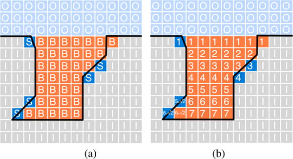
Detecting cavities using Travel Depth [CS06]: (a) each voxel is classified as i) outside the convex hull (O), ii) inside the protein surface and intersecting at least one surface atom (S), iii) inside the molecular surface (I), and iv) between the convex hull and the protein surface (B); (b) the depth is computed for each voxel in conformity with Eq. (3).

References

- [ABSC12].Al-Bluwi I, Siméon T, Cortés J. Motion planning algorithms for molecular simulations: A survey. Computer Science Review. 2012;6(4):125–143. [Google Scholar]
- [AGBT01].Armon A, Graur D, Ben-Tal N. ConSurf: an algorithmic tool for the identification of functional regions in proteins by surface mapping of phylogenetic information. Journal of Molecular Biology. 2001;307(1):447–463. doi: 10.1006/jmbi.2000.4474. [DOI] [PubMed] [Google Scholar]
- [AJL*07].Alberts B, Johnson A, Lewis J, Raff M, Roberts K, Walter P. Molecular Biology of the Cell. Garland Science; New York, USA: 2007. [Google Scholar]
- [AMA*12].Ashford P, Moss DS, Alex A, Yeap SK, Povia A, Nobeli I, Williams MA. Visualisation of variable binding pockets on protein surfaces by probabilistic analysis of related structure sets. BMC Bioinformatics. 2012;13(1):1–16. doi: 10.1186/1471-2105-13-39. [DOI] [PMC free article] [PubMed] [Google Scholar]
- [BAM*14].Benkaidali L, André F, Maouche B, Siregar P, Benyettou M, Maurel F, Petitjean M. Computing cavities, channels, pores and pockets in proteins from non spherical ligands models. Bioinformatics. 2014;30(6):792–800. doi: 10.1093/bioinformatics/btt644. [DOI] [PubMed] [Google Scholar]
- [BCG*13].Brezovsky J, Chovancova E, Gora A, Pavelka A, Biedermannova L, Damborsky J. Software tools for identification, visualization and analysis of protein tunnels and channels. Biotechnology Advances. 2013;31(1):38–49. doi: 10.1016/j.biotechadv.2012.02.002. [DOI] [PubMed] [Google Scholar]
- [BD05].Boissonnat J, Delage C. Convex hull and Voronoi diagram of additively weighted points. In: Brodal G, Leonardi S, editors. Proceedings of the 13th Annual European Conference on Algorithms. Vol. 3669. Springer Berlin Heidelberg; 2005. pp. 367–378. (Lecture Notes in Computer Science). [Google Scholar]
- [BDH96].Barber CB, Dobkin DP, Huhdanpaa H. The quickhull algorithm for convex hulls. ACM Transactions on Mathematical Software. 1996;22(4):469–483. [Google Scholar]
- [BDST04].Bajaj C, Djeu P, Siddavanahalli V, Thane A. Texmol: Interactive visual exploration of large flexible multi-component molecular complexes. Proceedings of the IEEE Conference on Visualization (IEEEVis’04); Austin, Texas, USA. October 10–15; IEEE Press; 2004. pp. 243–250. [Google Scholar]
- [BGG09].Bajaj C, Gillette A, Goswami S. Topology based selection and curation of level sets. In: Hege HC, Polthier K, Scheuermann G, editors. Topology-Based Methods in Visualization II. Springer-Verlag; 2009. pp. 45–58. (Mathematics and Visualization). [DOI] [PMC free article] [PubMed] [Google Scholar]
- [BGG*10].Bajaj C, Gillette A, Goswami S, Kwon BJ, Rivera J. Complementary space for enhanced uncertainty and dynamics visualization. In: Pascucci V, Tricoche X, Hagen H, Tierny J, editors. Topological Methods in Data Analysis and Visualization. Springer-Verlag; 2010. pp. 217–228. (Mathematics and Visualization). [Google Scholar]
- [BHH*09].Buša J, Hayryan S, Hu CK, Skřivánek J, Wu MC. Enveloping triangulation method for detecting internal cavities in proteins and algorithm for computing their surface areas and volumes. Journal of Computational Chemistry. 2009;30(3):346–357. doi: 10.1002/jcc.21060. [DOI] [PubMed] [Google Scholar]
- [BHH*10].Buša J, Hayryan S, Hu CK, Skřivánek J, Wu MC. Cave: A package for detection and quantitative analysis of internal cavities in a system of overlapping balls: Application to proteins. Computer Physics Communications. 2010;181(12):2116–2125. [Google Scholar]
- [BHHW15].Buša J, Hayryan S, Hu CK, Wu MC. Cave-CL: An OpenCL version of the package for detection and quantitative analysis of internal cavities in a system of overlapping balls: Application to proteins. Computer Physics Communications. 2015;190:224–227. [Google Scholar]
- [Bli82].Blinn JF. A generalization of algebraic surface drawing. ACM Transactions on Graphics. 1982 Jul;1(3):235–256. [Google Scholar]
- [Blu67].Blum H. A transformation for extracting new descriptors of shape. In: Wathen-Dunn W, editor. Proceedings of the Symposium on Models for the Perception of Speech and Visual Form; Boston, Massachusetts. November 11–14, 1964; MIT Press; 1967. pp. 362–380. [Google Scholar]
- [BNL03].Binkowski TA, Naghibzadeh S, Liang J. CASTp: computed atlas of surface topography of proteins. Nucleic Acids Research. 2003;31(13):3352–3355. doi: 10.1093/nar/gkg512. [DOI] [PMC free article] [PubMed] [Google Scholar]
- [Bor11].Borland D. Ambient occlusion opacity mapping for visualization of internal molecular structure. Journal of WSCG. 2011;19(1–3):17–24. [Google Scholar]
- [BS00].Brady GP, Stouten PFW. Fast prediction and visualization of protein binding pockets with PASS. Journal of Computer-Aided Molecular Design. 2000 May;14(4):383–401. doi: 10.1023/a:1008124202956. [DOI] [PubMed] [Google Scholar]
- [CCL03].Cazals F, Chazal F, Lewiner T. Molecular shape analysis based upon the Morse-Smale complex and the Connolly function. Proceedings of the 19th Annual Symposium on Computational Geometry (SCG’03); San Diego, California, USA. June 8–10; ACM Press; 2003. pp. 351–360. [Google Scholar]
- [Con83].Connolly M. Analytical molecular surface calculation. Journal of Applied Crystallography. 1983 Oct;16(5):548–558. [Google Scholar]
- [Con86].Connolly M. Measurement of protein surface shape by solid angles. Journal of Molecular Graphics. 1986;4(1):3–6. [Google Scholar]
- [CPB*12].Chovancova E, Pavelka A, Benes P, Strnad O, Brezovsky J, Kozlikova B, Gora A, Sustr V, Klvana M, Medek P, et al. CAVER 3.0: a tool for the analysis of transport pathways in dynamic protein structures. PLoS Computational Biology. 2012;8(10):e1002708:1–12. doi: 10.1371/journal.pcbi.1002708. [DOI] [PMC free article] [PubMed] [Google Scholar]
- [CPG*11].Craig IR, Pfleger C, Gohlke H, Essex JW, Spiegel K. Pocket-space maps to identify novel binding-site conformations in proteins. Journal of Chemical Information and Modeling. 2011;51(10):2666–2679. doi: 10.1021/ci200168b. [DOI] [PubMed] [Google Scholar]
- [CS06].Coleman RG, Sharp KA. Travel Depth, a new shape descriptor for macromolecules: Application to ligand binding. Journal of Molecular Biology. 2006;362(3):441–458. doi: 10.1016/j.jmb.2006.07.022. [DOI] [PubMed] [Google Scholar]
- [CS09].Coleman RG, Sharp KA. Finding and characterizing tunnels in macromolecules with application to ion channels and pores. Biophysical Journal. 2009;96(2):632–645. doi: 10.1529/biophysj.108.135970. [DOI] [PMC free article] [PubMed] [Google Scholar]
- [CS10].Coleman R, Sharp K. Protein pockets: Inventory, shape, and comparison. Journal of Chemical Information and Modeling. 2010;50(4):589–603. doi: 10.1021/ci900397t. [DOI] [PMC free article] [PubMed] [Google Scholar]
- [CVT*11].Chavent M, Vanel A, Tek A, Levy B, Robert S, Raffin B, Baaden M. GPU-accelerated atom and dynamic bond visualization using hyperballs: A unified algorithm for balls, sticks, and hyperboloids. Journal of Computational Chemistry. 2011;32(13):2924–2935. doi: 10.1002/jcc.21861. [DOI] [PubMed] [Google Scholar]
- [Czi15].Czirják G. PrinCCes: Continuity-based geometric decomposition and systematic visualization of the void repertoire of proteins. Journal of Molecular Graphics and Modelling. 2015 Nov;62:118–127. doi: 10.1016/j.jmgm.2015.09.013. [DOI] [PubMed] [Google Scholar]
- [DBG10].Dias S, Bora K, Gomes A. CUDA-based triangulations of convolution molecular surfaces. Proceedings of the 19th Acm International Symposium on High Performance Distributed Computing (HPDC’10); Chicago, Illinois, USA. June 21–25; ACM Press; 2010. pp. 531–540. [Google Scholar]
- [DCD*14].D’agostino D, Clematis A, Decherchi S, Rocchia W, Milanesi L, Merelli I. CUDA accelerated molecular surface generation. Concurrency and Computation: Practice and Experience. 2014;26(10):1819–1831. [Google Scholar]
- [DCTS93].Del Carpio C, Takahashi Y, Sasaki S. A new approach to the automatic identification of candidates for ligand receptor sites in proteins: (I). Search for pocket regions. Journal of Molecular Graphics. 1993;11(1):23–29. doi: 10.1016/0263-7855(93)85003-9. [DOI] [PubMed] [Google Scholar]
- [DdOM11].Durrant J, de Oliveira C, McCammon JA. POVME: an algorithm for measuring binding-pocket volumes. Journal of Molecular Graphics and Modelling. 2011;29(5):773–776. doi: 10.1016/j.jmgm.2010.10.007. [DOI] [PMC free article] [PubMed] [Google Scholar]
- [Del92].Delaney JS. Finding and filling protein cavities using cellular logic operations. Journal of Molecular Graphics. 1992;10(3):174–177. doi: 10.1016/0263-7855(92)80052-f. [DOI] [PubMed] [Google Scholar]
- [DG13].Dias S, Gomes A. Triangulating Molecular Surfaces on Multiple GPUs. Proceedings of the 20th European MPI Users’ Group Meeting (EuroMPI’13); Madrid, Spain. September 15–18; ACM Press; 2013. pp. 181–186. [Google Scholar]
- [DG15].Dias S, Gomes AJ. Triangulating Gaussian-like Surfaces of Molecules with Millions of Atoms. In: Rocchia W, Spagnuolo M, editors. Computational Electrostatics for Biological Applications. Springer International Publishing; 2015. pp. 177–198. [Google Scholar]
- [DG17].Dias S, Gomes A. GPU-Based Detection of Protein Cavities using Gaussian Implicit Surfaces. 2017 doi: 10.1186/s12859-017-1913-4. (submitted for publication) [DOI] [PMC free article] [PubMed] [Google Scholar]
- [DK91].Doi A, Koide A. An efficient method of triangulating equi-valued surfaces by using tetrahedral cells. IEICE Transactions on Information Systems E74-D. 1991;1:214–224. [Google Scholar]
- [DLW08].Dessailly BH, Lensink MF, Wodak SJ. LigAsite: a database of biologically relevant binding sites in proteins with known apo-structures. Nucleic Acids Research. 2008;36:D667–673. doi: 10.1093/nar/gkm839. [DOI] [PMC free article] [PubMed] [Google Scholar]
- [DNB15].Desdouits N, Nilges M, Blondel A. Principal component analysis reveals correlation of cavities evolution and functional motions in proteins. Journal of Molecular Graphics and Modelling. 2015 Feb;55:13–24. doi: 10.1016/j.jmgm.2014.10.011. [DOI] [PubMed] [Google Scholar]
- [DNJG17].Dias SE, Nguyen QT, Jorge JA, Gomes AJ. Multi-GPU-based detection of protein cavities using critical points. Future Generation Computer Systems. 2017 Feb;67:430–440. [Google Scholar]
- [Duk13].Dukka B. Structure-based methods for computational protein functional site prediction. Computational and Structural Biotechnology Journal. 2013;8(11):1–8. doi: 10.5936/csbj.201308005. [DOI] [PMC free article] [PubMed] [Google Scholar]
- [Ede95].Edelsbrunner H. The union of balls and its dual shape. Discrete & Computational Geometry. 1995;13(3):415–440. [Google Scholar]
- [Ede98].Edelsbrunner H. On the definition and the construction of pockets in macromolecules. Discrete Applied Mathematics. 1998 Nov;88(1–3):83–102. [Google Scholar]
- [EFFL95].Edelsbrunner H, Facello M, Fu P, Liang J. Measuring proteins and voids in proteins. Proceedings of the 28th Hawaii International Conference on System Sciences (HICSS’95); Maui, Hawaii. January 3–6; IEEE Press; 1995. pp. 256–264. [Google Scholar]
- [EH07].Eyrisch S, Helms V. Transient pockets on protein surfaces involved in protein-protein interaction. Journal of Medicinal Chemistry. 2007;50(15):3457–3464. doi: 10.1021/jm070095g. [DOI] [PubMed] [Google Scholar]
- [EK06].Emiris IZ, Karavelas MI. The predicates of the apollonius diagram: algorithmic analysis and implementation. Computational Geometry. 2006;33(1):18–57. [Google Scholar]
- [EKMB98].Exner T, Keil M, Moeckel G, Brickmann J. Identification of substrate channels and protein cavities. Journal of Molecular Modeling. 1998;4(10):340–343. [Google Scholar]
- [EKS83].Edelsbrunner H, Kirkpatrick DG, Seidel R. On the shape of a set of points in the plane. IEEE Transactions on Information Theory. 1983;29(4):551–559. [Google Scholar]
- [EKSX96].Ester M, Kriegel H, Sander J, Xu X. A density-based algorithm for discovering clusters in large spatial databases with noise. Proceedings of the 2nd International Conference on Knowledge Discovery and Data Mining (KDD’96); Portland, Oregon, USA. August 2–4; AAAI Press; 1996. pp. 226–231. [Google Scholar]
- [EM94].Edelsbrunner H, Mucke EP. Three-dimensional alpha shapes. ACM Transactions on Graphics. 1994;13:43–72. [Google Scholar]
- [GAGM11].Giard J, Alface PR, Gala JL, Macq B. Fast surface-based travel depth estimation algorithm for macromolecule surface shape description. IEEE/ACM Transactions on Computational Biology and Bioinformatics. 2011;8(1):59–68. doi: 10.1109/TCBB.2009.53. [DOI] [PubMed] [Google Scholar]
- [Goo85].Goodford PJ. A computational procedure for determining energetically favorable binding sites on biologically important macromolecules. Journal of Medicinal Chemistry. 1985;28(7):849–857. doi: 10.1021/jm00145a002. [DOI] [PubMed] [Google Scholar]
- [GP95].Grant JA, Pickup BT. A Gaussian Description of Molecular Shape. Journal of Physical Chemistry. 1995;99(11):3503–3510. [Google Scholar]
- [GS11].Ghersi D, Sanchez R. Beyond structural genomics: computational approaches for the identification of ligand binding sites in protein structures. Journal of Structural and Functional Genomics. 2011;12(2):109–117. doi: 10.1007/s10969-011-9110-6. [DOI] [PMC free article] [PubMed] [Google Scholar]
- [GS13].Gao M, Skolnick J. A comprehensive survey of small-molecule binding pockets in proteins. PLOS Computational Biology. 2013;9(10):1–12. doi: 10.1371/journal.pcbi.1003302. [DOI] [PMC free article] [PubMed] [Google Scholar]
- [GVJ*09].Gomes A, Voiculescu I, Jorge J, Wyvill B, Galbraith C. Implicit Curves and Surfaces: Mathematics, Data Structures and Algorithms. Springer-Verlag; London: 2009. [Google Scholar]
- [GW07].Gonzalez RC, Woods RE. Digital Image Processing. Prentice Hall; 2007. [Google Scholar]
- [Hat02].Hatcher A. Algerbraic Topology. Cambridge University Press; Cambridge, United Kingdom: 2002. [Google Scholar]
- [Hds96].Humphrey W, Dalke A, Schulten K. VMD: visual molecular dynamics. Journal of Molecular Graphics. 1996;14(1):33–38. doi: 10.1016/0263-7855(96)00018-5. [DOI] [PubMed] [Google Scholar]
- [HG08].Ho B, Gruswitz F. HOLLOW: generating accurate representations of channel and interior surfaces in molecular structures. BMC Structural Biology. 2008;8(1):49. doi: 10.1186/1472-6807-8-49. [DOI] [PMC free article] [PubMed] [Google Scholar]
- [HGVV16].Hermosilla P, Guallar V, Vinacua A, Vázquez P. High quality illustrative effects for molecular rendering. Computers & Graphics. 2016;54:113–120. [Google Scholar]
- [HLP10].Hawick K, Leist A, Playne D. Parallel graph component labelling with GPUS and CUDA. Parallel Computing. 2010;36(12):655–678. [Google Scholar]
- [HM90].Ho C, Marshall G. Cavity search: An algorithm for the isolation and display of cavity-like binding regions. Journal of Computer-Aided Molecular Design. 1990;4(4):337–354. doi: 10.1007/BF00117400. [DOI] [PubMed] [Google Scholar]
- [HOG08].Harris R, Olson AJ, Goodsell DS. Automated prediction of ligand-binding sites in proteins. Proteins: Structure, Function, and Bioinformatics. 2008;70(4):1506–1517. doi: 10.1002/prot.21645. [DOI] [PubMed] [Google Scholar]
- [HRB97].Hendlich M, Rippmann F, Barnickel G. LIGSITE: automatic and efficient detection of potential small molecule-binding sites in proteins. Journal of Molecular Graphics and Modelling. 1997;15(6):359–363. doi: 10.1016/s1093-3263(98)00002-3. [DOI] [PubMed] [Google Scholar]
- [HSAH*09].Henrich S, Salo-Ahen OMH, Huang B, Rippmann FF, Cruciani G, Wade RC. Computational approaches to identifying and characterizing protein binding sites for ligand design. Journal of Molecular Recognition. 2009;23(2):209–219. doi: 10.1002/jmr.984. [DOI] [PubMed] [Google Scholar]
- [Hua09].Huang B. Metapocket: A meta approach to improve protein ligand binding site prediction. OMICS. 2009;13(4):325–330. doi: 10.1089/omi.2009.0045. [DOI] [PubMed] [Google Scholar]
- [JKSS96].Jenkins A, Kratochvil P, Stepto R, Suter U. Glossary of basic terms in polymer science (IUPAC Recommendations 1996) Pure and Applied Chemistry. 1996;68(12):2287–2311. [Google Scholar]
- [Kaw10].Kawabata T. Detection of multiscale pockets on protein surfaces using mathematical morphology. Proteins: Structure, Function, and Bioinformatics. 2010;78(5):1195–1211. doi: 10.1002/prot.22639. [DOI] [PubMed] [Google Scholar]
- [KBE09].Krone M, Bidmon K, Ertl T. Interactive visualization of molecular surface dynamics. IEEE Transactions on Visualization and Computer Graphics. 2009;15(6):1391–1398. doi: 10.1109/TVCG.2009.157. [DOI] [PubMed] [Google Scholar]
- [KBO*82].Kuntz ID, Blaney JM, Oatley SJ, Langridge R, Ferrin TE. A geometric approach to macromolecule-ligand interactions. Journal of Molecular Biology. 1982 Oct;161(2):269–288. doi: 10.1016/0022-2836(82)90153-x. [DOI] [PubMed] [Google Scholar]
- [KC08].Kalidas Y, Chandra N. PocketDepth: A new depth based algorithm for identification of ligand binding sites in proteins. Journal of Structural Biology. 2008;161(1):31–42. doi: 10.1016/j.jsb.2007.09.005. [DOI] [PubMed] [Google Scholar]
- [KCC*08].Kim D, Cho C, Cho Y, Ryu J, Bhak J, Kim D. Pocket extraction on proteins via the Voronoi diagram of spheres. Journal of Molecular Graphics and Modelling. 2008 Apr;26(7):1104–1112. doi: 10.1016/j.jmgm.2007.10.002. [DOI] [PubMed] [Google Scholar]
- [KCK04].Kim DS, Cho Y, Kim D. Edge-tracing algorithm for Euclidean Voronoi diagram of 3D Spheres. Proceedings of the 16th Canadian Conference on Computational Geometry (CCCG’04); Montréal, Quebec, Canada. August 9–11; 2004. pp. 176–179. [Google Scholar]
- [KCKC06].Kim DS, Cho CH, Kim D, Cho Y. Recognition of docking sites on a protein using β-shape based on Voronoi diagram of atoms. Computer-Aided Design. 2006;38(5):431–443. [Google Scholar]
- [KCL*14].Kim JK, Cho Y, Laskowski RA, Ryu SE, Sugihara K, Kim DS. BetaVoid: Molecular voids via beta-complexes and Voronoi diagrams. Proteins: Structure, Function, and Bioinformatics. 2014;82(9):1829–1849. doi: 10.1002/prot.24537. [DOI] [PubMed] [Google Scholar]
- [KFR*11].Krone M, Falk M, Rehm S, Pleiss J, Ertl T. Interactive exploration of protein cavities. Computer Graphics Forum. 2011;30(3):673–682. [Google Scholar]
- [KG07].Kawabata T, Go N. Detection of pockets on protein surfaces using small and large probe spheres to find putative ligand binding sites. Proteins: Structure, Function, and Bioinformatics. 2007;68(2):516–529. doi: 10.1002/prot.21283. [DOI] [PubMed] [Google Scholar]
- [KJ94].Kleywegt G, Jones T. Detection, delineation, measurement and display of cavities in macromolecular structures. Acta Crystallographica. 1994;50(Part 2):178–185. doi: 10.1107/S0907444993011333. [DOI] [PubMed] [Google Scholar]
- [KJV83].Kirkpatrick S, G CD, Jr, Vecchi MP. Optimization by simulated annealing. Science. 1983;220(4598):671–680. doi: 10.1126/science.220.4598.671. [DOI] [PubMed] [Google Scholar]
- [KKC*11].Kim B, Kim KJ, Choi JH, Baek N, Seong JK, Choi YJ. SIGGRAPH Asia 2011 Posters. ACM Press; 2011. Finding surface atoms of a protein molecule on a GPU; pp. 32–32. [Google Scholar]
- [KKL*16].Krone M, Kozlikova B, Lindow N, Baaden M, Baum D, Parulek J, Hege HC, Viola I. Visual analysis of biomolecular cavities: State of the art. Computer Graphics Forum. 2016;35(3):527–551. [Google Scholar]
- [KKS01A].Kim DS, Kim D, Sugihara K. Voronoi diagram of a circle set from Voronoi diagram of a point set: I. Topology. Computer Aided Geometric Design. 2001;18(6):541–562. [Google Scholar]
- [KKS01B].Kim DS, Kim D, Sugihara K. Voronoi diagram of a circle set from Voronoi diagram of a point set: II. Geometry. Computer Aided Geometric Design. 2001;18(6):563–585. [Google Scholar]
- [KLKK16].Kim B, Lee JE, Kim YJ, Kim KJ. GPU accelerated finding of channels and tunnels for a protein molecule. International Journal of Parallel Programming. 2016;44(1):87–108. [Google Scholar]
- [KRH*13].Kokh DB, Richter S, Henrich S, Czodrowski P, Rippmann F, Wade RC. TRAPP: A tool for analysis of transient binding pockets in proteins. Journal of Chemical Information and Modeling. 2013;53(5):1235–1252. doi: 10.1021/ci4000294. [DOI] [PubMed] [Google Scholar]
- [KRS*13].Krone M, Reina G, Schulz C, Kulschewski T, Pleiss J, Ertl T. Interactive extraction and tracking of biomolecular surface features. Computer Graphics Forum. 2013;32(3):331–340. [Google Scholar]
- [KSK*06].Kim DS, Seo J, Kim D, Ryu J, Cho CH. Three-dimensional beta-shapes. Computer-Aided Design. 2006;38(11):1179–1191. [Google Scholar]
- [KSL*15].Kuenemann MA, Sperandio O, Labbé CM, Lagorce D, Miteva MA, Villoutreix BO. In silico design of low molecular weight protein-protein interaction inhibitors: Overall concept and recent advances. Progress in Biophysics and Molecular Biology. 2015;119(1):20–32. doi: 10.1016/j.pbiomolbio.2015.02.006. [DOI] [PubMed] [Google Scholar]
- [KSS*14].Kozlikova B, Sebestova E, Sustr V, Brezovsky J, Strnad O, Daniel L, Bednar D, Pavelka A, Manak M, Bezdeka M, et al. CAVER Analyst 1.0: graphic tool for interactive visualization and analysis of tunnels and channels in protein structures. Bioinformatics. 2014;30(18):2684–2685. doi: 10.1093/bioinformatics/btu364. [DOI] [PubMed] [Google Scholar]
- [Kub06].Kubinyi H. Chemogenomics in drug discovery. In: Jaroch S, Weinmann H, editors. Chemical Genomics: Small Molecule Probes to Study Cellular Function. Vol. 58. Springer-Verlag; 2006. pp. 1–19. (Ernst Schering Research Foundation Workshop Series). [DOI] [PubMed] [Google Scholar]
- [Las95].Laskowski RA. SURFNET: A program for visualizing molecular surfaces, cavities, and intermolecular interactions. Journal of Molecular Graphics. 1995;13(5):323–330. doi: 10.1016/0263-7855(95)00073-9. [DOI] [PubMed] [Google Scholar]
- [Lay82].Lay SR. Convex Sets and Their Applications. Dover Publications, Inc; Mineola, New York, USA: 1982. [Google Scholar]
- [LB92].Levitt DG, Banaszak LJ. POCKET: A computer graphic method for identifying and displaying protein cavities and their surrounding amino acids. Journal of Molecular Graphics. 1992;10(4):229–234. doi: 10.1016/0263-7855(92)80074-n. [DOI] [PubMed] [Google Scholar]
- [LBBH13].Lindow N, Baum D, Bondar AN, Hege HC. Exploring cavity dynamics in biomolecular systems. BMC Bioinformatics. 2013;14(Suppl. 19):S5:1–12. doi: 10.1186/1471-2105-14-S19-S5. [DOI] [PMC free article] [PubMed] [Google Scholar]
- [LBH11].Lindow N, Baum D, Hege HC. Voronoi-based extraction and visualization of molecular paths. IEEE Transactions on Visualization and Computer Graphics. 2011;17(12):2025–2034. doi: 10.1109/TVCG.2011.259. [DOI] [PubMed] [Google Scholar]
- [LBH14].Lindow N, Baum D, Hege HC. Ligand excluded surface: A new type of molecular surface. IEEE Transactions on Visualization and Computer Graphics. 2014;20(12):2486–2495. doi: 10.1109/TVCG.2014.2346404. [DOI] [PubMed] [Google Scholar]
- [LCC*15].Laurent B, Chavent M, Cragnolini T, Dahl ACE, Pasquali S, Derreumaux P, Sansom MS, Baaden M. Epock: rapid analysis of protein pocket dynamics. Bioinformatics. 2015;31(9):1478–1480. doi: 10.1093/bioinformatics/btu822. [DOI] [PMC free article] [PubMed] [Google Scholar]
- [LGST09].Le Guilloux V, Schmidtke P, Tuffery P. Fpocket: an open source platform for ligand pocket detection. BMC Bioinformatics. 2009 Dec;10(1):1–11. doi: 10.1186/1471-2105-10-168. [DOI] [PMC free article] [PubMed] [Google Scholar]
- [LJ05].Laurie ATR, Jackson RM. Q-SiteFinder: an energy-based method for the prediction of protein-ligand binding sites. Bioinformatics. 2005;21(9):1908–1916. doi: 10.1093/bioinformatics/bti315. [DOI] [PubMed] [Google Scholar]
- [LJ06].Laurie AT, Jackson RM. Methods for the prediction of protein-ligand binding sites for structure-based drug design and virtual ligand screening. Current Protein and Peptide Science. 2006 Oct;7(5):395–406. doi: 10.2174/138920306778559386. [DOI] [PubMed] [Google Scholar]
- [LLNW14].Li H, Leung KS, Nakane T, Wong MH. iview: an interactive WebGL visualizer for protein-ligand complex. BMC Bioinformatics. 2014;15(1):56. doi: 10.1186/1471-2105-15-56. [DOI] [PMC free article] [PubMed] [Google Scholar]
- [LLST96].Laskowski RA, Luscombe N, Swindells MB, Thornton JM. Protein clefts in molecular recognition and function. Protein Science. 1996;5(12):2438–2452. doi: 10.1002/pro.5560051206. [DOI] [PMC free article] [PubMed] [Google Scholar]
- [LPFL08].Loewenstein Y, Portugaly E, Fromer M, Linial M. Efficient algorithms for accurate hierarchical clustering of huge datasets: tackling the entire protein space. Bioinformatics. 2008;24(13):i41–i49. doi: 10.1093/bioinformatics/btn174. [DOI] [PMC free article] [PubMed] [Google Scholar]
- [LR71].Lee B, Richards F. The interpretation of protein structures: Estimation of static accessibility. Journal of Molecular Biology. 1971 Feb;55(3):379–380. doi: 10.1016/0022-2836(71)90324-x. [DOI] [PubMed] [Google Scholar]
- [LS94].Lemieux RU, Spohr U. How emil fischer was led to the lock and key concept for enzyme specificity. Advances in Carbohydrate Chemistry and Biochemistry. 1994;50:1–20. [PubMed] [Google Scholar]
- [LTA*08].Li B, Turuvekere S, Agrawal M, La D, Ramani K, Kihara D. Characterization of local geometry of protein surfaces with the visibility criterion. Proteins: Structure, Function, and Bioinformatics. 2008;71(2):670–683. doi: 10.1002/prot.21732. [DOI] [PubMed] [Google Scholar]
- [LWE98].Liang J, Woodward C, Edelsbrunner H. Anatomy of protein pockets and cavities: Measurement of binding site geometry and implications for ligand design. Protein Science. 1998;7(9):1884–1897. doi: 10.1002/pro.5560070905. [DOI] [PMC free article] [PubMed] [Google Scholar]
- [LWP*13].Lo YT, Wang HW, Pai TW, Tzou WS, Hsu HH, Chang HT. Protein-ligand binding region prediction (PLB-SAVE) based on geometric features and Cuda acceleration. BMCBioinformatics. 2013;14(Suppl 4) doi: 10.1186/1471-2105-14-S4-S4. [DOI] [PMC free article] [PubMed] [Google Scholar]
- [Mat75].Matheron G. Random sets and integral geometry. John Wiley & Sons, Inc; 1975. [Google Scholar]
- [MBS07].Medek P, Beneš P, Sochor J. Computation of tunnels in protein molecules using delaunay triangulation. Journal of WSCG. 2007:107–114. Václav Skala-UNION Agency. [Google Scholar]
- [MBS08].Medek P, Beneš P, Sochor J. Proceedings of the Tenth IASTED International Conference on Computer Graphics and Imaging. ACTA Press; 2008. Multicriteria tunnel computation; pp. 160–164. [Google Scholar]
- [MD95].Masuya M, Doi J. Detection and geometric modeling of molecular surfaces and cavities using digital mathematical morphology operations. Journal of Molecular Graphics and Modelling. 1995;13(6):331–336. doi: 10.1016/0263-7855(95)00071-2. [DOI] [PubMed] [Google Scholar]
- [MDH*10].Meyer T, D’abramo M, Hospital A, Rueda M, Ferrer-Costa C, Pérez A, Carrillo O, Camps J, Fenollosa C, Repchevsky D, Gelpí JL, Orozco M. MoDEL (Molecular Dynamics Extended Library): A database of atomistic molecular dynamics trajectories. Structure. 2010;18(11):1399–1409. doi: 10.1016/j.str.2010.07.013. [DOI] [PubMed] [Google Scholar]
- [MKE01].Mitchell JC, Kerr R, Eyck LFT. Rapid atomic density methods for molecular shape characterization. Journal of Molecular Graphics and Modelling. 2001;19(3–4):325–330. doi: 10.1016/s1093-3263(00)00079-6. [DOI] [PubMed] [Google Scholar]
- [MPK*12].Metz A, Pfleger C, Kopitz H, Pfeiffer-Marek S, Baringhaus KH, Gohlke H. Hot spots and transient pockets: Predicting the determinants of small-molecule binding to a protein-protein interface. Journal of Chemical Information and Modeling. 2012;52(1):120–133. doi: 10.1021/ci200322s. [DOI] [PubMed] [Google Scholar]
- [MRR*53].Metropolis N, Rosenbluth AW, Rosenbluth MN, Teller AH, Teller E. Equation of state calculations by fast computing machines. The Journal of Chemical Physics. 1953;21(6):1087–1092. [Google Scholar]
- [NH06].Nayal M, Honig B. On the nature of cavities on protein surfaces: Application to the identification of drug-binding sites. Proteins. 2006 Feb;63(4):892–906. doi: 10.1002/prot.20897. [DOI] [PubMed] [Google Scholar]
- [NSH91].Nicholls A, Sharp K, Honig B. Protein folding and association: insights from the interfacial and thermodynamic properties of hydrocarbons. Proteins. 1991;11(4):281–296. doi: 10.1002/prot.340110407. [DOI] [PubMed] [Google Scholar]
- [NWB*06].Natarajan V, Wang Y, Bremer PT, Pascucci V, Hamann B. Segmenting molecular surfaces. Computer Aided Geometric Design. 2006;23(6):495–509. [Google Scholar]
- [OFH*14].Oliveira SH, Ferraz FA, Honorato RV, Xavier-Neto J, Sobreira TJ, de Oliveira PS. KVFinder: steered identification of protein cavities as a PyMOL plugin. BMC Bioinformatics. 2014;15(197):1–8. doi: 10.1186/1471-2105-15-197. [DOI] [PMC free article] [PubMed] [Google Scholar]
- [OMV11].Olechnovič K, Margelevičius M, Venclovas Č. Voroprot: an interactive tool for the analysis and visualization of complex geometric features of protein structure. Bioinformatics. 2011;27(5):723–724. doi: 10.1093/bioinformatics/btq720. [DOI] [PubMed] [Google Scholar]
- [PB99].Pettit FK, Bowie JU. Protein surface roughness and small molecular binding sites. Journal of Molecular Biology. 1999;285(4):1377–1382. doi: 10.1006/jmbi.1998.2411. [DOI] [PubMed] [Google Scholar]
- [PBM*02].Pupko T, Bell RE, Mayrose I, Glaser F, Ben-Tal N. Rate4site: an algorithmic tool for the identification of functional regions in proteins by surface mapping of evolutionary determinants within their homologues. Bioinformatics. 2002;18:S71–S77. doi: 10.1093/bioinformatics/18.suppl_1.s71. [DOI] [PubMed] [Google Scholar]
- [PCMT09].Pellegrini-Calace M, Maiwald T, Thornton JM. Porewalker: a novel tool for the identification and characterization of channels in transmembrane proteins from their three-dimensional structure. PLoS Comput Biol. 2009;5(7):e1000440. doi: 10.1371/journal.pcbi.1000440. [DOI] [PMC free article] [PubMed] [Google Scholar]
- [PEG*14].Paramo T, East A, Garzón D, Ulmschneider MB, Bond PJ. Efficient characterization of protein cavities within molecular simulation trajectories: trj_cavity. Journal of Chemical Theory and Computation. 2014;10(5):2151–2164. doi: 10.1021/ct401098b. [DOI] [PubMed] [Google Scholar]
- [PFF96].Peters KP, Fauck J, Frommel C. The automatic search for ligand binding sites in proteins of known three-dimensional structure using only geometric criteria. Journal of Molecular Biology. 1996;256(1):201–213. doi: 10.1006/jmbi.1996.0077. [DOI] [PubMed] [Google Scholar]
- [PGD*10].Phillips M, Georgiev I, Dehof AK, Nickels S, Marsalek L, Lenhof HP, Hildebrandt A, Slusallek P. Parallel & Distributed Processing, Workshops and Phd Forum (Ipdpsw), 2010, IEEE International Symposium on. IEEE; 2010. Measuring properties of molecular surfaces using ray casting; pp. 1–7. [Google Scholar]
- [PGH*04].Pettersen EF, Goddard TD, Huang CC, Couch GS, Greenblatt DM, Meng EC, Ferrin TE. Ucsf chimeraâĂŤa visualization system for exploratory research and analysis. Journal of computational chemistry. 2004;25(13):1605–1612. doi: 10.1002/jcc.20084. [DOI] [PubMed] [Google Scholar]
- [PKKO07].Petřek M, Košinová P, Koča J, Otyepka M. Mole: a voronoi diagram-based explorer of molecular channels, pores, and tunnels. Structure. 2007;15(11):1357–1363. doi: 10.1016/j.str.2007.10.007. [DOI] [PubMed] [Google Scholar]
- [POB*06].Petřek M, Otyepka M, Banáš P, Košinová P, Koča J, Damborskỳ J. CAVER: a new tool to explore routes from protein clefts, pockets and cavities. BMC Bioinformatics. 2006;7(316):1–9. doi: 10.1186/1471-2105-7-316. [DOI] [PMC free article] [PubMed] [Google Scholar]
- [PPG10].Patrick Pfeffer, Fober THEGK. Garlig: a fully automated tool for subset selection of large fragment spaces via a self-adaptive genetic algorithm. Journal of chemical information and modeling. 2010;50(9):1644–1659. doi: 10.1021/ci9003305. [DOI] [PubMed] [Google Scholar]
- [Pro14].Prošková J. Description of protein secondary structure using dual quaternions. Journal of Molecular Structure. 2014 Nov;1076:89–93. [Google Scholar]
- [PRV13].Parulek J, Ropinski T, Viola I. Proceedings of The 29th Spring Conference on Computer Graphics. ACM; 2013. Seamless visual abstraction of molecular surfaces; pp. 107–114. [Google Scholar]
- [PSA*91].Pedersen T, Sigurskjold B, Andersen K, Kjaer M, Poulsen F, Dobson C, Redfield C. A nuclear magnetic resonance study of the hydrogen-exchange behaviour of lysozyme in crystals and solution. Journal of Molecular Biology. 1991;218(2):413–426. doi: 10.1016/0022-2836(91)90722-i. [DOI] [PubMed] [Google Scholar]
- [PSM*10].Pérot S, Sperandio O, Miteva MA, Camproux AC, Villoutreix BO, et al. Druggable pockets and binding site centric chemical space: a paradigm shift in drug discovery. Drug Discovery Today. 2010;15(15–16):656–667. doi: 10.1016/j.drudis.2010.05.015. [DOI] [PubMed] [Google Scholar]
- [PTRV12].Parulek J, Turkay C, Reuter N, Viola I. Proceedings of the 2012 IEEE Symposium on Biological Data Visualization (BioVis’2012) IEEE Press; Oct, 2012. Implicit surfaces for interactive graph based cavity analysis of molecular simulations; pp. 115–122. [Google Scholar]
- [PTRV13].Parulek J, Turkay C, Reuter N, Viola I. Visual cavity analysis in molecular simulations. BMC Bioinformatics. 2013;14(Suppl 19):S4. doi: 10.1186/1471-2105-14-S19-S4. [DOI] [PMC free article] [PubMed] [Google Scholar]
- [Ric77].Richards F. Areas, Volumes, Packing, and Protein Structure. Annual Review of Biophysics and Bioengineering. 1977 Feb;6(3):151–176. doi: 10.1146/annurev.bb.06.060177.001055. [DOI] [PubMed] [Google Scholar]
- [RK11].Raunest M, Kandt C. dxtuber: Detecting protein cavities, tunnels and clefts based on protein and solvent dynamics. Journal of Molecular Graphics and Modelling. 2011;29(7):895–905. doi: 10.1016/j.jmgm.2011.02.003. [DOI] [PubMed] [Google Scholar]
- [RTC*13].Ribeiro JV, Tamames JA, Cerqueira NM, Fernandes PA, Ramos MJ. Volarea–a bioinformatics tool to calculate the surface area and the volume of molecular systems. Chemical Biology and Drug Design. 2013;82(6):743–755. doi: 10.1111/cbdd.12197. [DOI] [PubMed] [Google Scholar]
- [Sb06].Sohn B, Bajaj C. Time-varying contour topology. IEEE Transactions on Visualization and Computer Graphics. 2006;12(1):14–25. doi: 10.1109/TVCG.2006.16. [DOI] [PMC free article] [PubMed] [Google Scholar]
- [Sbclb11].Schmidtke P, Bidon-Chanal A, Luque FJ, Barril X. MDpocket: open-source cavity detection and characterization on molecular dynamics trajectories. Bioinformatics. 2011;27(23):3276–3285. doi: 10.1093/bioinformatics/btr550. [DOI] [PubMed] [Google Scholar]
- [SDP*13].Sridharamurthy R, Doraiswamy H, Patel S, Varadarajan R, Natarajan V. Proceedings of the EuroVis - Short Papers. Leipzig, Germany: Eurographics Association; 2013. Extraction of Robust Voids and Pockets in Proteins; pp. 67–71. [Google Scholar]
- [Ser84].Serra J. Image Analysis and Mathematical Morphology. Image Analysis & Mathematical Morphology. Academic Press; 1984. [Google Scholar]
- [SGW93].Smart OS, Goodfellow JM, Wallace B. The pore dimensions of gramicidin A. Biophysical Journal. 1993;65(6):2455–2460. doi: 10.1016/S0006-3495(93)81293-1. [DOI] [PMC free article] [PubMed] [Google Scholar]
- [SHB16].Sonka M, Hlavac V, Boyle R. Image Processing, Analysis, and Machine Vision. 4th. Cengage Learning; 2016. [Google Scholar]
- [SIM03].Simonson T. Electrostatics and dynamics of proteins. Reports of Progress in Physics. 2003;66:737–787. [Google Scholar]
- [SK97].Saff E, Kuijlaars A. Distributing many points on a sphere. The Mathematical Intelligencer. 1997;19(1):5–11. [Google Scholar]
- [SNW*96].Smart OS, Neduvelil JG, Wang X, Wallace B, Sansom MS. HOLE: A program for the analysis of the pore dimensions of ion channel structural models. Journal of Molecular Graphics. 1996;14(6):354–360. doi: 10.1016/s0263-7855(97)00009-x. [DOI] [PubMed] [Google Scholar]
- [SOS96].Sanner M, Olson A, Spehner J. Reduced surface: an efficient way to compute molecular surfaces. Biopolymers. 1996;38(3):305–320. doi: 10.1002/(SICI)1097-0282(199603)38:3%3C305::AID-BIP4%3E3.0.CO;2-Y. [DOI] [PubMed] [Google Scholar]
- [SSE*10].Schmidtke P, Souaille C, Estienne F, Baurin N, Kroemer RT. Large-scale comparison of four binding site detection algorithms. Journal of Chemical Information and Modeling. 2010;50(12):2191–2200. doi: 10.1021/ci1000289. [DOI] [PubMed] [Google Scholar]
- [SSVB*13].Sehnal D, Svobodová Vařeková R, Berka K, Pravda L, Navrátilová V, Banáš P, Ionescu CM, Otyepka M, Koča J. MOLE 2.0: advanced approach for analysis of biomacromolecular channels. Journal of Cheminformatics. 2013;5(1):39. doi: 10.1186/1758-2946-5-39. [DOI] [PMC free article] [PubMed] [Google Scholar]
- [SZ12].Schneider S, Zacharias M. Combining geometric pocket detection and desolvation properties to detect putative ligand binding sites on proteins. Journal of Structural Biology. 2012;180(3):546–550. doi: 10.1016/j.jsb.2012.09.010. [DOI] [PubMed] [Google Scholar]
- [TDCL09].Tseng YY, Dupree C, Chen ZJ, Li WH. Split-pocket: identification of protein functional surfaces and characterization of their spatial patterns. Nucleic Acids Research. 2009;37:W384–W389. doi: 10.1093/nar/gkp308. [DOI] [PMC free article] [PubMed] [Google Scholar]
- [TK10].Tripathi A, Kellogg GE. A novel and efficient tool for locating and characterizing protein cavities and binding sites. Proteins: Structure, Function, and Bioinformatics. 2010;78(4):825–842. doi: 10.1002/prot.22608. [DOI] [PMC free article] [PubMed] [Google Scholar]
- [TPS12].Tanner DE, Phillips JC, Schulten K. GPU/CPU algorithm for generalized born/solvent-accessible surface area implicit solvent calculations. Journal of Chemical Theory and Computation. 2012;8(7):2521–2530. doi: 10.1021/ct3003089. [DOI] [PMC free article] [PubMed] [Google Scholar]
- [TU10].Till MS, Ullmann GM. Mcvol-a program for calculating protein volumes and identifying cavities by a monte carlo algorithm. Journal of molecular modeling. 2010;16(3):419–429. doi: 10.1007/s00894-009-0541-y. [DOI] [PubMed] [Google Scholar]
- [VG10].Voss NR, Gerstein M. 3V: cavity, channel and cleft volume calculator and extractor. Nucleic Acids Research. 2010;38:W555–W562. doi: 10.1093/nar/gkq395. [DOI] [PMC free article] [PubMed] [Google Scholar]
- [VGGR10].Volkamer A, Griewel A, Grombacher T, Rarey M. Analyzing the Topology of Active Sites: On the Prediction of Pockets and Subpockets. Journal of Chemical Information and Modeling. 2010 Nov;50(11):2041–2052. doi: 10.1021/ci100241y. [DOI] [PubMed] [Google Scholar]
- [VKV*89].Voorintholt R, Kosters M, Vegter G, Vriend G, Hol W. A very fast program for visualizing protein surfaces, channels and cavities. Journal of Molecular Graphics. 1989;7(4):243–245. doi: 10.1016/0263-7855(89)80010-4. [DOI] [PubMed] [Google Scholar]
- [Whi97].Whitley DC. Van der waals surface graphs and molecular shape. Journal of Mathematical Chemistry. 1997;23(3–4):377–397. [Google Scholar]
- [Whi05].Whitford D. Proteins: Structure and Function. 1st. John Wiley & Sons, Ltd; 2005. [Google Scholar]
- [WM97].Wilkinson A, Mcnaught A. IUPAC Compendium of Chemical Terminology. 1997. (the “Gold Book”) [Google Scholar]
- [WPS07].Weisel M, Proschak E, Schneider G. PocketPicker: analysis of ligand binding-sites with shape descriptors. Chemistry Central Journal. 2007;1(1):1–17. doi: 10.1186/1752-153X-1-7. [DOI] [PMC free article] [PubMed] [Google Scholar]
- [XB07].Xie L, Bourne P. A robust and efficient algorithm for the shape description of protein structures and its application in predicting ligand binding sites. BMC Bioinformatics. 2007;8(Suppl 4) doi: 10.1186/1471-2105-8-S4-S9. [DOI] [PMC free article] [PubMed] [Google Scholar]
- [YFW*08].Yaffe E, Fishelovitch D, Wolfson HJ, Halperin D, Nussinov R. MolAxis: efficient and accurate identification of channels in macromolecules. Proteins. 2008 Oct;73(1):72–86. doi: 10.1002/prot.22052. [DOI] [PMC free article] [PubMed] [Google Scholar]
- [YZTY10].Yu J, Zhou Y, Tanaka I, Yao M. Roll: a new algorithm for the detection of protein pockets and cavities with a rolling probe sphere. Bioinformatics. 2010;26(1):46–52. doi: 10.1093/bioinformatics/btp599. [DOI] [PubMed] [Google Scholar]
- [Zb07].Zhang X, Bajaj C. Extraction, quantification and visualization of protein pockets. Comput Syst Bioinformatics Conf. 2007;6:275–286. [PubMed] [Google Scholar]
- [ZGWW12].Zheng X, Gan L, Wang E, Wang J. Pocket-based drug design: Exploring pocket space. The AAPS Journal. 2012;15(1):228–241. doi: 10.1208/s12248-012-9426-6. [DOI] [PMC free article] [PubMed] [Google Scholar]
- [ZLL*11].Zhang Z, Li Y, Lin B, Schroeder M, Huang B. Identification of cavities on protein surface using multiple computational approaches for drug binding site prediction. Bioinformatics. 2011;27(15):2083–2088. doi: 10.1093/bioinformatics/btr331. [DOI] [PubMed] [Google Scholar]
- [ZP11].Zhu H, Pisabarro MT. MSpocket: an orientation-independent algorithm for the detection of ligand binding pockets. Bioinformatics. 2011;27(3):351–358. doi: 10.1093/bioinformatics/btq672. [DOI] [PubMed] [Google Scholar]