Harmonization of cortical thickness measurements across scanners and sites

Abstract

With the proliferation of multi-site neuroimaging studies, there is a greater need for handling non-biological variance introduced by differences in MRI scanners and acquisition protocols. Such unwanted sources of variation, which we refer to as “scanner effects”, can hinder the detection of imaging features associated with clinical covariates of interest and cause spurious findings. In this paper, we investigate scanner effects in two large multi-site studies on cortical thickness measurements across a total of 11 scanners. We propose a set of tools for visualizing and identifying scanner effects that are generalizable to other modalities. We then propose to use ComBat, a technique adopted from the genomics literature and recently applied to diffusion tensor imaging data, to combine and harmonize cortical thickness values across scanners. We show that ComBat removes unwanted sources of scan variability while simultaneously increasing the power and reproducibility of subsequent statistical analyses. We also show that ComBat is useful for combining imaging data with the goal of studying life-span trajectories in the brain.

1 Introduction

Large-scale efforts aimed at collecting diverse neuroimaging datasets for dissemination and sharing are rapidly growing in number and scale [Di Martino et al., 2014, Keator et al., 2013, Mennes et al., 2013]. Having multiple scanning sites is necessary in large-scale studies due to logistical issues and geographic variability in subject populations [Van Horn and Toga, 2009]. However, a major drawback of combining neuroimaging studies across sites is the introduction of non-biological sources of variability to the data, typically related to image acquisition protocol and hardware.

Properties of MRI scanners such as field strength, manufacturer, gradient nonlinearity, subject positioning, and longitudinal drift have been long understood to increase bias and variance in the measurement of brain volume changes [Takao et al., 2011], regional cortical thickness [Han et al., 2006], voxel-based morphometry [Takao et al., 2014], and structural, functional, and diffusion images in general [Jovicich et al., 2006, Takao et al., 2011]. Such unwanted sources of bias and variability are typically included as confound variables in the analysis of neuroimaging data. Recent work has suggested that standard methods for including confound variables for the prediction of an outcome using neuroimaging data perform no better than baseline models which ignore confounding [Rao et al., 2017]. Furthermore, non-biological confounders typically have a priori unpredictable effects, thus compromising consistency and reproducibility of the downstream analyses across studies. This suggests that non-biological sources of variability should be handled differently. Similar to batch effects in genomics (see Leek et al. [2010] for a review of batch effects), we use the term scanner effects in neuroimaging to refer to unwanted variation that is (1) non-biological in nature and (2) associated with differential scanning equipment or parameter configurations. Because different imaging sites use different physical scanners, site effects are one example of scanner effects.

Recently, ComBat [Johnson et al., 2007], a batch-effect correction tool commonly used in genomics, has been adapted for the modeling and removal of site effects in multi-site DTI studies [Fortin et al., 2017]. ComBat was found to be an effective harmonization technique that both removes unwanted variation associated with site and preserves biological associations in the data.

In this paper, we propose to use ComBat for harmonizing cortical thickness measurements obtained from multiple sites. We investigate this in region-level cortical thickness measurements in two large multi-site datasets: the Establishing Moderators and Biosignatures of Antidepressant Response in Clinical care study (EMBARC) [Trivedi et al., 2016], a multi-center study with 4 sites, and the Vascular Depression: Longitudinal Changes (VDLC) study, which was conducted at Washington University in St. Louis and Duke University and used a total of 7 scanners. We first propose a set of tools for the visualization and identification of site effects that are generalizable to other modalities. We then harmonize the data using ComBat, and compare to two other harmonization methods: residuals and phenotype-adjusted residuals. We show that Combat is successful at removing scanner and site effects, while preserving the variability associated with biology. We also show that ComBat can be used to combine datasets across multiple sites for the study of life-span trajectories.

2 Methods

2.1 Data and Preprocessing

EMBARC dataset

The EMBARC study aims to identify moderators and mediators of antidepressant response in adult patients with Major Depressive Disorder [Trivedi et al., 2016, Webb et al., 2016]. The dataset used for our analysis includes structural images, demographic variables and clinical variables. Participants were 200 unmedicated depressed individuals with Major depressive disorder and 40 healthy individuals recruited for EMBARC. Subjects were 18–65 years old, had to report age of depression onset before age 30 and had to be fluent in English. Clinical variables included the Hamilton Depression Rating Scale (HAMD) [Hamilton, 1960], the Mood and Anxiety Symptom Questionnaire (MASQ) [Watson and Clark, 1991], the Snaith-Hamilton Pleasure Scale [Snaith et al., 1995], the Spielberger State-Trait Anxiety Inventory (STAI) [Spielberger, 1983] and the Quick Inventory for Depression Symptomatology (QIDS) depression score [Rush et al., 2003].

The scans were acquired at four different imaging sites, with acquisition protocols described in Greenberg et al. [2015]. The four sites were Columbia University (CU), University of Texas Southwestern (TX), Massachusetts General Hospital (MG) and the University of Michigan (UM). All of the sites used 3T scanners, however the manufacturer differed from site to site: UM used a Philips Ingenia 3T scanner, TX used a Philips Achieva 3T scanner, MG used a Siemens TIM Trio 3T scanner and CU used a GE SIGNA HDx 3T scanner. Imaging parameters for each scanner are described in Greenberg et al. [2015]. Participants with excessive motion (> 4 mm), low slice signal-to-noise ratio (<80), and severe slice artifacts were excluded from the study, leaving us with a final baseline dataset of 187 subjects.

VDLC dataset

The Vascular Depression: Longitudinal Changes (VDLC) study aims to study the longitudinal effect of vascular disease in the pathogenesis of late-life depression (LLD) [Barch et al., 2012, Mettenburg et al., 2012]. Participants were 117 individuals affected by LLD and 59 healthy controls, for a total of 236 participants. Participants were 58–95 years old. For the purpose of investigating site effects, we only considered one time point for each participant; we retained the scan from the last visit. Scans were acquired at two sites: Duke University and Washington University in St. Louis, across 7 different scanners described in Table 2.

Table 2. Description of the scanning parameters.

CU: Columbia University; MG: Massachusetts General Hospital; TX: University of Texas Southwestern; UM: University of Michigan; Duke: Duke University; WashU: Washington University in St. Louis.

	Location	Manufacturer	Platform	Field (T)	TR (ms)	TE (ms)	Angle (°)	ST (mm)
EMBARC study
CU	CU	GE	SIGNA HDx	3	6	2.4	9	1
MG	MG	Siemens	TIM Trio	3	2300	2.54	9	1
TX	TX	Philips	Achieva	3	2100	3.7	12	1
UM	UM	Philips	Ingenia	3	8.2	3.7	12	1
VDLC study
W_Sonata_A	WashU	Siemens	Sonata	1.5	{500,1900}	{3.93,17}	{8,90}	{1,2,3,5}
W_Sonata_B	WashU	Siemens	Sonata	1.5	{500,1900}	{3.93,17}	{8,90}	{1,2,3,5}
W_TIMTrio_A	WashU	Siemens	TIM Trio	3	2400	{3.13,3.16}	8	1
W_TIMTrio_B	WashU	Siemens	TIM Trio	3	2400	3.13	8	1
D_TIMTrio_A	Duke	Siemens	TIM Trio	3	{2300,2400}	{3.19,3.43}	{8,12}	1
D_TIMTrio_B	Duke	Siemens	TIM Trio	3	2300	{2.98,3.43}	12	1
D_SIGNA	Duke	GE	SIGNA Excite	1.5	8.3	3.3	20	1.2

2.2 Extraction of cortical thickness measurements

For the extraction of the cortical thickness measurements, we ran the ANTs cortical thickness (CT) pipeline which has been shown to provide accurate and robust cortical thickness measurements [Tustison et al., 2014] on each dataset separately. We analyzed VDLC dataset in early 2016 and the EMBARC in late 2014, each using contemporaneous installations of ANTs compiled from source. The ANTs CT pipeline that we describe below, requires a population template for registration and prior knowledge of the different tissues. We used an average labeled template previously constructed from a subset of 35 participants from the Open Access Series of Imaging Studies (OASIS) [Marcus et al., 2007]. The participants’ age ranges from 19 to 90 years old. All subjects were healthy, except one who was diagnosed with mild dementia. For each image, a manual brain segmentation was performed by Neuromorphometrics, Inc. (http://Neuromorphometrics.com/) using the brainCOLOR labeling protocol. Multi-Atlas Label Fusion (MALF, [Wang et al., 2013b]) was used to create the consensus labels for the average template, for a total of 134 labelled regions, from which 98 are part of the cortex. We provide the list of the 98 cortical regions in Supplementary Table 1. We note that the population template is publicly available on Figshare (https://figshare.com/articles/ANTs_ANTsR_Brain_Templates/915436).

The ANTs CT extraction pipeline starts by performing a N4 bias field correction [Tustison et al., 2010] to minimize field inhomogeneity effects, and then performs brain extraction using a hybrid registration/segmentation method described in Tustison et al. [2014]. For each participant, a tissue segmentation is performed using Atropos [Avants et al., 2011] to create six tissue masks: cerebrospinal fluid (CSF), grey matter (GM), white matter (WM), deep gray matter, brain stem, and cerebellum. Atropos allows prior knowledge to guide the segmentation algorithm, and we used the labels from the OASIS population template as priors. Cortical thickness measurements are then estimated using the DiReCT algorithm [Das et al., 2009]. Briefly, the DiReCT method estimates the GM/WM interface and the GM/CSF interface and computes a diffeomorphic mapping between the two interfaces, from which thickness is derived. We note that this is performed in native space and no correction for total brain volume was applied.

In the EMBARC data, we built a study-specific population template and performed pseudo-geodesic joint label fusion by combining precomputed warps from the OASIS atlases to the EMBARC template with warps from the average template to each subject. The atlases and labels were warped to subject space and input to joint label fusion [Wang et al., 2013a]. The fused labels were masked with the subject’s gray-matter segmentation image, which is the domain over which thickness is computed in the ANTs pipeline. For the VLDC data, given the heterogeneity of the acquisition parameters we used the OASIS population template and directly propagated the consensus labels from the OASIS template to each image with nearest neighbor interpolation. For both datasets, mean thickness was computed for each of the 98 cortical regions in the subject space, these were in turn averaged to produce whole-brain mean cortical thickness.

After the processing steps described above, we performed manual quality control of the images by visual inspection. We specifically looked at the quality of the skull stripping, registration and mesh reconstruction. We flagged a few images distributed across the sites that appeared to be abnormal, but we did not see differences in the cortical thickness measurements as compared to other images. We note that the ANTs pipeline has been shown to perform exceptionally well for registration [Klein et al., 2009] as well as cortical thickness measurement in terms of minimal failure rate, higher repeatability, and improved predictive performance in thousands of images even compared to the state-of-the-art FreeSurfer [Tustison et al., 2014].

2.3 Harmonization procedures

For the removal of site effects, we compare three different harmonization procedures: (1) Removal of site effects using linear regression without adjusting for biological covariates. We refer to the method as Residuals; (2) Removal of site effects using linear regression, adjusting for known covariates. We refer to the method as Adjusted Residuals; (3) Removal of site effects using ComBat [Johnson et al., 2007]. We also compare the three methods to the absence of harmonization, that we refer to as Raw. We describe below the different harmonization techniques.

To describe each of these different methods, we use the following notation: let y_ijv be the n × 1 vector of cortical thickness measurement for imaging site i, for participant j and feature v, for a total of (k + 1) sites, n participants and V features. Depending on the cortical thickness modality, the features can either be ROIs, vertices or voxels. Furthermore, let X be the p × n matrix of biological covariates of interests, and let Z be the k × n matrix of site indicators (deviations from a baseline site).

2.3.1 Residuals harmonization

The residuals harmonization method adjusts the images for site effects using linear regression. It does not take into account the potential confounding between the site variables and the biological covariates of interest in the study. The regression model can be written as

$$y_{ij\nu }={\alpha }_{\nu }+{\mathbf{Z}}_{ij}^T{\theta }_{\nu }+{\epsilon }_{ij\nu }$$ (1)

where α_v is the average cortical thickness for the reference site for feature v and where θ_v is the k × 1 vector of the coefficients associated with Z for feature v. We assume that the residual terms ε_ijv have mean 0. For each feature separately, we obtain an estimate ${\widehat{\theta }}_{\nu }$ of the parameter vector θ_v using regular ordinary least squares (OLS). The removal of site effects is done by subtracting the estimated site effects, that is we set the residuals-harmonized cortical thickness values to be

$$y_{ij\nu }^{\mathrm{Res}}=y_{ij\nu }-{\mathbf{Z}}_{ij}^T{\widehat{\theta }}_{\nu }$$

2.3.2 Adjusted residuals harmonization

The adjusted residuals harmonization method supervises the removal of site effects by adjusting for biological covariates, using the following linear regression model:

$$y_{ij\nu }={\alpha }_{\nu }+{\mathbf{X}}_{ij}^T{\beta }_{\nu }+{\mathbf{Z}}_{ij}^T{\theta }_{\nu }+{\epsilon }_{ij\nu }$$ (2)

where α_v is the average cortical thickness for the reference site for feature v, where θ_v is the k × 1 vector of the coefficients associated with Z for feature v and where β_v is the p × 1 vector of coefficients associated with X for feature v. We assume that the residual terms ε_ijv have mean 0. For each feature separately, we obtain estimates ${\stackrel{\sim }{\theta }}_{\nu }$ and ${\stackrel{\sim }{\beta }}_{\nu }$ using regular ordinary least squares (OLS) on the full model described in Equation 2. The removal of site effects is done by subtracting the estimated site effects only, that is we set the adjusted-residuals-harmonized cortical thickness values to be

$$y_{ji\nu }^{\text{Adj}}=y_{ij\nu }-{\mathbf{Z}}_{ij}^T{\stackrel{\sim }{\theta }}_{\nu }$$

2.3.3 ComBat harmonization

The Combat harmonization model [Johnson et al., 2007] extends the adjusted residuals harmonization model presented in Equation 2 in two ways: (1) it models site-specific scaling factors and (2) it uses empirical Bayes to improve the estimation of the site parameters for small sample sizes. It posits a unique linear model of location and scale at each feature, making the assumption that scanners (or sites) have both an additive and multiplicative effects on the data. The model assumes that the expected values of the imaging feature measurements can be modeled as a linear combination of the biological variables and the site effects, whose error term is modulated by additional site-specific scaling factors. The algorithm uses empirical Bayes to improve the estimation of the model parameters in small sample size studies. The ComBat model, originally developed for gene expression microarray data, was reformulated in Fortin et al. [2017] for the harmonization of DTI data scalar maps. Using the previous notation, the model can be written as

$$y_{ij\nu }={\alpha }_{\nu }+{\mathbf{X}}_{ij}^T{\mathbf{\beta }}_{\nu }+{\mathbf{Z}}_{ij}^T{\theta }_{\nu }+{\delta }_{i\nu }{\epsilon }_{ij\nu },$$ (3)

where α_v is the average cortical thickness for the reference site for feature v, where θ_v is the k × 1 vector of the coefficients associated with the site indicators Z for feature v and where β_v is the p × 1 vector of coefficients associated with X for feature v. We assume that the residual terms ε_ijv have mean 0. The parameters δ_iv describe the multiplicative site effect of the j-th site on voxel v. Consistent with the ComBat model notation used in Fortin et al. [2017], we rewrite ${\mathbf{Z}}_{ij}^T{\theta }_{\nu }$ as γ_iv:

$$y_{ij\nu }={\alpha }_{\nu }+{\mathbf{X}}_{ij}^T{\mathbf{\beta }}_{\nu }+{\gamma }_{i\nu }+{\delta }_{i\nu }{\epsilon }_{ij\nu },$$ (4)

The procedure for the estimation of the site parameters γ_iv and δ_iv uses Empirical Bayes, and is described in [Johnson et al. 2007] and Fortin et al. [2017]. The final ComBat-harmonized cortical thickness measurements are defined as

$$y_{ij\nu }^{\text{ComBat}}=\frac{y_{ij\nu }-{\widehat{\alpha }}_{\nu }-{\mathbf{X}}_{ij}{\widehat{\mathbf{\beta }}}_{\nu }-{\gamma }_{i\nu }^{\ast }}{{\delta }_{i\nu }^{\ast }}+{\widehat{\alpha }}_{\nu }+{\mathbf{X}}_{ij}{\widehat{\mathbf{\beta }}}_{\nu }$$

2.4 Methods evaluation framework

To investigate and correct site effects using ComBat, we performed a set of analysis tasks of increasing complexity on the cortical thickness data. We first performed an exploratory analysis to confirm the existence of site effects in the data. Next, we performed various univariate tests of significance to understand the relationships between individual features in the data and individual target variables. Finally, we applied various multivariate predictive models to understand how cortical thickness relates to target variables. Our analyses were aimed at both identifying and correcting site effects at multiple levels of complexity, along with understanding the specific effects of ComBat on downstream analysis.

3 Results

We present several visualization tools for investigating scanner effects in multi-site studies, as well as several metrics to quantify such scanner effects. We use the cortical thickness measurements from both the EMBARC and VDLC studies to illustrate the different methodologies. We next evaluate different harmonization procedures for the correction of site effects. Last, we combine and harmonize the EMBARC and VDLC studies, which have different age range, and show that it is possible to improve multi-site cross-sectional analyses of life-span trajectories by using ComBat harmonization.

3.1 Visualization and quantification of site effects

EMBARC study

In Figure 1, we present diagnostic plots for the EMBARC study. For each subject, we summarize the cortical thickness measurements into a boxplot (Figure 1a). We observe a global downwards shift in the cortical thickness measurements from the MG site, as well as increased variability in the measurements from the TX and UM sites relative to the two other sites. The four boxplots presented in Figure 1b summarize the distribution of the median cortical thicknesses at each site, and facilitate the visualization of the site-specific additive and scaling effects. Using ANOVA, the median cortical thickness was significantly different across the four sites (p = 1.1 × 10⁻¹⁰). More specifically, we found the median cortical thickness for the MG site was significantly different from those of the three remaining sites, adjusting for multiple comparisons using the Dunnett-Tukey-Kramer (DTK) test [Dunnett, 1980]. The latter is an extension of Tukey’s method [Tukey, 1949] that takes into consideration unequal variances as well as unequal sample sizes. To assess the normality assumption of the t-tests, we first performed the Shapiro-Wilk test for each of the scanners, and the p-values were not significant for any of the groups in the EMBARC study (CU: p = 0.17; MG: p = 0.74; TX: p = 0.18; UM: p = 0.23). A p-value is significant when the data do not appear to be normally distributed.

Figure 1. Visualization of sites effects in the EMBARC study.

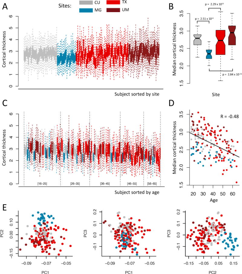
Plots are colored by imaging site: Columbia University (CU), University of Texas Southwestern (TX), Massachusetts General Hospital (MG) and University of Michigan (UM). (a) Boxplots of the cortical thickness sorted by site. Each boxplot represents the distribution of the 98 cortical regions for one subject. (b) Boxplots of the median cortical thickness, grouped by site. The MG site has lower median cortical thickness on average, while the TX and UM sites have higher variability. (c) Same as (a), but sorted by age. Age intervals are included in brackets to help interpretation. (d) Relationship between median cortical thickness and age, colored by site. (e) Plots of the first 3 principal components (PCs) from principal component analysis (PCA), colored by site. The second PC is highly associated with site.

Next, because the scale of the measurements can also be affected by scanner, we also compared the variances of the median cortical thickness measurement across sites. To do so, we performed the Bartlett’s sphericity test [Bartlett, 1937], which assesses whether or not the variances are homogeneous across sites. To avoid confounding of site with age and gender, we first regressed out the variation explained by age and gender; the test was significant (p = 1.8 × 10⁻⁷). We subsequently compared the pairwise site variances using the usual F-tests for variances ratio, and four of the pairs were significant after adjusting for multiple comparisons using Bonferroni correction: TX vs. CU, TX vs. MG, UM vs. CU, and UM vs. MG differed in variance of median cortical thickness.

We also tested each ROI individually for site effects by calculating an ANOVA F-test. We obtained 53 ROIs significantly associated with site, using Bonferroni correction to adjust for multiple comparisons (adjusted p < 0.05). Because Bonferroni correction is a conservative approach to control for the family-wise error rate (FWER), we alternatively corrected for multiple comparisons using the permutation-based one-step maxT procedure [Westfall and Young, 1993, Dudoit et al., 2003], and obtained 60 ROIs significantly associated with site (adjusted p < 0.05, B = 10,000 permutations). We present in Figure A.1a the observed R² from ANOVA and the distribution of the maximum R² obtained from each permutation. To test for scanner-specific scaling effects, we also tested each feature individually for homogeneity of variances across sites using Bartlett’s test. We obtained 41 ROIs with variances significantly associated with site (adjusted p < 0.05, B = 10,000 permutations). The significant regions are reported in Supplementary Table 2.

In Figure 1, we observe a global decrease of the cortical thickness measurements with age, and note that combining measurements from multiple sites adds variability to the trend (blue boxplots are shifted downwards). We also observe that the imaging sites are not distributed equally across the age span, with more younger subjects from the MG and CU sites (more blue and grey boxplots to the left) and older subjects coming from the TX site (more light red boxplots to the right). This indicates some confounding between imaging site and age. In Figure 1d, we present the median cortical thickness measurements as a function of age to visually inspect the global image-age relationship. In Figure 1e, we present bivariate scatter plots of the first 3 principal components (PCs) from a principal component analysis (PCA) performed on the cortical thickness values. We note that the second PC is highly associated with site, confirming that a large proportion of the variation in the data is explained by site.

Finally, we present in Figure 2 the distribution of age, gender, HAMD score and QIDS score across imaging sites. This allows a visual inspection of potential confounding level between the different covariates and imaging site. The width of the boxplots represents the sample size at each site. We note that age is highly imbalanced across sites, with older subjects at the TX site. We also note that gender is imbalanced within each site with a greater number of females. The QIDS score appears to be also imbalanced with respect to imaging site and anti-correlated with age.

Figure 2. Distribution of covariates in the EMBARC study.

Distributions of age, gender, HAMD score and QIDS scores across sites for the EMBARC study. The width of the boxplots is proportional to the number of subjects scanned at each site. The full and shaded bars in the gender barplots represent males and females respectively. HAMD: Hamilton Depression Rating Scale; QIDS: Quick Inventory for Depression Symptomatology. p-values indicate the significant differences in means between the centers. Gender ratios were not significantly different between sites.

VDLC study

In Figure 3b, we present diagnostic plots for the VDLC study. We note in the VDLC study that there is a clear positive shift in the cortical thickness measurements for images acquired on 3T scanners in comparison to images acquired on 1.5T scanners (Figure 3a). Using ANOVA, the median cortical thickness was significantly different across the seven scanners (p = 2.2 × 10⁻¹⁶). Not surprisingly, the median cortical thicknesses from each of the 3T scanners were significantly different from those of each of the 1.5T scanner, adjusting for multiple comparisons using the DLK test. To assess the normality assumption of the t-tests, we first performed the Shapiro-Wilk test for each of the scanners, and the p-values were not significant for most groups in the VDLC study (W_TIMTrio_A: p = 0.07; W_TIMTrio_B: p = 0.42; D_TIMTrio_A: p = 0.004; W_Sonata_A: p = 0.90; W_Sonata_B: p = 0.63; D_TIMTrio_B: p = 0.39; D_SIGNA: p = 0.88). A p-value is significant when the data do not appear to be normal. Only the D_TIMTrio_A scanner appeared to have a non-normal distribution.

Figure 3. Visualization of sites effects in the VDLC study.

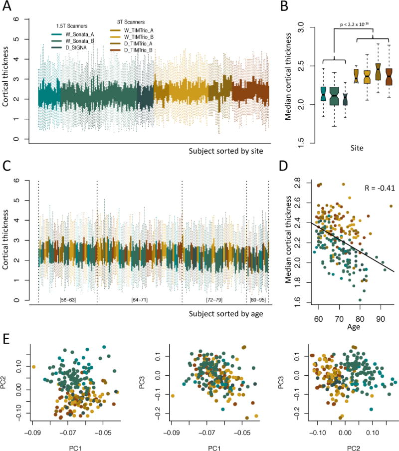
Plots are colored by scanner. The green shades represent the 1.5T scanners, while the brown shades represent the 3T scanners. (a) Boxplots of the cortical thickness sorted by site. Each boxplot represents the distribution of the 98 cortical regions for one subject. (b) Boxplots of the median cortical thickness, grouped by scanner. The measurements derived from 1.5T scanners are substantially lower than measurements from 3T scanners. (c) Same as (a), but sorted by age. Age intervals are included in brackets to help interpretation. (d) Relationship between median cortical thickness and age, colored by scanner. (e) Plots of the first 3 principal components (PCs) from principal component analysis (PCA), colored by scanner. The second PC is highly associated with scanner.

We also compared the variances of the median cortical thickness measurement across scanners. To do so, we performed the Bartlett’s sphericity test, which estimates whether or not the variances are homogeneous across scanners. To avoid confounding of scanner with age and gender, we first regressed out the variation explained by age and gender; the test was significant (p = 0.0013).

We also tested each ROI individually for site effects by calculating an ANOVA F-test. We obtained 86 ROIs significantly associated with site, using Bonferroni correction to adjust for multiple comparisons (adjusted p < 0.05), and 87 ROIs using the permutation-based one step maxT procedure (adjusted p < 0.05, B = 10,000 permutations). We present in Figure A.1b the observed R² from ANOVA and the distribution of the maximum R² obtained from each permutation. To test for scanner-specific scaling effects, we also tested each feature individually for homogeneity of variances across sites using Bartlett’s test. We obtained 4 ROIs with variances significantly associated with site (adjusted p < 0.05, B = 10,000 permutations). The significant regions are reported in Supplementary Table 2.

Finally, we present in Figure 4 the distribution of age, gender, and disease group across scanners. This allows a visual inspection of potential confounding level between the different covariates and imaging site. The width of the boxplots represents the sample size at each site. We note that the average age is significantly different for the D_SIGNA scanner. We also note that the gender ratio is significantly different for the W_Sonata_B scanner, with a significantly larger number of females imaged using this scanner. In the third panel, one can observe that proportions of depressed versus healthy subjects vary greatly across scanners.

Figure 4. Distribution of covariates in the VDLC study.

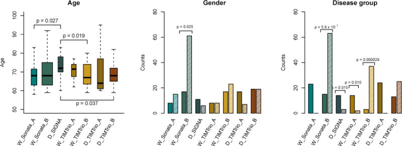
Distributions of age, gender, and disease group for the VDLC study. The width of the boxplots is proportional to the number of subjects scanned at each site. For the age boxplots, the p-values indicate the significant differences in means between sites. The full and shaded bars in the gender barplots represent males and females respectively; the gender ratio was significantly different for the W_Sonata_B scanner. The full and shaded bars in the disease group barplots represent control and depressed subjects respectively. The proportions of subjects with depression were significantly across the 4 scanners.

3.2 Removal of site effects with harmonization

To remove site effects in both the EMBARC and VDLC datasets, we applied three different harmonization techniques: (1) Residuals: removal of site effects estimated from linear regression; (2) Adjusted Residuals: removal of site effects estimated from linear regression, adjusting for biological covariates; and (3) ComBat. We now present the results for both studies separately.

EMBARC Study

In Figure 5, we show the empirical distributions of the site effects for the EMBARC study, for both the location and scale parameters (dotted lines), together with the prior distributions estimated by ComBat (solid lines). We remind the reader that both the location and scale site effects are deviations from the grand mean. Consistent with the description of the site effects in the previous section, we note that the additive site effects (γ) are greater in magnitude for the MG site (Figure 5a, and the multiplicative site effects (δ) are greater than 1 on average for the TX and UM sites and lower than 1 for the two remaining sites (Figure 5b). We note that the prior distributions fit the empirical distributions well for both the location and scale parameters; the ComBat procedure therefore appears appropriate for capturing these effects.

Figure 5. Prior distributions of the site effect parameters estimated by ComBat in the EMBARC study.

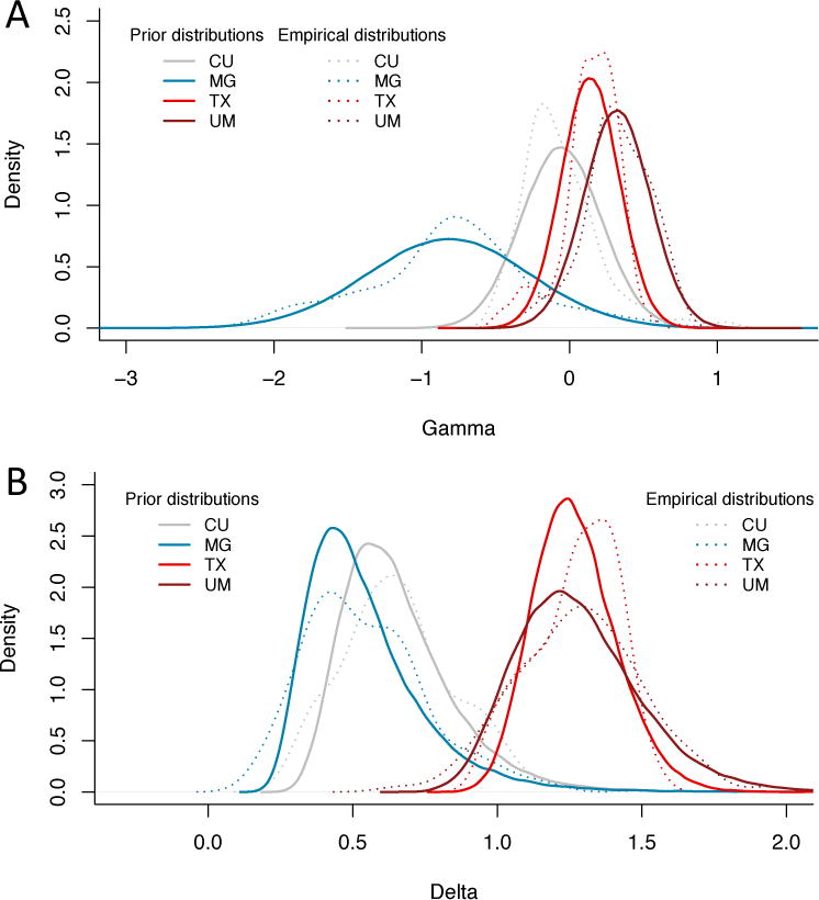
Location and scale site-specific parameters estimated by ComBat, for the EMBARC study. (a) The ComBat-estimated prior distributions for the site-specific location parameters γ are shown in solid lines, and the empirical distributions of the site-specific location parameters are shown in dashed lines. (b) The ComBat-estimated prior distributions for the site-specific scale parameters δ are shown in solid lines, and the empirical distributions of the site-specific scale parameters are shown in dashed lines. The prior distributions fit well the empirical distributions for both the location and scale parameters.

To visualize whether or not most of the variation in the data was still associated with imaging site after harmonization, we first performed an unsupervised dimension reduction of the harmonized cortical thickness measurement using PCA. The data projected into the first two PCs are presented in the first column of Figure 6. We note that for all three harmonization methods, the data points appear to be distributed equally across sites. We also performed a linear discriminant analysis (LDA), a popular supervised dimension reduction that maximizes the projection coordinates to predict the data classes. Here, we use the imaging sites as the data classes to be predicted. We present the projected data in the second column of Figure 6. One can see that for the raw data, the data points cluster almost perfectly by imaging site. This is not surprising; all features are highly associated with site effects when not harmonized. We also note that despite harmonization of the acquisition sequences (for more details on study design, see Trivedi et al. [2016]), the EMBARC study still exhibits inter-site effects before harmonization. Furthermore, note that images acquired on scanners from the same manufacturer tend to cluster together in the LDA plots. After harmonization, site clusters are substantially attenuated.

Figure 6. Supervised and unsupervised dimension reductions before and after harmonization for the EMBARC dataset.

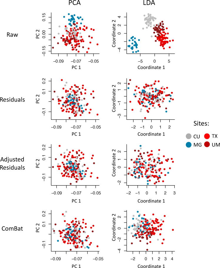
For each harmonization method, we first used principal component analysis (PCA) to reduce the dimension of the cortical thickness measurements in an unsupervised manner (agnostic of imaging sites). We present in the first column the projection of the data into the first two principal components (PCs) that explain most of the variation in the data. We also performed a supervised dimension reduction technique using linear discriminant analysis (LDA) using imaging site as a target variable. We present in the second column the projection of the data into the first two LDA coordinates. In both PCA and LCA, the first two coordinates are highly associated with site, while all harmonization methods removed most variation associated with site.

To formally test whether or not site effects remain after harmonization, we again used the different tests described in Section 3.1. Using ANOVA F-tests, all methods corrected for mean site differences in the median cortical thickness: p = 0.997 for Residuals, p = 0.0498 for Adjusted Residuals and p = 0.0473 for ComBat. We also tested for site-specific scaling effect in the measurements using Bartlett’s sphericity test. We found that only ComBat was able to remove the scaling effects associated with site (p = 0.42). The site-specific variances remained largely uncorrected for both the Residuals (p = 2.53 × 10⁻⁸) and Adjusted Residuals (p = 3.08 × 10⁻⁸) methods. This is not surprising; only the ComBat harmonization method is able to model scaling factors associated with site. We also tested each ROI individually for remaining site effects. For all harmonization methods, none of the ROIs was significantly associated with site, using either the Bonferroni or the maxT adjustment.

Finally, to further investigate if site effects were entirely removed for each of the harmonization method, we attempted to predict imaging site from the harmonized cortical thickness features. More specifically, we used the support vector machine (SVM) [Cortes and Vapnik, 1995] classification algorithm, with radial basis kernel, to predict site from the imaging features. The SVM is largely used in the imaging community in the context of multivariate pattern analysis (MPVA) for understanding and discovering patterns associated with a disease outcome, for instance. A harmonization method that is successful in removing site effects will result in a lower SVM accuracy when attempting to predict site. Using B = 10,000 repetitions of a 10-fold cross-validation, we estimated an average accuracy for each method. For the raw values, the SVM prediction achieved an average of 76.6% classification accuracy. For the residuals and adjusted residuals methods, the average accuracies were 40.5% and 38.7% respectively. The ComBat method resulted in the lower average accuracy (36.3%). Using a permutation-based approach to generate a null distribution (B = 10, 000), a SVM classification by chance attained on average 36.9% accuracy. This indicates the Adjusted Residuals and ComBat were best for the removal of site effects in the cortical thickness measurements. In comparison to the adjusted residuals, we note that the ComBat method additionally removes site-specific scaling effects. This could explain the better performance in the SVM, in which the covariance structure is implicitly used for predicting the class labels.

VDLC study

In Figure 7, we show the empirical distributions of the site effects for the VDLC study, for both the location and scale parameters (dotted lines), together with the prior distributions estimated by ComBat (solid lines). Consistent with the description of the site effects in the previous section, we note that the additive scanner effects (γ) are greater in magnitude for the 3T scanners. The multiplicative scanner effects (δ) are shown in Figure 7b. We note that the prior distributions fit the empirical distributions well for both the location and scale parameters; the ComBat procedure therefore appears appropriate for capturing these effects.

Figure 7. Prior distributions of the site effect parameters estimated by ComBat in the VDLC study.

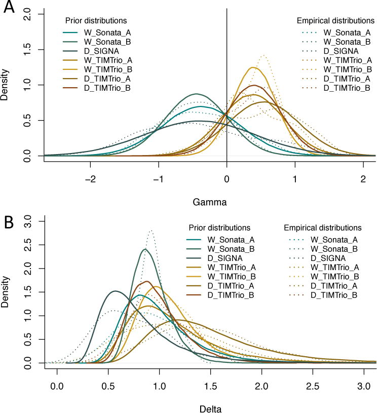
Location and scale site-specific parameters estimated by ComBat, for the VDLC study. (a) The ComBat-estimated prior distributions for the site-specific location parameters γ are shown in solid lines, and the empirical distributions of the site-specific location parameters are shown in dashed lines. (b) The ComBat-estimated prior distributions for the site-specific scale parameters δ are shown in solid lines, and the empirical distributions of the site-specific scale parameters are shown in dashed lines. The prior distributions fit well the empirical distributions for both the location and scale parameters.

To visualize whether or not most of the variation in the data was still associated with scanner after harmonization, we first performed an unsupervised dimension reduction of the harmonized cortical thickness measurement using PCA. The data projected into the first two PCs are presented in the first column of Figure 8. We note that for all three harmonization methods, the data points appear to be distributed equally across scanners. We also performed LDA using scanners as the data classes. We present the projected data in the second column of Figure 8. One can see that for the raw data, there is a clear separation between the different types of scanners. Interestingly, the data from the D SIGNA scanner appear to cluster separately; we note that this is the only GE scanner in the VDLC study. After harmonization, clusters associated with scanner are substantially attenuated.

Figure 8. Supervised and unsupervised dimension reductions before and after harmonization for the VDLC dataset.

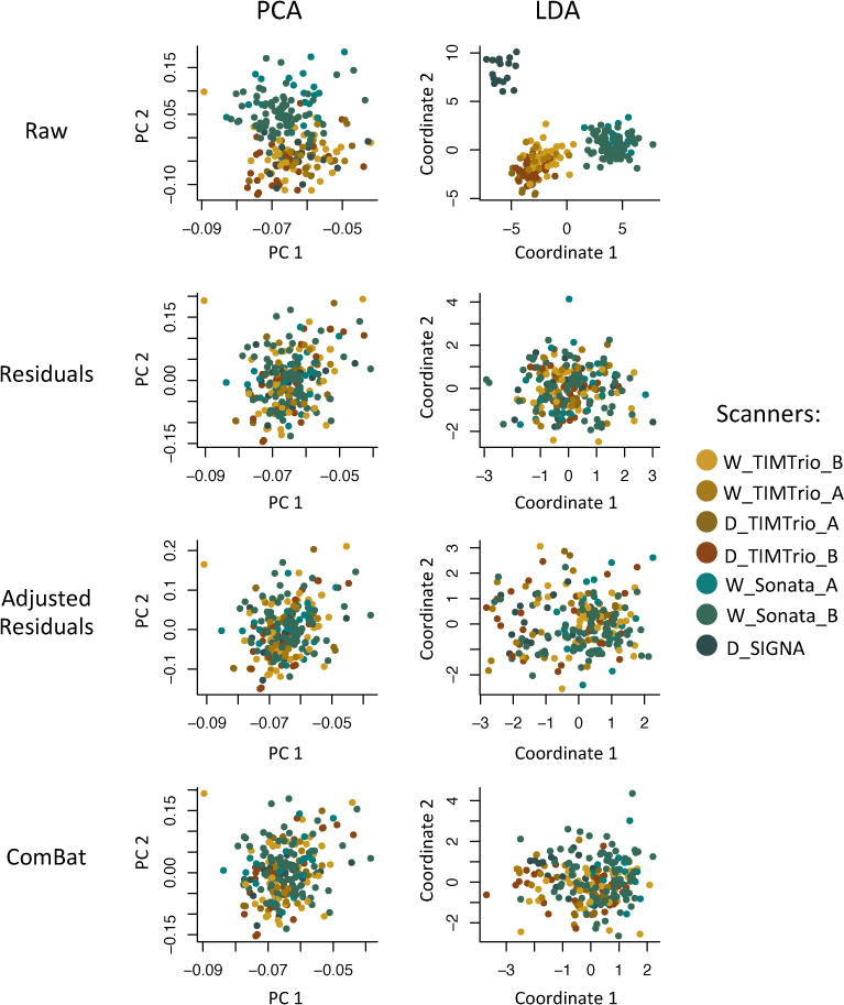
For each harmonization method, we first used principal component analysis (PCA) to reduce the dimension of the cortical thickness measurements in an unsupervised manner (agnostic of imaging sites). We present in the first column the projection of the data into the first two principal components (PCs) that explain most of the variation in the data. We also performed a supervised dimension reduction technique using linear discriminant analysis (LDA) using imaging site as a target variable. We present in the second column the projection of the data into the first two LDA coordinates. In both PCA and LCA, the first two coordinates are highly associated with site, while all harmonization methods removed most variation associated with site.

Using ANOVA F-tests, all methods corrected for mean scanner differences in the median cortical thickness: p = 0.99 for Residuals, p = 0.94 for Adjusted Residuals and p = 0.94 for ComBat. We also tested for scanner-specific scaling effects in the measurements using Bartlett’s sphericity test. We found that only ComBat was able to remove the scaling effects associated with scanner (p = 0.46). Scanner-specific variances remained present in both the Residuals (p = 0.03) and Adjusted Residuals (p = 0.01) methods. Finally, we tested each ROI individually for remaining scanner effects. For all harmonization methods, none of the ROIs was significantly associated with scanner, using either the Bonferroni or the maxT adjustment.

As conducted in the EMBARC study, we used the SVM with radial basis kernel to assess prediction of scanner from the imaging features. Again, a harmonization method that is successful in removing scanner effects will result in a lower SVM accuracy when attempting to predict scanner. Using B = 10,000 repetitions of a 10-fold cross-validation, we estimated an average accuracy for each method. For the raw values, the SVM prediction achieved an average of 67.7% classification accuracy. For the residuals and adjusted residuals methods, the average accuracies were 43.4% and 44.4% respectively. The ComBat method resulted in the lowest average accuracy (41.0%).

3.3 Associations with age

While it is important to show that a harmonization method successfully removes site effects, it is equally important to show that the method preserves the biological variability in the data; a method that removes both site effects and biological effects has no scientific use. To investigate whether or not the different harmonizations presented in this paper perform well at preserving biological variability, we use age as a variable of interest.

We assessed the proportion of variation explained by age before and after harmonization. Without harmonization, the percentage of variation in the average cortical thickness explained by age was 23%. This was calculated using the usual coefficient of variation R² from linear regression with median cortical thickness as the outcome. For the unadjusted Residuals method, this percentage was increased to 26%, and for both the Adjusted Residuals and ComBat, the percentage was increased to 33%. The fact that the Unadjusted Residuals did not substantially increase the association with age is not surprising; we observed that age was confounded with imaging site, and therefore removing site effects without adjusting for age will also remove variation in the imaging features associated with age. On the other hand, both the Adjusted Residuals and ComBat strengthened the expected inverse relationship between age and cortical thickness by removing site effects, but also by preserving biological variability in the data.

We also evaluated the effects of harmonization on the prediction of age using the harmonized cortical thickness measurements. For prediction, we used two different algorithms: linear regression, and the popular support vector regression (SVR) algorithm, also commonly called ε-SVM regression, using two different kernels: a linear kernel and a radial basis function. The ε-SVM regression paradigm is similar to the regular classification SVM, but for a continuous outcome. For each algorithm, we used the cortical thickness measurements of the 98 cortical regions as imaging features inputs to predict age (98 values per participant). For each harmonization method, we randomly partitioned the subjects into k folds, and trained the prediction algorithm on k −1 folds. We then predicted the age of the remaining subjects (testing dataset) and calculated the root-mean-square error (RMSE). We repeated the random sampling B = 1000 times, for k ∈ {3, 5, 10}, to obtain a distribution of the RMSE for each method at each k. For each random sampling, we selected the hyperparameters that led to the best cross-validated performance by performing a grid search with the following grid values: C ∈ {0.001, 0.1, 1, 10, 100, 1000} and ε ∈ {0.01, 0.1, 0.5, 1}.

In Figure 9, we present the results from linear regression. For the three values of k, we observe that the data harmonized with the unadjusted Residuals do not perform well (substantial increase of RMSE). On the other hand, both the Adjusted Residuals and ComBat significantly improve the average prediction accuracy compared with the raw data (p < 0.05 for all k). In Figure 10, we present the results from ε-SVM regression using a linear kernel. For the three values of k, the Adjusted residuals improve the age prediction compared to the raw data; Combat performs either equally (k = 3, 10), or improves the performance (k = 5). As it is the case for Figure 9, the unadjusted Residuals worsens the age prediction. In Figure 11, we present the results from ε-SVM regression using a radial basis function kernel. While the Adjusted Residuals and ComBat perform similarly to the raw data for the three values of k (no significant difference in the RMSE), the unadjusted Residuals substantially increases the RMSE.

Figure 9. Root-mean-square error (RMSE) for age prediction using linear regression.

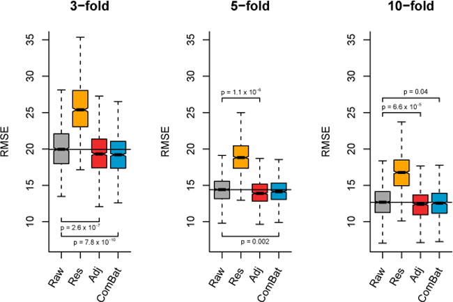
Using k-fold validation for k ∈ {3, 5, 10} for B = 1000 random samplings, we calculated the RMSE on a testing dataset for the predicted age using linear regression. For the different harmonization methods, we used the harmonized cortical thickness measurements as input image features to train the algorithm. The p-values represent significant reductions of RMSE with respect to the raw data.

Figure 10. Root-mean-square error (RMSE) for age prediction using ε-SVM (linear kernel).

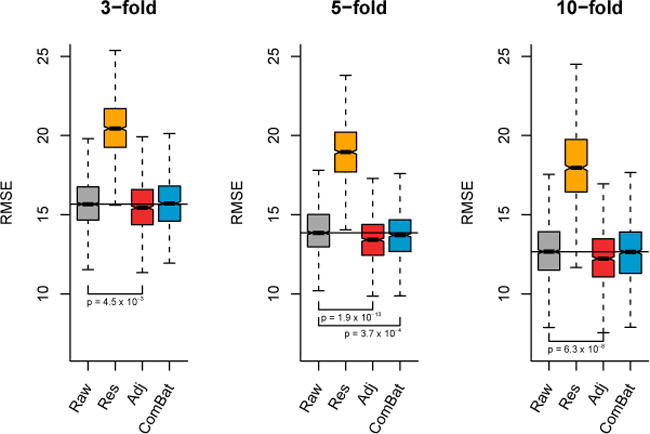
Using k-fold validation for k ∈ {3, 5, 10} for B = 1000 random samplings, we calculated the RMSE on a testing dataset for the predicted age using ε-SVM with a linear kernel. For the different harmonization methods, we used the harmonized cortical thickness measurements as input image features to train the algorithm.

Figure 11. Root-mean-square error (RMSE) for age prediction using ε-SVM (radial basis function kernel).

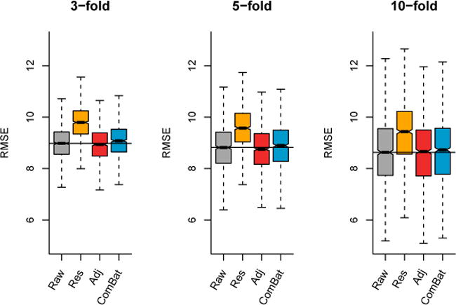
Using k-fold validation for k ∈ {3, 5, 10} for B = 1000 random samplings, we calculated the RMSE on a testing dataset for the predicted age using ε-SVM with a radial basis function kernel. For the different harmonization methods, we used the harmonized cortical thickness measurements as input image features to train the algorithm.

Overall, the removal of unwanted site effects with both ComBat and the Adjusted Residuals did not decrease our ability to predict age, either using linear regression or SVMs. This confirms that both methods preserved biological variability associated with age, a crucial requirement for adequate multi-site harmonization. On the other hand, the unadjusted Residuals substantially decreased the predictive performance. This shows that failing to account for age when removing site effects in an unbalanced sample leads to removal of age-related signal, as described in Rao et al. [2017].

3.4 Life-span study by harmonizing the EMBARC and VDLC datasets

While the two studies present in this paper have a different age range ([18,65] y.o. for the EMBARC study; [58,95] y.o. for the VDLC study), there is some overlap between the two age ranges (see Figure 12, first panel). For the study of life-span trajectories, it is sometimes necessary to combine data from multiple studies, with each individual study often targeting participants from a specific age range. We show here that even though different scanners and slightly different cortical thickness ROI extraction methods were used across the studies, it is possible to combine and harmonize the data, to remove the scanner effects, and thereby improve the correlation between the imaging outcome and biological factors of interest, namely age.

Figure 12. Median age trajectory before and after harmonization.

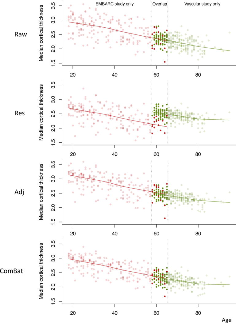
The EMBARC and VDLC studies were combined using different harmonizations. The red dots represent the median cortical thickness for the EMBARC study participants, and the greens dots represent the median cortical thickness for the VDLC study participants. The curves represent the lowess fitted values for each study separately.

We present the relationship between median cortical thickness and age, before and after harmonization in Figure 12 with data points colored by study (red for EMBARC and green for VDLC). One can observe an overlap in the age span between the two studies, and that inter-subject variation seems to be higher in the EMBARC subjects in the raw data. This can be explained by the large variation between the four scanners in the EMBARC, as discussed previously in the Results section. For each method, we calculated the correlation between the median cortical thickness and age. For the unharmonized data, we obtained a correlation of − 0.70. For the unadjusted Residuals, we obtained a correlation of −0.26. Such a weaker correlation is not surprising; both studies have a vastly different age range, and therefore blindly harmonizing the data for site without adjusting by age will diminish the age effect across the life span. For the Adjusted Residuals, we obtained a correlation of −0.77, and we obtained a correlation of −0.79 for ComBat. Both adjusted residualization and ComBat were effective at decreasing the inter-subject variability by removing scanner effects, while preserving the trend associated with age across the life-span.

3.5 Associations with gender

We also investigated the impact of harmonizing the EMBARC and VDLC studies together on the associations between cortical thickness measurements and gender. Before harmonization (raw data), 30 cortical regions were significantly associated with gender, after adjusting for multiple comparisons using the Benjamini-Hochberg procedure (p < 0.05). Interestingly, after harmonizing the data using either the unadjusted Residuals, the Adjusted Residuals, or the ComBat approach, we found that none of the features were associated with gender.

To investigate whether or not the results from the raw data consisted of false positives as a consequence of gender ratios that are imbalanced across sites (see Figure 4), we devised the following subsampling strategy: to obtain unconfounded assessments of the associations of gender with cortical thickness measurements, we sampled an equal number of females and males from each scanner at random, resulting in a total of n = 306 subjects; we repeated the random subsampling B = 1000 times. While the resulting total sample size of the matched datasets is smaller, the gender associations in the matched datasets should not be confounded by unwanted scanner variation, and therefore lead to results that are more reflective of the truth. For each of the B = 1000 matched datasets, we calculated the number of features associated with gender, again adjusting for multiple comparisons using the Benjamini-Hochberg procedure. We obtained that more than 98% of the time (981 datasets), there was 0 feature associated with gender, confirming that the 30 features associated with gender in the original raw data are most likely false positives.

In light of these results, it appears that the three harmonization techniques are effective at reducing the number of false positives. Such false positives are most likely features that are artificially associated with a biological covariate of interest, as a result of the biological covariate being unbalanced across scanners or sites.

4 Discussion

With the increasing complexity of study design in multi-site neuroimaging studies, the neuroscience community needs robust, validated, and computationally feasible methods for addressing the critical impact of non-biological sources of data variation. We use the term “harmonization” to refer to the process of combining data from multiple sites and removing the unwanted variability associated with scanner.

In this paper, we proposed to use the ComBat algorithm, previously developed to deal with batch effects in the study of gene expression data, as a reliable harmonization method for combining cortical thickness measurements across sites. This was motivated by its previously documented excellent performance for harmonizing voxel-wise fractional anisotropy (FA) and mean diffusivity (MD) measurements [Fortin et al., 2017], two common DTI scalar maps. Using two large multi-site studies, EMBARC and VDLC, we presented a general approach for identifying unwanted sources of variance in neuroimaging data. We then showed that ComBat is effective at removing nuisance variability associated with scanners, while preserving the age effects in the cortical thickness across participants. We also showed that ComBat can be used to combine those two large studies, with a vastly different age range, to study cortical thickness across the life span. Indeed, while the extraction of thickness in the ROIs was slightly different for the two studies, we nonetheless found ComBat to effectively mitigate scanner effects. We expect future studies of ComBat for addressing minor differences in image processing across studies to evaluate the feasibility of distributed analyses in which only post-processed data are available.

While our analyses of harmonized data did not yield any differences between males and females in cortical thickness measures, there is a significant literature documenting these differences [Luders et al., 2006, Sowell et al., 2006, Gennatas et al., 2017]. These studies used different analytic pipelines to calculate cortical thickness, although we would expect our ANTsCT pipeline to provide similar results. However, previously reported results were based were conducted in healthy individuals, and several were specifically designed to study sex differences, in contrast to the VLDC and EMBARC studies which included large numbers of depressed subjects and were heterogeneous in their demographics across sexes. We expect that future analyses of sex effects from multi-center studies of normal subjects using ComBat to replicate the well-established differences in thickness measures.

We note that ComBat performs well for removing systematic biases associated with scanner in studies independently of whether acquisition protocols were carefully harmonized. In the EMBARC study, for example, inter-site effects were present despite such harmonization; similar differences have recently been reported in volumetric measurements from another multi-center study which used a traveling subject design [Shinohara et al., 2017]. As we found that ComBat was effective in removing effects associated with differences in acquisition protocol and scanner as in the VDLC study, as well as residual site effects from images acquired using the harmonized protocol in the EMBARC.

We compared the ComBat harmonization algorithm to two commonly-used scanner effect correction methods: residualization and adjusted residualization. The latter method adjusts for covariates of interest (for instance age) in the removal of site effects. ComBat is similar to the adjusted method, except that it additionally models scanner-specific scaling effects. ComBat also uses a Bayesian framework to improve the stability of the estimated parameters in small sample sizes. ComBat is easy to apply and has minimal computational overhead. Equally importantly, we have developed open-source, easy-to-use code for applying this algorithm in R, Matlab, and Python. This ensures that the ComBat algorithm can be seamlessly integrated into any existing processing pipelines.

Another advantage of ComBat is its ability to scale up for large neuroimaging studies. Indeed, the ComBat algorithm scales linearly with the number of imaging features, which makes the procedure suitable to image analyses performed at the voxel level, where the number of voxels can often be in the millions. We note that for brainwide analyses performed at the voxel level, the assumptions of the ComBat methodology that scanner effects are shared across all voxels might not be valid. In previous work, our group and others have found that scanner effects on image intensities can be dependent on tissue class, and thus adjustments for site effects may necessitate tissue class-specific modeling. One possible solution is to apply ComBat on each tissue separately. An alternative would be to extend the ComBat model to allow for a mixture of empirical distributions for the scanner effects.

We note that several other harmonization techniques have been previously proposed in the context of other imaging modalities. For instance, for conventional MRI studies, intensity normalization techniques have been developed to make the image intensities comparable across studies, including histogram matching [Nyúl et al., 2000], WhiteStripe [Shinohara et al., 2014] and RAVEL [Fortin et al., 2016]. Another method, called source-based morphometry, uses independent component analysis (ICA) to remove variability associated with certain scanner parameters in structural MRI [Chen et al., 2014]. For diffusion tensor imaging (DTI) studies, it has been proposed to use spherical harmonics to harmonize data across studies, using a reference site to create pairwise site transformations [Mirzaalian et al., 2016]. It has also been proposed to use functional normalization, originally developed in [Fortin et al., 2014], for harmonizing DTI scalar maps.

The aforementioned harmonization techniques cannot be readily applied to cortical thickness. For instance, for WhiteStripe and RAVEL, control features in the WM and in the CSF are required, which do not make sense in the context of cortical thickness measurements in the GM. Furthermore, the histogram matching method attempts to estimate the histogram peaks for each of the GM, WM and CSF tissues, and then aligns these peaks across images to make the intensities comparable. Again, this technique is not applicable to cortical thickness measurements in the GM. On the other hand, ComBat does not make such specific assumptions on the nature of the imaging measurements, making it a potential and versatile tool for the harmonization of multi-site imaging studies for other modalities.

In the future, we plan to develop a time-dependent ComBat algorithm for understanding scenarios where subjects were scanned over multiple time points, and for which scans were acquired on different scanners, or on the same scanners but with different scanning parameters. We are also planning on improving the performance of ComBat in the presence of confounding by implementing an inverse probability weighting (IPW) scheme into the algorithm. IPW has been shown to improve prediction when the outcome of interest is confounded with another covariate [Linn et al., 2016]. This has the potential to improve the performance of ComBat for age prediction using the SVM regression framework, as well as for other prediction methods.

5 Software

All postprocessing analysis was performed in the R statistical software (version 3.2.0). For ComBat, the reference implementations from the sva package was used. All figures were generated in R with customized and reproducible scripts. We have adapted and implemented the ComBat methodology to imaging data, and the software is available in R and Matlab (https://github.com/Jfortin1/ComBatHarmonization ) and in Python (https://github.com/ncullen93/neuroCombat).

Table 1.

Description of the EMBARC and VDLC study samples

Scanner	N subjects	N females (%)	Age range	N Depressed (%)
EMBARC study	187	116 (62)	[18,65]	187 (100)
CU	46	29 (63)	[18,61]	46 (100)
MG	26	21 (81)	[18,60]	26 (100)
TX	72	42 (58)	[19,65]	72 (100)
UM	43	24 (56)	[18,59]	43 (100)
VDLC study	236	139 (59)	[58,95]	177 (75)
W_Sonata_A	23	15 (65)	[58,83]	23 (100)
W_Sonata_B	78	61 (78)	[59,92]	62 (81)
W_TIMTrio_A	16	8 (50)	[62,85]	2 (13)
W_TIMTrio_B	40	23 (58)	[59,80]	37 (93)
D_TIMTrio_A	24	7 (29)	[60,95]	24 (100)
D_TIMTrio_B	38	19 (50)	[59,84]	25 (66)
D_SIGNA	17	6 (35)	[60,83]	3 (18)

Abbreviations

ANTs

Advanced normalization tools

AD

Alzheimer’s disease

ADNI

Alzheimer’s Disease Neuroimaging Initiative

ANOVA

Analysis of variance

CSF

Cerebrospinal Fluid

DiReCT

Diffeomorphic Registration Based Cortical Thickness

DTI

Diffusion tensor imaging

EB

Empirical Bayes

EMBARC

Establishing Moderators and Biosignatures of Antidepressant Response in Clinical care

FA

Fractional anisotropy

FWER

Family-wise error rate

GM

Grey Matter

GPR

Gaussian process regression

HAMD

Hamilton Depression Rating Scale

IPW

Inverse probability weighting

LDA

Linear discriminant analysis

LLD

Late-life depression

MALF

Multi-atlas label fusion

MASQ

Mood and Anxiety Symptom Questionnaire

MCI

Mild cognitive impairment

MD

Mean diffusivity

MVPA

Multivariate pattern analysis

OASIS

Open Access Series of Imaging Studies

PC

Principal component

PCA

Principal component analysis

QIDS

Quick Inventory for Depression Symptomatology

RMSE

Root-mean-square error

ROI

Region of interest

STAI

Spielberger State-Trait Anxiety Inventory

SVM

Support vector machine

SVR

Support vector regression

VDLC

Vascular disease: Longitudinal changes

WM

White Matter

Appendix A

Figure A.1. Variance explained by imaging site (R²).

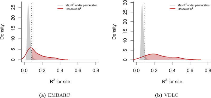
For each feature, we calculated the coefficient of determination R² between cortical thickness and imaging site. We present the densities of R² (red lines) for the (a) EMBARC study and the (b) VDLC study. To obtain a measure of significance and to correct for multiple comparisons, we performed a one-step max R² procedure. Briefly, we permuted the site labels B = 10, 000 times, recalculated the R² values and retained the maximum R² value at each permeation. The grey densities represent the distribution of the maximum R²’s. The vertical dashed line indicates the 95% quantile of the maximum R² distribution. The features above that threshold are significant at the α = 0.05 level (shaded red area). Most features remained significant after adjustment.

References

- Avants Brian B, Tustison Nicholas J, Wu Jue, Cook Philip A, Gee James C. An open source multivariate framework for n-tissue segmentation with evaluation on public data. Neuroinformatics. 2011;9(4):381–400. doi: 10.1007/s12021-011-9109-y. [DOI] [PMC free article] [PubMed] [Google Scholar]
- Barch Deanna M, D’Angelo Gina, Pieper Carl, Wilkins Consuelo H, Welsh-Bohmer Kathleen, Taylor Warren, Garcia Keith S, Gersing Kenneth, Doraiswamy P Murali, Sheline Yvette I. Cognitive improvement following treatment in late-life depression: relationship to vascular risk and age of onset. The American Journal of Geriatric Psychiatry. 2012;20(8):682–690. doi: 10.1097/JGP.0b013e318246b6cb. [DOI] [PMC free article] [PubMed] [Google Scholar]
- Bartlett Maurice S. Properties of sufficiency and statistical tests. Proceedings of the Royal Society of London. Series A, Mathematical and Physical Sciences. 1937:268–282. [Google Scholar]
- Jiayu Chen Jingyu Liu, Calhoun Vince D, Arias-Vasquez Alejandro, Zwiers Marcel P, Gupta Cota Navin, Franke Barbara, Turner Jessica A. Exploration of scanning effects in multi-site structural mri studies. Journal of neuroscience methods. 2014;230:37–50. doi: 10.1016/j.jneumeth.2014.04.023. [DOI] [PMC free article] [PubMed] [Google Scholar]
- Cortes Corinna, Vapnik Vladimir. Support-vector networks. Machine learning. 1995;20(3):273–297. [Google Scholar]
- Das Sandhitsu R, Avants Brian B, Grossman Murray, Gee James C. Registration based cortical thickness measurement. Neuroimage. 2009;45(3):867–879. doi: 10.1016/j.neuroimage.2008.12.016. [DOI] [PMC free article] [PubMed] [Google Scholar]
- Martino Adriana Di, Yan Chao-Gan, Li Qingyang, Denio Erin, Castellanos Francisco X, Alaerts Kaat, Anderson Jeffrey S, Assaf Michal, Bookheimer Susan Y, Dapretto Mirella, et al. The autism brain imaging data exchange: towards a large-scale evaluation of the intrinsic brain architecture in autism. Molecular psychiatry. 2014;19(6):659–667. doi: 10.1038/mp.2013.78. [DOI] [PMC free article] [PubMed] [Google Scholar]
- Dudoit Sandrine, Shaffer Juliet Popper, Boldrick Jennifer C. Multiple hypothesis testing in microarray experiments. Statistical Science. 2003:71–103. [Google Scholar]
- Dunnett Charles W. Pairwise multiple comparisons in the unequal variance case. Journal of the American Statistical Association. 1980;75(372):796–800. [Google Scholar]
- Fortin Jean-Philippe, Labbe Aurelie, Lemire Mathieu, Zanke Brent, Hudson Thomas, Fertig Elana, Greenwood Celia, Hansen Kasper D. Functional normalization of 450k methylation array data improves replication in large cancer studies. Genome Biology. 2014;15(11):503. doi: 10.1186/s13059-014-0503-2. [DOI] [PMC free article] [PubMed] [Google Scholar]
- Jean-Philippe Fortin Elizabeth M Sweeney, Muschelli John, Crainiceanu Ciprian M, Shinohara Russell T, Alzheimer’s Disease Neuroimaging Initiative et al. Removing inter-subject technical variability in magnetic resonance imaging studies. NeuroImage. 2016;132:198–212. doi: 10.1016/j.neuroimage.2016.02.036. [DOI] [PMC free article] [PubMed] [Google Scholar]
- Fortin Jean-Philippe, Parker Drew, Tunc Birkan, Watanabe Takanori, Elliott Mark A, Ruparel Kosha, Roalf David R, Satterthwaite Theodore D, Gur Ruben C, Gur Raquel E, Schultz Robert T, Verma Ragini, Shinohara Russell T. Harmonization of multi-site diffusion tensor imaging data. bioRxiv. 2017 doi: 10.1101/116541. URL http://biorxiv.org/content/early/2017/03/15/116541. [DOI] [PMC free article] [PubMed]
- Gennatas Efstathios D, Avants Brian B, Wolf Daniel H, Satterthwaite Theodore D, Ruparel Kosha, Ciric Rastko, Hakonarson Hakon, Gur Raquel E, Gur Ruben C. Age-related effects and sex differences in gray matter density, volume, mass, and cortical thickness from childhood to young adulthood. Journal of Neuroscience. 2017;37(20):5065–5073. doi: 10.1523/JNEUROSCI.3550-16.2017. [DOI] [PMC free article] [PubMed] [Google Scholar]
- Greenberg Tsafrir, Chase Henry W, Almeida Jorge R, Stiffler Richelle, Zevallos Carlos R, Aslam Haris A, Deckersbach Thilo, Weyandt Sarah, Cooper Crystal, Toups Marisa, et al. Moderation of the relationship between reward expectancy and prediction error-related ventral striatal reactivity by anhedonia in unmedicated major depressive disorder: findings from the embarc study. American Journal of Psychiatry. 2015;172(9):881–891. doi: 10.1176/appi.ajp.2015.14050594. [DOI] [PMC free article] [PubMed] [Google Scholar]
- Hamilton Max. A rating scale for depression. Journal of Neurology, Neurosurgery & Psychiatry. 1960;23(1):56–62. doi: 10.1136/jnnp.23.1.56. [DOI] [PMC free article] [PubMed] [Google Scholar]
- Han Xiao, Jovicich Jorge, Salat David, van der Kouwe Andre, Quinn Brian, Czanner Silvester, Busa Evelina, Pacheco Jenni, Albert Marilyn, Killiany Ronald, et al. Reliability of mri-derived measurements of human cerebral cortical thickness: the effects of field strength, scanner upgrade and manufacturer. Neuroimage. 2006;32(1):180–194. doi: 10.1016/j.neuroimage.2006.02.051. [DOI] [PubMed] [Google Scholar]
- Johnson W Evan, Li Cheng, Rabinovic Ariel. Adjusting batch effects in microarray expression data using empirical bayes methods. Biostatistics. 2007;8(1):118–127. doi: 10.1093/biostatistics/kxj037. [DOI] [PubMed] [Google Scholar]
- Jovicich Jorge, Czanner Silvester, Greve Douglas, Haley Elizabeth, Kouwe Andre van der, Gollub Randy, Kennedy David, Schmitt Franz, Brown Gregory, MacFall James, et al. Reliability in multi-site structural mri studies: effects of gradient non-linearity correction on phantom and human data. Neuroimage. 2006;30(2):436–443. doi: 10.1016/j.neuroimage.2005.09.046. [DOI] [PubMed] [Google Scholar]
- Keator David B, Helmer K, Steffener Jason, Turner Jessica A, Van Erp Theo GM, Gadde Syam, Ashish Naveen, Burns GA, Nichols B Nolan. Towards structured sharing of raw and derived neuroimaging data across existing resources. Neuroimage. 2013;82:647–661. doi: 10.1016/j.neuroimage.2013.05.094. [DOI] [PMC free article] [PubMed] [Google Scholar]
- Klein Arno, Andersson Jesper, Ardekani Babak A, Ashburner John, Avants Brian, Chiang Ming-Chang, Christensen Gary E, Collins D Louis, Gee James, Hellier Pierre, et al. Evaluation of 14 nonlinear deformation algorithms applied to human brain mri registration. Neuroimage. 2009;46(3):786–802. doi: 10.1016/j.neuroimage.2008.12.037. [DOI] [PMC free article] [PubMed] [Google Scholar]
- Leek Jeffrey T, Scharpf Robert B, Bravo Héctor Corrada, Simcha David, Langmead Benjamin, Johnson W Evan, Geman Donald, Baggerly Keith, Irizarry Rafael A. Tackling the widespread and critical impact of batch effects in high-throughput data. Nature Reviews Genetics. 2010;11(10):733–739. doi: 10.1038/nrg2825. [DOI] [PMC free article] [PubMed] [Google Scholar]
- Linn Kristin A, Gaonkar Bilwaj, Doshi Jimit, Davatzikos Christos, Shinohara Russell T. Addressing confounding in predictive models with an application to neuroimaging. The international journal of biostatistics. 2016;12(1):31–44. doi: 10.1515/ijb-2015-0030. [DOI] [PMC free article] [PubMed] [Google Scholar]
- Luders Eileen, Narr Katherine L, Thompson Paul M, Rex David E, Woods Roger P, DeLuca Heather, Jancke Lutz, Toga Arthur W. Gender effects on cortical thickness and the influence of scaling. Human brain mapping. 2006;27(4):314–324. doi: 10.1002/hbm.20187. [DOI] [PMC free article] [PubMed] [Google Scholar]
- Marcus Daniel S, Wang Tracy H, Parker Jamie, Csernansky John G, Morris John C, Buckner Randy L. Open access series of imaging studies (oasis): cross-sectional mri data in young, middle aged, nondemented, and demented older adults. Journal of cognitive neuroscience. 2007;19(9):1498–1507. doi: 10.1162/jocn.2007.19.9.1498. [DOI] [PubMed] [Google Scholar]
- Mennes Maarten, Biswal Bharat B, Castellanos F Xavier, Milham Michael P. Making data sharing work: the fcp/indi experience. Neuroimage. 2013;82:683–691. doi: 10.1016/j.neuroimage.2012.10.064. [DOI] [PMC free article] [PubMed] [Google Scholar]
- Mettenburg Joseph M, Benzinger Tammie L, Shimony Joshua S, Snyder Abraham Z, Sheline Yvette I. Diminished performance on neuropsychological testing in late life depression is correlated with microstructural white matter abnormalities. Neuroimage. 2012;60(4):2182–2190. doi: 10.1016/j.neuroimage.2012.02.044. [DOI] [PMC free article] [PubMed] [Google Scholar]
- Mirzaalian H, Ning L, Savadjiev P, Pasternak O, Bouix S, Michailovich O, Grant G, Marx CE, Morey RA, Flashman LA, et al. Inter-site and inter-scanner diffusion mri data harmonization. NeuroImage. 2016;135:311–323. doi: 10.1016/j.neuroimage.2016.04.041. [DOI] [PMC free article] [PubMed] [Google Scholar]
- Nyúl LG, Udupa JK, Zhang X. New variants of a method of mri scale standardization. IEEE Trans Med Imaging. 2000 Feb;19(2):143–50. doi: 10.1109/42.836373. [DOI] [PubMed] [Google Scholar]
- Rao Anil, Monteiro Joao M, Mourao-Miranda Janaina, Alzheimer’s Disease Initiative et al. Predictive modelling using neuroimaging data in the presence of confounds. NeuroImage. 2017 doi: 10.1016/j.neuroimage.2017.01.066. [DOI] [PMC free article] [PubMed] [Google Scholar]
- John Rush A, Trivedi Madhukar H, Ibrahim Hicham M, Carmody Thomas J, Arnow Bruce, Klein Daniel N, Markowitz John C, Ninan Philip T, Kornstein Susan, Manber Rachel, et al. The 16-item quick inventory of depressive symptomatology (qids), clinician rating (qids-c), and self-report (qids-sr): a psychometric evaluation in patients with chronic major depression. Biological psychiatry. 2003;54(5):573–583. doi: 10.1016/s0006-3223(02)01866-8. [DOI] [PubMed] [Google Scholar]
- Shinohara RT, Oh J, Nair G, Calabresi PA, Davatzikos C, Doshi J, Henry RG, Kim G, Linn KA, Papinutto N, et al. Volumetric analysis from a harmonized multisite brain mri study of a single subject with multiple sclerosis. American Journal of Neuroradiology. 2017 doi: 10.3174/ajnr.A5254. [DOI] [PMC free article] [PubMed] [Google Scholar]
- Shinohara Russell T, Sweeney Elizabeth M, Goldsmith Jeff, Shiee Navid, Mateen Farrah J, Calabresi Peter A, Jarso Samson, Pham Dzung L, Reich Daniel S, Crainiceanu Ciprian M, Australian Imaging Biomarkers Lifestyle Flagship Study of Ageing, and Alzheimer’s Disease Neuroimaging Initiative Statistical normalization techniques for magnetic resonance imaging. Neuroimage Clin. 2014;6:9–19. doi: 10.1016/j.nicl.2014.08.008. [DOI] [PMC free article] [PubMed] [Google Scholar]
- Snaith RP, Hamilton M, Morley S, Humayan A, Hargreaves D, Trigwell P. A scale for the assessment of hedonic tone the snaith-hamilton pleasure scale. The British Journal of Psychiatry. 1995;167(1):99–103. doi: 10.1192/bjp.167.1.99. [DOI] [PubMed] [Google Scholar]
- Sowell Elizabeth R, Peterson Bradley S, Kan Eric, Woods Roger P, Yoshii June, Bansal Ravi, Xu Dongrong, Zhu Hongtu, Thompson Paul M, Toga Arthur W. Sex differences in cortical thickness mapped in 176 healthy individuals between 7 and 87 years of age. Cerebral cortex. 2006;17(7):1550–1560. doi: 10.1093/cercor/bhl066. [DOI] [PMC free article] [PubMed] [Google Scholar]
- Spielberger Charles D. Manual for the state-trait anxiety inventory stai (form y)(” self-evaluation questionnaire”) 1983 [Google Scholar]
- Takao Hidemasa, Hayashi Naoto, Ohtomo Kuni. Effect of scanner in longitudinal studies of brain volume changes. Journal of Magnetic Resonance Imaging. 2011;34(2):438–444. doi: 10.1002/jmri.22636. [DOI] [PubMed] [Google Scholar]
- Takao Hidemasa, Hayashi Naoto, Ohtomo Kuni. Effects of study design in multi-scanner voxel-based morphometry studies. Neuroimage. 2014;84:133–140. doi: 10.1016/j.neuroimage.2013.08.046. [DOI] [PubMed] [Google Scholar]
- Trivedi Madhukar H, McGrath Patrick J, Fava Maurizio, Parsey Ramin V, Kurian Benji T, Phillips Mary L, Oquendo Maria A, Bruder Gerard, Pizzagalli Diego, Toups Marisa, et al. Establishing moderators and biosignatures of antidepressant response in clinical care (embarc): Rationale and design. Journal of psychiatric research. 2016;78:11–23. doi: 10.1016/j.jpsychires.2016.03.001. [DOI] [PMC free article] [PubMed] [Google Scholar]
- Tukey John W. Comparing individual means in the analysis of variance. Biometrics. 1949:99–114. [PubMed] [Google Scholar]
- Tustison Nicholas J, Avants Brian B, Cook Philip A, Zheng Yuanjie, Egan Alexander, Yushkevich Paul A, Gee James C. N4itk: improved n3 bias correction. IEEE transactions on medical imaging. 2010;29(6):1310–1320. doi: 10.1109/TMI.2010.2046908. [DOI] [PMC free article] [PubMed] [Google Scholar]
- Tustison Nicholas J, Cook Philip A, Klein Arno, Song Gang, Das Sandhitsu R, Duda Jeffrey T, Kandel Benjamin M, van Strien Niels, Stone James R, Gee James C, et al. Large-scale evaluation of ants and freesurfer cortical thickness measurements. Neuroimage. 2014;99:166–179. doi: 10.1016/j.neuroimage.2014.05.044. [DOI] [PubMed] [Google Scholar]
- Van Horn John Darrell, Toga Arthur W. Multi-site neuroimaging trials. Current opinion in neurology. 2009;22(4):370. doi: 10.1097/WCO.0b013e32832d92de. [DOI] [PMC free article] [PubMed] [Google Scholar]
- Wang Hongzhi, Suh Jung W, Das Sandhitsu R, Pluta John B, Craige Caryne, Yushkevich Paul A. Multi-atlas segmentation with joint label fusion. IEEE transactions on pattern analysis and machine intelligence. 2013a;35(3):611–623. doi: 10.1109/TPAMI.2012.143. [DOI] [PMC free article] [PubMed] [Google Scholar]
- Wang Hongzhi, Suh Jung W, Das Sandhitsu R, Pluta John B, Craige Caryne, Yushkevich Paul A. Multi-atlas segmentation with joint label fusion. IEEE transactions on pattern analysis and machine intelligence. 2013b;35(3):611–623. doi: 10.1109/TPAMI.2012.143. [DOI] [PMC free article] [PubMed] [Google Scholar]
- Watson David, Clark Lee Anna. The mood and anxiety symptom questionnaire. Unpublished manuscript, University of Iowa, Department of Psychology, Iowa City. 1991 [Google Scholar]
- Webb Christian A, Dillon Daniel G, Pechtel Pia, Goer Franziska K, Murray Laura, Huys Quentin JM, Fava Maurizio, McGrath Patrick J, Weissman Myrna, Parsey Ramin, et al. Neural correlates of three promising endophenotypes of depression: evidence from the embarc study. Neuropsychopharmacology. 2016;41(2):454–463. doi: 10.1038/npp.2015.165. [DOI] [PMC free article] [PubMed] [Google Scholar]
- Westfall Peter H, Young S Stanley. Resampling-based multiple testing: Examples and methods for p-value adjustment. Vol. 279. John Wiley & Sons; 1993. [Google Scholar]
Associated Data
This section collects any data citations, data availability statements, or supplementary materials included in this article.