Bayesian Inference of Species Networks from Multilocus Sequence Data

Abstract

Reticulate species evolution, such as hybridization or introgression, is relatively common in nature. In the presence of reticulation, species relationships can be captured by a rooted phylogenetic network, and orthologous gene evolution can be modeled as bifurcating gene trees embedded in the species network. We present a Bayesian approach to jointly infer species networks and gene trees from multilocus sequence data. A novel birth-hybridization process is used as the prior for the species network, and we assume a multispecies network coalescent prior for the embedded gene trees. We verify the ability of our method to correctly sample from the posterior distribution, and thus to infer a species network, through simulations. To quantify the power of our method, we reanalyze two large data sets of genes from spruces and yeasts. For the three closely related spruces, we verify the previously suggested homoploid hybridization event in this clade; for the yeast data, we find extensive hybridization events. Our method is available within the BEAST 2 add-on SpeciesNetwork, and thus provides an extensible framework for Bayesian inference of reticulate evolution.

Introduction

Hybridization during speciation is relatively common in animals and plants (Mallet 2005, 2007). However, when reconstructing the evolutionary history of species, typically nonreticulating species trees are inferred (Guindon et al. 2010; Ronquist et al. 2012; Stamatakis 2014; Drummond and Bouckaert 2015), and the potential for hybridization events is ignored.

To account for the distribution of evolutionary histories of genes inherited from multiple ancestral species, the multispecies coalescent model (Rannala and Yang 2003; Liu et al. 2009) was extended to allow reticulations among species, named multispecies network coalescent (MSNC) model (Yu et al. 2014). Orthologous genes are modeled as gene trees embedded in the species network. The MSNC model accounts for gene tree discordance due to incomplete lineage sorting and reticulate species evolution events, such as hybridization or introgression. There have been computational methods developed based on the MSNC to infer species networks using maximum likelihood (Yu et al. 2014; Yu and Nakhleh 2015; Solís-Lemus and Ané 2016) and Bayesian inference (Wen et al. 2016). These methods use gene trees inferred from other resources as input. Due to the model complexity, applying the MSNC model in a full Bayesian framework, that is, to infer the posterior distribution of species network and gene trees directly from the multilocus sequence data, is challenging. Recently, Wen and Nakhleh (2017) have developed a Bayesian method that can coestimate species networks and gene trees from multilocus sequence data, but a process-based prior for the species network is still lacking. Their method also integrates over all possible gene tree embeddings at each MCMC step, which means that the estimated histories of individual gene trees within the species network are not available for subsequent analysis, and the method does not coestimate base frequencies or substitution (transition and transversion) rates.

In this article, we present a Bayesian method to infer ultrametric species networks jointly with gene trees and their embeddings from multilocus sequence data. Our method assumes a birth-hybridization model for the species network, the MSNC model for the embedded gene trees with analytical integration of population sizes, and employs novel MCMC operators to sample the species network and gene trees along with associated parameters. It is able to use the full range of substitution models implemented in BEAST 2 (Bouckaert et al. 2014), including models with gamma rate variation across sites (Yang 1994).

New Approaches

In this section, we derive the (unnormalized) joint posterior distribution. This allows us to implement a Markov chain Monte Carlo (MCMC) procedure to sample species networks and gene trees from the posterior distribution, given a multilocus sequence alignment. The MCMC operators are expatiated in Materials and Methods.

The Probability Density of a Species Network

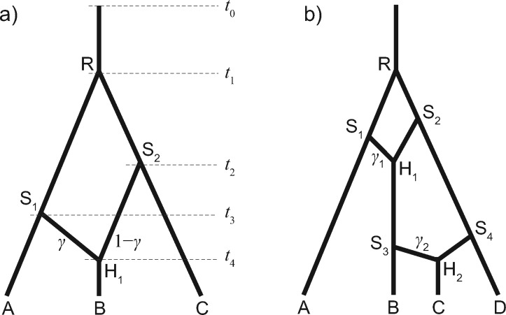
The birth-hybridization process provides a prior probability for a given species network Ψ (fig. 1). The process starts from t₀ (time of origin) in the past with a single species. A species gives birth to a new species with a constant rate λ (speciation rate), and two species merge into one with a constant rate ν (hybridization rate). That is, at the moment of k species, the speciation rate is $k\lambda$, the hybridization rate is $\left(\begin{array}{c}k\\ 2\end{array}\right)\nu$, and the waiting time to the next event is an exponential distribution. The process ends at time 0 (the present).

Fig. 1.

(a) A species network with three tips, three bifurcations, and one reticulation. The inheritance probability at branch S₁H₁ is γ, and that at $S_2{H}_1$ is $1-\gamma$. (b) Another network with four tips and two reticulations, with γ₁ and γ₂ associated with S₁H₁ and S₃H₂, respectively.

The probability density of a species network Ψ with n extant species descending from $n-1+m$ speciation events and m hybridization events, and these events happening at time $t_1>t_2>\dots >t_{n+2m-1}$, conditioned on t₀, λ and ν, is,

$$f(\Psi |\lambda ,\nu ,t_0)={\lambda }^{n+m-1}{\nu }^m\prod _{i=0}^{n+2m-1}{e}^{-\left(\lambda k_i+\nu (\begin{array}{c}{k}_i\\ 2\end{array})\right)(t_i-t_{i+1})},$$ (1)

where k_i is the number of lineages within time interval $(t_i,t_{i+1})$ and $t_{n+2m}=0$ is the present time. For the network shown in figure 1a, the probability density of the species network is

$$\begin{array}{c}f(\Psi |\lambda ,\nu ,t_0)=\lambda {\mathrm{e}}^{-\lambda (t_0-t_1)}\\ \lambda {\mathrm{e}}^{-(2\lambda +\nu )(t_1-t_2)}\\ \lambda {\mathrm{e}}^{-(3\lambda +3\nu )(t_2-t_3)}\\ \nu {\mathrm{e}}^{-(4\lambda +6\nu )(t_3-t_4)}\\ {\mathrm{e}}^{-(3\lambda +3\nu )t_4}.\end{array}$$

In our Bayesian analysis, the parameters λ, ν, and t₀ can be assigned hyperpriors.

Hybridizations or gene flow are modeled by reticulations in the species network. $\gamma =\{{\gamma }_1,\dots ,{\gamma }_H\}$ are the inheritance probabilities, one per reticulation node in Ψ (fig. 1). The inheritance probability measures the average proportion of genetic material inherited from the corresponding parent (or donor) (Long 1991; Yu et al. 2014; Wen and Nakhleh 2017). While the prior for $\gamma$ can be any distribution on $[0,1]$, in this study we use $f({\gamma }_h)\sim U(0,1)$ throughout.

The Probability Density of the Gene Trees Given the Species Network

The gene trees $G=\{G_1,G_2,\dots ,G_L\}$ are embedded in the species network Ψ under the MSNC model (Yu et al. 2014) (fig. 2). The effective population sizes $N=\{N_1,N_2,\dots ,N_B\}$ are assumed to be identically and independently distributed (i.i.d.) for each of the B branches in Ψ, while each locus has the same effective population size N_i at branch i ($i=1,\dots ,B$). For each locus j, the number of coalescences of gene tree G_j within branch b of Ψ is denoted by k_jb, and the number of lineages at the tipward end of b is denoted by n_jb, thus the number of lineages at the rootward end of b is $n_{jb}-k_{jb}$. The $k_{jb}+1$ coalescent time intervals between the tipward and rootward of branch b are denoted by c_jbi$(0\le i\le k_{jb})$. p_j is the gene ploidy of locus j (e.g., 2 for autosomal nuclear genes and 0.5 for mitochondrial genes in diploid species). For each lineage of G_j traversing the reticulation node H_h backward in time, with probability γ_h it goes to the parent branch associated with that inheritance probability, and to the alternate parent branch with probability $1-{\gamma }_h$. The corresponding number of traversing lineages are denoted by u_jh and v_jh, respectively.

Fig. 2.

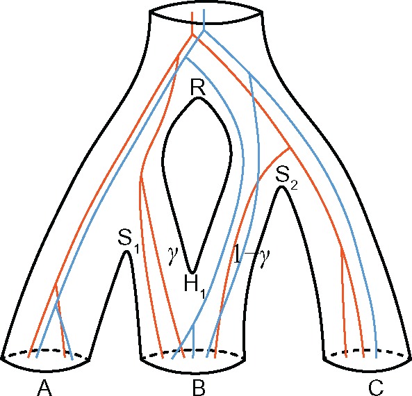
Two gene trees embedded in the species network of figure 1a. There are two samples from species A, three samples from B, and either one or two samples from C. For each gene tree lineage traversing the reticulation node H₁ backward in time, it goes to the left population with probability γ, and to the right with probability $1-\gamma$.

The coalescent probability of the gene trees G in species network Ψ with time being measured in calendar units is thus:

$$\begin{array}{c}f(G|\Psi ,\gamma ,N)=\prod _{j=1}^L[\prod _{b=1}^B{(p_j{N}_b)}^{-k_{jb}}\hspace{0.17em}\text{exp}\hspace{0.17em}(-{(p_j{N}_b)}^{-1}\sum _{i=0}^{k_{jb}}{c}_{jbi}(\begin{array}{c}{n}_{jb}-i\\ 2\end{array}))\prod _{h=1}^H{\gamma }_h^{u_{jh}}{(1-{\gamma }_h)}^{v_{jh}}]\\ =\Lambda \prod _{b=1}^B{r}_b{N}_b{-}^{q_b}\hspace{0.17em}\text{exp}\hspace{0.17em}(-{\sigma }_b{N}_b^{-1}),\end{array}$$ (2)

where $q_b=\sum _j{k}_{jb},\hspace{0.17em}{r}_b=\prod _j{p}_j^{-k_{jb}},\hspace{0.17em}{\sigma }_b=\sum _j{p}_j^{-1}\sum _{i=0}^{k_{jb}}{c}_{jbi}(\begin{array}{c}{n}_{jb}-i\\ 2\end{array})$, and $\Lambda =\prod _j\prod _h{\gamma }_h^{u_{jh}}{(1-{\gamma }_h)}^{v_{jh}}$. When there is no reticulation in the species network (i.e., it is a species tree), then Λ = 1 and equation (2) is equivalent to equation (2) in Jones (2017).

Integrating Out the Population Sizes Analytically

Equation (2) has the form of unnormalized inverse gamma densities. The population sizes N can be integrated out through the use of i.i.d. inverse-gamma(α, β) conjugate prior distributions (Hey and Nielsen 2007; Jones 2017), that is,

$$\begin{array}{c}f(G|\Psi ,\gamma )=\int f(G|\Psi ,\gamma ,N)f(N|\alpha ,\beta )\mathrm{d}N\\ =\Gamma \prod _{b=1}^B{\int }_0^{\infty }{r}_b{N}_b{-}^{q_b}\hspace{0.17em}\text{exp}\hspace{0.17em}(-{\sigma }_b{N}_b^{-1})\frac{{\beta }^{\alpha }}{\Gamma (\alpha )}{N}_b^{-\alpha -1}\hspace{0.17em}\text{exp}\hspace{0.17em}(-\beta N_b^{-1})\mathrm{d}{N}_b\\ =\Gamma \prod _{b=1}^B\frac{r_b{\beta }^{\alpha }}{{(\beta +{\sigma }_b)}^{\alpha +q_b}}\frac{\Gamma (\alpha +q_b)}{\Gamma (\alpha )}.\end{array}$$ (3)

The symbolic notations follow equation (2).

The Probability of the Sequence Data Given the Gene Trees

Assuming complete linkage within each locus, the probability of the data $D=\{D_1,D_2,\dots ,D_L\}$ given gene trees $G=\{G_1,G_2,\dots ,G_L\}$ is the product of phylogenetic likelihoods (Felsenstein 1981) at individual loci:

$$\mathrm{Pr}(D|G,\mu ,\varphi )=\prod _{i=1}^L\mathrm{Pr}(D_i|G_i,{\mu }_i,{\varphi }_i),$$ (4)

where G_i is the gene tree with coalescent times, μ_i is the substitution rate per site per time unit, and ${\varphi }_i$ represents the parameters in the substitution model (e.g., the transition–transversion rate ratio κ in the HKY85 model; Hasegawa et al. 1985), at locus i ($i=1,\dots ,L$).

There are two sources of evolutionary rate variation: across gene tree lineages at the same locus and across different gene loci. In the strict molecular clock model (Zuckerkandl and Pauling 1965), μ is the global clock rate, that is, no rate variation across gene lineages at each locus. To extend to a relaxed molecular clock model (e.g., Thorne and Kishino 2002; Drummond et al. 2006; Lepage et al. 2007; Rannala and Yang 2007), the molecular clock rate is variable across gene lineages following certain distributions with μ as the mean. To account for rate variation across genes, gene-rate multipliers $\{m_1,m_2,\dots ,m_L\}$ are constrained to average to 1.0 ($\sum _{i=1}^L{m}_i{x}_i=1$, where x_i is the proportion of sites in locus i to the total number of sites). Then the substitution rate at locus i is ${\mu }_i=\mu m_i$. Thus, when multiplying the gene tree lineages in G_i by μ_i, all the branch lengths are then measured in units of expected substitutions per site.

The gene-rate multipliers are assigned a flat Dirichlet prior. The average substitution rate (clock rate) μ can be either fixed to 1.0 such that branch lengths are measured by expected substitutions per site, or assigned an informative prior to infer branch lengths measured in absolute time. Note here, when time is measured by expected substitutions per site, we use ${\theta }_b=N_b\mu$ as the population size parameter of branch b, and ${\tau }_i=t_i\mu$ as the height of node i.

The Joint Posterior Distribution

The joint posterior distribution of the parameters is:

$$\begin{array}{c}f(\Psi ,G,\Theta |D)\propto \mathrm{Pr}(D|G,\mu ,\varphi )f(G|\Psi ,\gamma )f(\Psi |\lambda ,\nu ,t_0)\\ f(\mu )f(\varphi )f(\gamma )f(\lambda ,\nu )f(t_0).\end{array}$$ (5)

Here, Θ represents $(\mu ,\varphi ,\gamma ,\lambda ,\nu ,t_0)$.

Simulations

We investigate the performance of the implementation using simulations in this section. Time is measured by expected substitutions per site throughout the simulations, so that $\theta =N\mu$ is used for all population sizes and ${\tau }_i=t_i\mu$ for the time of node i. The substitution rate μ is fixed to 1.0 across all gene lineages (strict molecular clock) and all loci (no rate variation).

Simulation and MCMC Sampling without Sequence Data

To verify the implementation of our Bayesian MCMC method, we compared stochastic simulation to MCMC sampling of species networks and gene trees. We first generated networks under the birth-hybridization process. The simulator starts from the time of origin (t₀) with one species. A species splits into two (speciation) with rate λ, and two species merge into one (hybridization) with rate ν. At the moment of k branches, the total rate of change is $r_{tot}=k\lambda +(\begin{array}{c}k\\ 2\end{array})\nu$. We generate a waiting time $\sim \hspace{0.17em}\text{exp}\hspace{0.17em}(r_{tot})$ and a random variable $u\sim U(0,1)$. If $u<k\lambda /r_{tot}$, we randomly select a branch to split; otherwise, we randomly select two branches to join, and generate an inheritance probability $\gamma \sim U(0,1)$. The simulator stops at time 0 (cf. fig. 1). In this simulation, ${\tau }_0=0.1,\hspace{0.17em}\lambda =20,\nu =10$, and we kept 200,000 networks with exactly three tips. All the population sizes were fixed to $\theta =0.01$. Given each simulated species network, we then simulated a gene tree with two samples from each species (2, 2, 2) under the backward-in-time MSNC, resulting in 200,000 gene trees.

In the MCMC, we used all the operators for the species network (with three tips), gene tree (with two samples per species), and embedding (see above). The parameters ${\tau }_0,\lambda ,\nu$ and θ were fixed to the truth. The likelihood of data was set to be constant (no data). The chain was run 500 million steps and sampled every 2000 steps. The last 200,000 sampled species networks and gene trees were kept (i.e., the burn-in was 20%).

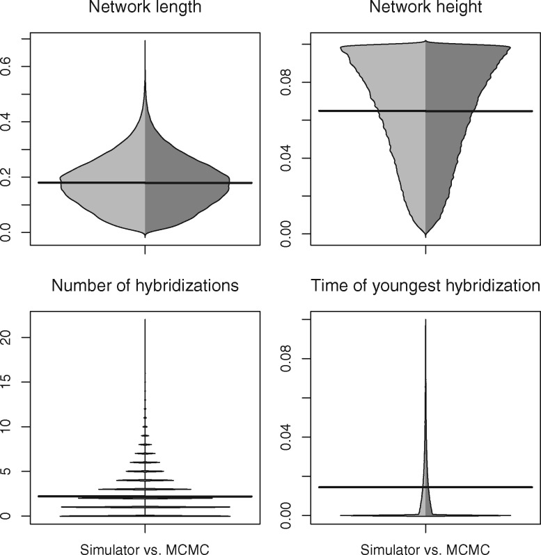
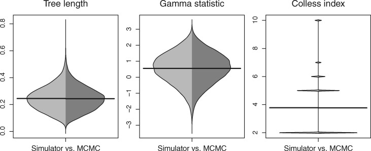
Theoretically, we expect the distributions of species network and gene trees to be identical from both simulation and MCMC sampling. Indeed, the networks obtained from the simulator and MCMC match when comparing the network length, root height, number of hybridizations, and time of the youngest hybridization (fig. 3). The tree sets from MSNC and MCMC also give rise to the same distributions of tree length, the gamma-statistic (Pybus and Harvey 2000), and Colless index (Blum et al. 2006) as expected (fig. 4).

Fig. 3.

Beanplot of network summary statistics comparing 3-tips networks simulated under the birth-hybridization process (left, light gray) with those sampled using the MCMC operators (right, dark gray). The horizontal bar is the mean.

Fig. 4.

Beanplot of three tree summary statistics comparing gene trees simulated under MSNC (left, light gray) with those sampled using the MCMC operators (right, dark gray). The sample configuration was (2, 2, 2).

Inference of Species Networks from Sequences

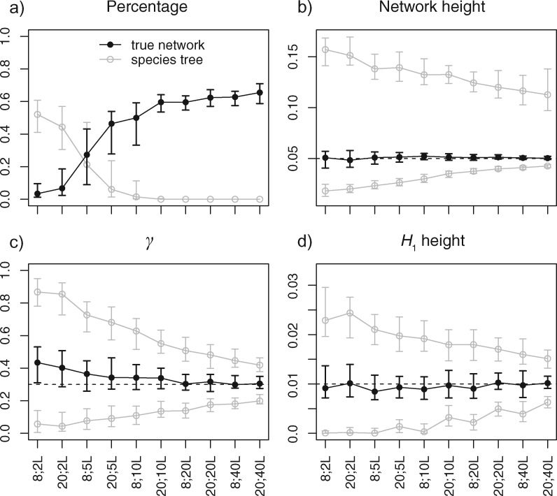
We simulated sequence alignments of multiple loci to reveal the ability of our method to recover the true species network from multilocus sequence data. The true network is shown in figure 1a, with ${\tau }_1=0.05,{\tau }_2=0.03,{\tau }_3=0.02,{\tau }_4=0.01,\gamma =0.3$, and population sizes $\theta =0.01$. A random gene tree was generated for each locus under the MSNC. Then DNA sequences of length 200 bp were simulated under JC69 model (Jukes and Cantor 1969) along each tree. The sample configurations were (2, 4, 2) (meaning species A has 2, B has 4, and C has 2 sampled sequences) and (5, 10, 5), and the number of loci was 2, 5, 10, 20, 40, respectively. Under each setting, the simulation was repeated 100 times. In the inference, the priors were ${\tau }_0\sim$ exp(10) with mean 0.1, $d=\lambda -\nu \sim$ exp(0.1) with mean 10, $r=\nu /\lambda \sim U(0,1)$, and $\gamma \sim U(0,1)$. The population sizes were integrated out analytically using inverse-gamma(5, 0.05) (eq. 3). The substitution model was set to JC69 (the true model). We fixed $\mu =1.0$ for all genes as in the simulation (strict molecular clock and no rate variation). The MCMC chain was run for 50 million steps and sampled every 2000 steps. The first 35% of samples were discarded as burn-in. The results are shown in figure 5.

Fig. 5.

Posterior estimates of (a) probability of the true network (black) and species trees (gray), (b) network height, (c) γ in the true network topology, and (d) H₁ height in the true network topology, when the data were simulated under the network in figure 1a with sample configuration (2, 4, 2) or (5, 10, 5), and 2, 5, 10, 20, or 40 loci, respectively. For each setting in (a), the dot/circle with error bars are the median and the first and third quartiles of the percentages of 100 replicates. For each setting in (b), (c), and (d), the black dot with error bars are the median and the first and third quartiles of the posterior medians of 100 replicates, the gray circles with error bars are the same summaries for the 95% HPD intervals. The dashed lines indicate the true values.

With only two loci, the species trees are inferred with the highest posterior probability, the distribution of species network topologies is sensitive to the prior (fig. 5a). The HPD intervals of the network height are also very wide (fig. 5b). As sample size increases, the posterior estimates become increasingly accurate. Conditional on the true species network topology inferred (i.e., fig. 1a), the estimates of inheritance probability γ and time of hybridization become increasingly accurate as the number of loci increases (fig. 5c and d). We also observe that adding loci increases the accuracy of inference more than adding individuals. For example, by comparing (5, 10, 5) individuals × 5 loci with (2, 4, 2) individuals × 10 loci, the latter has higher probability of recovering the true species network (fig. 5a).

To reveal the power of our method to detect both ancient and recent hybridization events, we simulated gene trees and sequences subsequently under the true species network shown in figure 1b, with ${\tau }_R=0.05,{\tau }_{H_1}=0.03,{\gamma }_1=0.6,{\tau }_{H_2}=0.01,{\gamma }_2=0.7,{\tau }_{S_1}=0.035,{\tau }_{S_2}=0.04,{\tau }_{S_3}=0.012,{\tau }_{S_4}=0.015$, and population sizes $\theta =0.01$. The sample configurations were (2, 2, 2, 2) and (5, 5, 5, 5), respectively. The other settings were kept the same as in the previous simulation. The results are shown in figure 6.

Fig. 6.

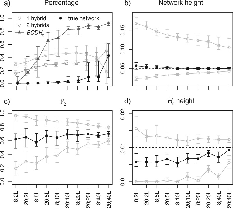
Posterior estimates of (a) probability of the true network (black), networks with one or two hybridizations (light gray), and networks with the BCDH₂ subnetwork (dark gray), (b) network height, (c) γ₂ in the BCDH₂ subnetwork, and (d) H₂ height in the BCDH₂ subnetwork, when the data were simulated under the network in figure 1b with sample configuration (2, 2, 2, 2) or (5, 5, 5, 5), and 2, 5, 10, 20, or 40 loci, respectively. For each setting in (a), the dot/circle with error bars are the median and the first and third quartiles of the percentages of 100 replicates. For each setting in (b), (c), and (d), the black dot with error bars are the median and the first and third quartiles of the posterior medians of 100 replicates, the gray circles with error bars are the same summaries for the 95% HPD intervals. The dashed lines indicate the true values.

We find that an ancient hybridization close to the root is much harder to detect than a recent hybridization. With up to 8 samples and 20 loci, the posterior probabilities of the true network topology are all close to zero. The estimates start to increase with 20 samples and 20 loci or more (fig. 6a). The difficulty is mainly due to the fact that there are few gene-tree lineages close to the root of the network, making it hard to distinguish the true hybridization event from incomplete lineage sorting in the ancestral populations. However, the recent hybridization event is inferred with high probability using 10–40 loci (fig. 6a). More specifically, we looked at the posterior probability of networks having the BCDH₂ subnetwork structure (cf. fig. 1b). Conditional on having this subnetwork inferred, the estimates of inheritance probability γ₂ become increasingly accurate as the number of loci increases (fig. 6c), although the time of hybridization H₂ is generally underestimated (fig. 6d). It is not feasible to perform larger scale simulations, for example, using 100 loci or more, to investigate the power of recovering the ancient hybridization (thus the true species network). Further studies need to be carried out after the efficiency of the operators is improved (see Discussion).

Analysis of Biological Data

Three Closely Related Spruce Species

We analyzed a data set of three spruce species (Picea purpurea, P. likiangensis, and P. wilsonii) in the Qinghai-Tibet Plateau (Sun et al. 2014). Piceapurpurea was inferred to be a homoploid hybrid of P. likiangensis and P. wilsonii (Sun et al. 2014). The original data have 11 nuclear loci and 166 diploid individuals (50 from P. wilsonii, 56 from P. purpurea, 60 from P. likiangensis, and two phased haplotype sequences per individual per locus).

To achieve proper mixing and convergence in a reasonable time, the data were truncated into two nonoverlapping data sets by randomly selecting individuals, resulting in 20 individuals from P. purpurea, 15 from P. likiangensis, and 15 from P. wilsonii (100 sequences per locus) for each. The priors for the species network were ${\tau }_0\sim$ exp(500) with mean 0.002, $d=\lambda -\nu \sim$ exp(0.01) with mean 100, $r=\nu /\lambda \sim U(0,1)$, and $\gamma \sim U(0,1)$. The population sizes were integrated out analytically (eq. 3) using inverse-gamma(3, 0.003) with mean 0.0015 and mode 0.00075. The substitution model was HKY85 (Hasegawa et al. 1985), with independent κ (transition–transversion rate ratio) and state frequencies at each locus. The clock rate was fixed to 1.0 (strict molecular clock across branches) and gene-rate multipliers were used to account for rate variation across loci. The MCMC chain was run for 1 billion steps and sampled every 20,000 steps. The first 35% of samples were discarded as burn-in. For each data set, we obtained two independent runs, and the two runs were checked for effective sample sizes (ESS) and the consistency of trace plots of inferred parameters. The MCMC samples from the two runs were combined.

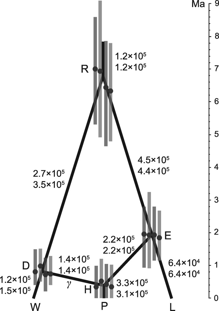
The species network shown in figure 7 has a posterior probability >0.95 for both data sets. This confirms that P. purpurea is a hybrid species of P. likiangensis and P. wilsonii. The estimates of γ are 0.33 (0.18, 0.52) and 0.37 (0.17, 0.57), respectively (median and 95% HPD interval). To investigate the impact of prior on population sizes, we fixed the species network topology to the one in figure 7, and used three priors for the population size parameter: inverse-gamma(3, 0.0003) with mean 0.00015 (small), inverse-gamma(3, 0.003) with mean 0.0015 (medium), and inverse-gamma(3, 0.03) with mean 0.015 (large), respectively. The population sizes were either inferred using MCMC or integrated out analytically. The other priors and MCMC settings were unchanged.

Fig. 7.

The species network with highest posterior probability ($>95\%$) inferred from the spruce data. The medians and 95% HPD intervals of node heights (black dots with error bars) are in unit of million years. From left to right, they are for data set 1 with population sizes inferred and integrated out, and data set 2 with population sizes inferred and integrated out, under the inverse-gamma(3, 0.003) prior. The numbers beside the branches are the medians of effective population sizes inferred from data set 1 (above) and 2 (below). See also supplementary tables S1 and S2, Supplementary Material online.

The posterior estimates of γ, node heights, and population sizes are summarized in supplementary tables S1 and S2, Supplementary Material online. The estimates are similar for both data sets regardless of whether the population sizes were inferred or integrated out under the same prior, but some estimates vary slightly across different priors. Below we summarize the results from the inverse-gamma(3, 0.003) prior (medium mean) for population sizes (fig. 7, and middle column of supplementary tables S1 and S2, Supplementary Material online). Around 31–37% of the nuclear genome of P. purpurea was derived from P. wilsonii (and thus 63–69% from P. likiangensis). This estimate is concordant with the original estimate of 31% made using approximate Bayesian computation (ABC) (Sun et al. 2014). Assuming an average substitution rate $\mu =2\times {10}^{-4}$ per site per million years (Sun et al. 2014), and dividing the node heights (τ’s in supplementary tables S1 and S2, Supplementary Material online) by μ, we get the times measured by million years (fig. 7). The time of hybridization is inferred to be around 1 Ma. The estimate was 1.3 (0.73, 2.2) Ma in the original analysis assuming the same height for nodes D, E, and H. Moreover, we get an older and narrower estimate for the root age (fig. 7), compared with 2.7 (1.4, 6.5) Ma in the original analysis. Similarly, dividing estimates of θ’s (supplementary tables S1 and S2, Supplementary Material online) by $\mu =1\times {10}^{-8}$ per site per generation, we get the effective population sizes (fig. 7). The inferred population sizes of P. purpurea, P. wilsonii, and P. likiangensis are smaller than those estimated using ABC (cf. table 4 in Sun et al. 2014).

Seven Yeast Species (Saccharomyces)

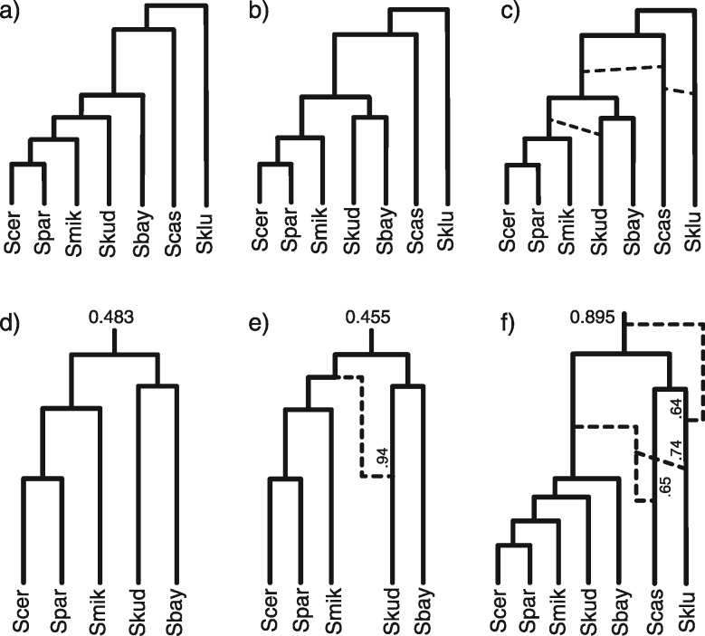
We reanalyzed another data set of seven yeast species, including S. cerevisiae (Scer), S. paradoxus (Spar), S. mikatae (Smik), S. kudriavzevii (Skud), S. bayanus (Sbay), S. castellii (Scas), and S. kluyveri (Sklu). There are in total 106 orthologous gene loci and one sequence per species per locus (Rokas et al. 2003). This data analyzed using concatenation under maximum likelihood yielded a single tree (fig. 8a) with 100% bootstrap values at every branch (Rokas et al. 2003). The analysis using BEST (Liu 2008) showed two main species trees in the posterior (fig. 8a and b) (Edwards et al. 2007). Both studies discovered extensive incongruent phylogenies from individual genes, with phylogenetic conflict often involving Scas and Sklu. Recently, the full data set was also analyzed using a Bayesian method coestimating species networks and gene trees. Extensive hybridization events were found, usually involving Scas and Sklu as the donor or recipient (Wen and Nakhleh 2017).

Fig. 8.

The species networks inferred from the yeast data. (a) The species tree estimated using concatenation under maximum likelihood (Rokas et al. 2003). (a) and (b) are the two main species trees in the posterior analyzed using BEST (Edwards et al. 2007). (c) The representative species network inferred using our method on all seven species and 106 loci. The dashed lines indicate possible hybridization events. (d) and (e) are two species networks in the 95% posterior credible set using five species and 106 loci (excluding Scas and Sklu). The posterior probabilities are labeled at the root. (f) The species network inferred using seven species and 28 loci with the strongest phylogenetic signal. The larger inheritance probabilities are labeled beside the corresponding branches.

For the inference using our method, the priors for the species network were ${\tau }_0\sim$ exp(10) with mean 0.1, $d=\lambda -\nu \sim$ exp(0.2) with mean 5, $r=\nu /\lambda \sim U(0,1)$, and $\gamma \sim U(0,1)$. The population sizes were integrated out analytically with the prior inverse-gamma(3, 2θ), while the mean population size θ was assigned a gamma(2, 100) prior, which has a mean of 0.02. We still used the HKY85 substitution model (Hasegawa et al. 1985), gene-rate multipliers for rate variation across loci, and the same MCMC chain settings as in the spruce data analysis.

Similarly, we observed extensive hybridizations among Scas, Sklu, and the remaining five species (fig. 8c) in the posterior estimates from independent runs. The incongruence among gene tree phylogenies are well captured and explained by the hybridization events. These patterns are similar to the results in Wen and Nakhleh (2017). The backbone tree (by removing the reticulation branches with smaller inheritance probabilities from the networks) is consistent with the species tree in figure 8b. However, the complexity of hybridizations caused difficulty and poor mixing of MCMC using the full data. The species network topology may stay unchanged for long durations of the MCMC chain and independent runs give different numbers and directions of hybridizations, although the hybridization pattern and the backbone tree are the same across runs.

Using only five species by excluding Scas and Sklu produced consistent results across runs, and the posterior samples from the three runs are combined. About half of the samples in the 95% posterior credible set are species trees (fig. 8d) and another half are species networks with one reticulation leading to Skud (fig. 8e). The result of Wen and Nakhleh (2017, fig. 22e) showed only one species network in the 95% posterior credible set with opposite hybridization direction (from Skud to Sbay) and smaller γ then ours (0.75 vs. 0.94). But both analyses have the same backbone tree as in figure 8d. The difference is probably due to the different priors and evolutionary models we used (see Discussion). The inheritance probability of 0.94 is fairly high, such that only a small amount of genes in Skud are horizontally transferred from the ancestral species of Smik. Thus, we do not interpret Skud as a hybrid species between Sbay and the ancestral species of Smik. Further investigations are needed to fully understand the underlining biological mechanism. The root heights are both 0.094 (0.092, 0.096) (median and 95% HPD interval) in figure 8d and e. The branch lengths are measured by the mean substitutions per site. The posterior estimate of mean population sizes θ is 0.00086 (0.00015, 0.0018). The rate multipliers range from 0.55 to 1.5 for the 106 loci, indicating small amount of evolutionary rate variation among loci.

We further investigated the 28 loci with the strongest phylogenetic signal. The gene trees inferred from these loci under maximum likelihood have at least four internal branches with bootstrap support $>70\%$ (Nakhleh L, personal communication). The priors and MCMC settings are the same as for the 106 loci. Using all the seven species, the species network with highest posterior probability (0.895) is shown in figure 8f. Three hybridization events are recovered, two from an ancestor of Saccharomyces sensu stricto (Scer, Spar, Smik, Skud, and Sbay) into Scas and Sklu. In addition, we found a hybridization event deriving from an ancestral species of sampled extant Saccharomyces. When using only five species by excluding Scas and Sklu in a separate run, the species tree with the same topology as the subtree in figure 8f was inferred with highest posterior probability (0.98). This is different from the backbone tree using all 106 loci (cf. fig. 8d), indicating conflicting phylogenetic signal among loci.

Materials and Methods

We now describe the MCMC operators in detail and an algorithm to summarize networks sampled from the MCMC, followed by a convenient format for the networks and a link to our source code.

MCMC Operators for the Species Network

Node Slider

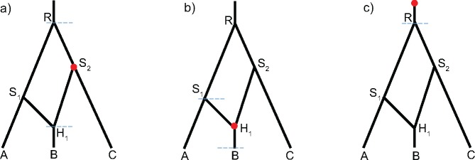
The node-slider operator only changes the node heights of the species network, not the topology. It selects an internal node or the origin randomly, then proposes a new height centered at the current height according to a normal distribution: $t\prime |t\sim N(t,{\sigma }^2)$, where σ is a tuning parameter controlling the step size. The lower bound is the oldest child-node height, the upper bound is the youngest parent-node height (except for the origin, fig. 9). If the proposed value is outside this range, the excess is reflected back into the interval. Note that for the origin, if the proposed height is outside the range of its prior, this move is aborted. A variation of this operator can use a uniform proposal instead of the normal proposal: $t\prime |t\sim U(t-w/2,t+w/2)$, where w is the window size. The proposal ratio is 1.0 in both cases.

Fig. 9.

Three cases when the node-slider operator is applied: (a) a bifurcation node S₂ is selected; (b) the reticulation node H₁ is selected; and (c) the origin is selected. The dashed lines are the lower and upper bounds for changing its height (only the lower bound is applicable in c). For the node-uniform operator, (a) and (b) apply but (c) does not.

Node Uniform

The node-uniform operator also changes the internal-node heights of the species network while keeping the topology. It selects an internal node randomly, then proposes a new height uniformly between the lower and upper bounds (fig. 9a and b). The lower bound is the oldest child-node height, the upper bound is the youngest parent-node height. The proposal ratio is 1.0. Unlike node slider, this operator does not change the time of origin. A separate operator for the origin, such as multiplier or scaler, can be coupled to update all the node heights.

Relocate Branch

The relocate-branch operator can change the topology, but keeps the number of reticulations in the species network constant. It first selects an internal node at random. If the selected node is a bifurcation node, the rootward end of either its child branches is selected (fig. 10a); if the selected node is a reticulation node, the tipward end of either its parent branches is selected (fig. 10b). Then the selected branch is detached at the side of the selected node, and a destination branch to be attached is chosen randomly from all possible candidate branches (including the original position). A new height of the selected node is proposed uniformly between the heights of the two ends of the destination branch ($v\prime$ and $u\prime$ in fig. 10). When the relocated branch has a bifurcation node at one end and a reticulation node at the other end, the candidate branches include all the remaining branches, and the reticulation direction can be changed depending on the proposed new height (fig. 10b). When the relocated branch has the same type of nodes at both ends and the resulted network is invalid, the move is aborted. For example, moving the rootward end lower than the tipward end if the two ends are both bifurcation nodes, or moving the tipward end higher than the rootward end if the two ends are both reticulation nodes, will result in an invalid network. We denote with v and u the lower and upper bounds of the backward move. The proposal ratio is $(u\prime -v\prime )/(u-v)$.

Fig. 10.

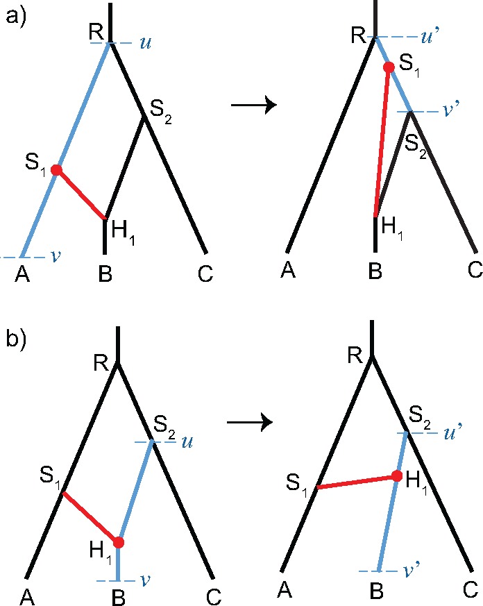
Two cases when the relocate-branch operator is applied. (a) A bifurcation node S₁ is selected, and branch S₁H₁ is relocated to attach to RS₂. (b) A reticulation node H₁ is selected, and branch S₁H₁ is still attaching to $S_{2}B$ with flipped reticulation direction. The lower and upper bounds of proposing the new attaching point are $v\prime$ and $u\prime$, and the corresponding bounds of the backward move are v and u.

Add- and Delete-Reticulation

The add-reticulation and delete-reticulation operators are reversible-jump MCMC (rjMCMC) proposals that can add and delete a reticulation event, respectively.

In the add-reticulation operator, a new branch is added by connecting two randomly selected branches with length l₁ and l₂ (fig. 11). The same branch can be selected twice so that l₁ = l₂ (fig. 11b). Then three values ${\omega }_1,{\omega }_2$ and ω₃ are drawn from U(0, 1). One attaching point cuts the branch length l₁ to $l_{11}=l_1{\omega }_1$ (and thus $l_{12}=l_1(1-{\omega }_1)$); the other attaching point cuts the branch length l₂ to $l_{21}=l_2{\omega }_2$ (and thus $l_{22}=l_2(1-{\omega }_2)$). Analogously, if we select the same branch twice, the attachment times of the new branch are $l_1{\omega }_1$ and $l_1{\omega }_2$. An inheritance probability $\gamma ={\omega }_3$ is associated to the new branch. We will operate on the inheritance probability γ of this added branch, while the inheritance probability of the second reticulation branch (i.e., $1-\gamma$) changes accordingly. We denote k as the number of branches in the current network, and m as the number of reticulation branches (parent branches of the reticulation nodes) in the proposed network. The Hastings ratio is then $(1/m)/[(1/k)(1/k)\times 1\times 1\times 1]=k^2/m$. The Jacobian is $\left|\frac{\partial (l_{11},l_{21},\gamma )}{\partial ({\omega }_1,{\omega }_2,{\omega }_3)}\right|=l_1{l}_2$. Thus, the proposal ratio of add-reticulation is $l_1{l}_2{k}^2/m$.

Fig. 11.

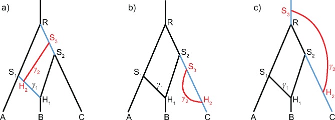
Three cases when the add-reticulation operator is applied. The number of branches in the current network (i.e., the network without the red branch) is k = 8. The probability of selecting the illustrated branches (in blue) is $1/k^2$. The number of reticulation branches in the proposed network is m = 4. In the reverse move, delete-reticulation, the probability of selecting the added branch (in red) is $1/m$. (a) Branches S₁H₁ and RS₂ are selected and a new branch S₃H₂ is added together with γ₂. The length of S₁H₁ is $l_1=l_{S_1{H}_1}$, and that of RS₂ is $l_2=l_{R{S}_2}$. In the delete-reticulation move, if $H_1{H}_2$ is selected, the operator is aborted. (b) The same branch S₂C is selected twice. $l_1=l_2=l_{S_{2}C},l_{11}=l_{S_2{S}_3},l_{21}=l_{S_2{H}_2}$. (c) The root branch and S₂C are selected. S₃ becomes the new root.

In the delete-reticulation operator, a random reticulation branch together with the inheritance probability γ is deleted (fig. 11). Joining the singleton branches at each end of the deleted branch, resulting in two branches with length l₁ and l₂ completes the operator (l₁ = l₂ when forming a single branch, fig. 11b). If there is no reticulation, or the selected branch is connecting two reticulation nodes, the move is aborted. For example, in figure 11a, deleting reticulation branch $H_1{H}_2$ will result in an invalid network. We denote k as the number of branches in the proposed network, and m as the number of reticulation branches in the current network. The proposal ratio of delete-reticulation is $m/(k^2{l}_1{l}_2)$.

Inheritance-Probability Uniform

The inheritance-probability uniform operator selects a reticulation node randomly, and proposes a new value of the inheritance probability $\gamma \prime \sim U(0,1)$. The proposal ratio is 1.0.

Inheritance-Probability Random-Walk

The inheritance-probability random-walk operator selects a reticulation node randomly, and applies a uniform sliding window to the logit of the inheritance probability γ, that is $y\prime |y\sim U(y-w/2,y+w/2)$, where $y=\text{logit}(\gamma )=\hspace{0.17em}\text{log}\hspace{0.17em}(\gamma )-\hspace{0.17em}\text{log}\hspace{0.17em}(1-\gamma )$. Since the proposal ratio for the transformed variable y is 1.0, and $\frac{\mathrm{d}\gamma }{\mathrm{d}y}=\frac{\mathrm{d}}{\mathrm{d}y}\left[{\mathrm{e}}^y/(1+{\mathrm{e}}^y)\right]={\mathrm{e}}^y/{(1+{\mathrm{e}}^y)}^2$, the proposal ratio for the original variable γ is $\frac{\mathrm{d}\gamma \prime }{\mathrm{d}y\prime }/\frac{\mathrm{d}\gamma }{\mathrm{d}y}={\mathrm{e}}^{(y\prime -y)}{(1+{\mathrm{e}}^y)}^2/{(1+{\mathrm{e}}^{y\prime })}^2$.

MCMC Operators for Gene Trees

The standard tree operators in BEAST 2 (Bouckaert et al. 2014) are applied to update the gene trees, including the scale, uniform, subtree-slide, narrow- and wide-exchange, and Wilson–Balding (Wilson and Balding 1998). The scale and uniform operators only update the node heights without changing the tree topology, while the other operators can change the topology (Drummond and Bouckaert 2015). The species network is kept unchanged when operating on the gene trees, and vice versa.

MCMC Operator for the Gene Tree Embedding

The gene trees must be compatibly embedded in the species network (fig. 2). When a new gene tree is proposed using one of the tree operators, the rebuild-embedding operator proposes a new embedding for that gene tree. When a new species network is proposed, the rebuild-embedding operator proposes a new embedding for each gene tree in the species network. If there is no valid embedding for any gene tree, the gene tree or species network proposal is rejected.

The rebuild-embedding operator proposes a new embedding proportional to the product of traversal probabilities across all traversed reticulation nodes. Specifically, we define the (unnormalized) likelihood of a compatible embedding x as $w_x=\prod _{h=1}^H{\gamma }_h^{u_{xh}}{(1-{\gamma }_h)}^{v_{xh}}$, where H is the number of reticulation nodes in the species network, u_xh is the number of lineages traversing node H_h to the branch associated with γ_h, and v_xh is the number of lineages traversing node H_h to the alternative branch associated with $1-{\gamma }_h$. If there is no reticulation in the species network (i.e., it is a species tree), w_x = 1. For example, in figure 2, there are two possible embeddings for one gene tree (orange) while the likelihoods are ${\gamma }^2(1-\gamma )$ (current) and ${(1-\gamma )}^3$, respectively, and four possible embeddings for the other gene tree (blue) while the likelihoods are ${\gamma }^2,\hspace{0.17em}\gamma (1-\gamma ),\hspace{0.17em}(1-\gamma )\gamma$, and ${(1-\gamma )}^2$ (current), respectively.

The proposal ratio of moving from embedding x to $x\prime$ is:

$$\frac{w_x}{\sum _{i=1}^E{w}_i}/\frac{w_{x\prime }}{\sum _{j=1}^{E\prime }{w}_j},$$

where E and E′ are the number of possible embeddings in the current and new states, respectively. If $E\prime =0$ (no valid embedding), the move is aborted. This proposal distribution is chosen to have a superior acceptance ratio than if a new embedding is proposed randomly from all possible embeddings.

Summarizing Posterior Distribution of Species Networks

Reducing many hundreds of posterior or bootstrap samples to a summary result is essential in order to describe the underlying distribution. For phylogenetic trees, many summary methods have been developed such as “majority rule consensus” and “maximum clade credibility” trees (Heled and Bouckaert 2013). By comparison, methods to summarize samples of phylogenetic networks are underdeveloped. We have implemented a basic method for summarizing networks, where unique network topologies are reported in descending order of their posterior probabilities. For each unique topology, each subnetwork is annotated with its posterior probability and node age credible interval.

To facilitate the calculation of posterior probabilities and credible intervals, we have developed an algorithm to enumerate each unique subnetwork, and label all occurrences of a unique subnetwork in a sample of phylogenetic networks. After running this algorithm, the label of a network’s root node uniquely identifies its topology, and the generation of a sorted summary of posterior topologies becomes trivial. Details of the algorithm are given in the Appendix. The default setting of our summary tool eliminates all parallel branches (e.g., S₃H₂ in fig. 11b) from all samples in the posterior before summarizing, which simplifies the posterior distribution of networks and reduces the number of unique topologies.

Alternatively, users may generate a summary network using the “major displayed tree” method as implemented in the PhyloNetworks package (Solís-Lemus et al. 2017).

Representation of Phylogenetic Networks

Species networks are outputted in extended Newick format (Cardona et al. 2008), which is also used in the software PhyloNet (Than et al. 2008).

For example, the species network in figure 1a is written as:

((A: 0.02,(B: 0.01)#H1[&gamma = 0.3]: 0.01) S1: 0.03,

(#H1: 0.02, C: 0.03)S2: 0.02)R: 0.03;

where the hash sign indicates a reticulation node, and the inheritance probability is in the brackets as metadata. Such extended Newick string can be read into IcyTree (icytree.org; Vaughan 2017) and be displayed nicely.

Software Availability

The method is implemented in the add-on SpeciesNetwork for BEAST 2 (Bouckaert et al. 2014), including the inference, simulation, and summary tools, and is hosted publicly on GitHub (https://github.com/zhangchicool/speciesnetwork; last accessed December 10, 2017).

Discussion

We use species networks to model reticulate evolution. Although our method is motivated by species hybridization, species networks can also be applied to studies of migration and lateral (or horizontal) gene transfer. Rates of migration between taxa have been modeled previously using isolation-with-migration (IM) models (Nielsen and Wakeley 2001; Hey and Nielsen 2004, 2007; Wilkinson-Herbots 2008; Hey 2010; Zhu and Yang 2012; Dalquen et al. 2017). Reticulation branches in species networks can also model migration, and may be a more natural fit when migration is not constant as in the case of secondary contact. The proportion of genetic material inherited through a reticulation event can come from a high rate of migration over a short period of time, or a lower rate of migration over a longer period of time. Lateral gene transfer has been modeled previously using gene duplication, transfer, and loss (DTL) models (Tofigh et al. 2011; Szöllősi et al. 2012, 2013, 2015; Sjöstrand et al. 2014). These models account for discordance between species tree and gene trees by any discordance to DTL events, but ignore incomplete lineage sorting. Our implementation of species networks explicitly models the embedding of gene trees within a species network, and so can be used to infer lateral gene transfer events without confounding them with incomplete lineage sorting.

Methods to build a species network (e.g., Park et al. 2010; Wu 2010; Albrecht et al. 2012) traditionally use inferred gene trees from each locus without accounting for their uncertainties, and employ nonparametric criteria such as parsimony. For population level data, the sequences are similar and the signal in gene tree topologies is typically low, so using fixed gene trees is assigning too much certainty to the data. These methods typically assume that gene tree discordance is solely due to reticulation, thus may suffer in the presence of incomplete lineage sorting (Yu et al. 2011). The MSNC model (Yu et al. 2014) provides a statistical framework to account for both incomplete lineage sorting and reticulate evolution. But properly analyzing genetic data to infer species networks under the MSNC model is a challenging task. There have been methods using only the gene tree topologies from multiple loci under MSNC (Yu et al. 2012, 2014; Wen et al. 2016). However, gene trees with branch lengths are more informative for inferring species tree or network topology than gene tree topologies alone. Accounting for branch lengths can improve distinguishability of species networks (Pardi and Scornavacca 2015; Zhu and Degnan 2017). Although methods using estimated gene trees (with branch lengths) from bootstrap or posterior samples as input take into account gene tree uncertainty (Yu et al. 2014; Wen et al. 2016), directly using sequence data to coestimate species networks and gene trees in a Bayesian framework showed improved accuracy (Wen and Nakhleh 2017). Pseudo-likelihood approaches (Yu and Nakhleh 2015; Solís-Lemus and Ané 2016) compute faster than full likelihood or Bayesian approaches, but have severe distinguishability issues and require more data to achieve good accuracy.

At the time of writing, another Bayesian method inferring species networks and gene trees simultaneously from multilocus sequence data was released (Wen and Nakhleh 2017). The general framework here is similar, but we highlight four major differences. We use a birth-hybridization prior for the species network which naturally models the process of speciation and hybridization. The prior is extendable to account for extinction, incomplete sampling, and rate variation over time, as we outline below. Wen and Nakhleh (2017) used a descriptive prior combining a Poisson distributed number of reticulations with exponential distributed branch lengths. Secondly, we allow parallel branches in the network. This is biologically possible. Even if the true species history has no parallel branches, the observed species network can still contain such features due to incomplete sampling. Note though that a very large number of individuals and loci are required to detect such parallel branches. To prevent the species network from growing arbitrarily big, such that it becomes indistinguishable by the gene trees (Pardi and Scornavacca 2015; Zhu and Degnan 2017), we typically assign an informative prior to ensure the hybridization rate is lower than the birth rate. A similar strategy was used in Wen et al. (2016); Wen and Nakhleh (2017) by restricting the rate of the Poisson distribution. Third, we account for the uncertainty in the embedding of a gene tree within a species network by estimating the MSNC probability conditional on a proposed embedding at each MCMC step. This provides a posterior distribution of gene trees and their embeddings within a species network, enabling analysis of which alleles are derived from which ancestral species. The cost instead is additional MCMC operations compared with integrating over all embeddings at each step (Wen et al. 2016; Wen and Nakhleh 2017). Last but not least, we implement analytical integration over population sizes in the species network (eq. 3). This reduces the number of parameters for the rjMCMC operators to deal with, and should improve convergence and mixing. Finally, our implementation in SpeciesNetwork is an extension to BEAST 2 (Bouckaert et al. 2014), to take advantage of many standard phylogenetic models, such as different substitution models, relaxed molecular clock models, and the BEAUTi graphical interface.

In our approach, we employ a simple prior for the species network based on a birth-hybridization model. Analogous to birth-death priors for species trees (e.g., Stadler 2010; Heath et al. 2014), the birth-hybridization prior could be extended to account for extinction and incomplete sampling, to model networks containing both extant and fossil taxa. The rates could also be allowed to vary over time, to model the diversification patterns during speciation (the skyline model for trees, Stadler et al. 2013). When considering networks instead of trees, techniques to derive the probability density of trees cannot be directly applied as the hybridization rate depends on pairs of lineages rather than individual lineages. This nonlinearity necessitates solving differential equations to derive the species network probability densities, a task which we defer to a later study.

Our approach is limited in computational speed. The empirical analysis was done, for example, on only three species with 50 individuals and 11 loci, or up to seven species and 106 loci but one individual per species. The main bottleneck is the MCMC operators. Due to hard constraints between the species network and embedded gene trees (fig. 2), MCMC operators changing them separately limit the ability to analyze genomic scale data from many individuals. More specifically, updating the species network will likely violate a gene tree embedding, resulting in very low acceptance rate of the operator. Thus, it will be essential to design more efficient MCMC operators. There have been coordinated operators that can change species tree and gene trees simultaneously (Jones 2017; Rannala and Yang 2017). Such operators could possibly be extended to species networks, and will potentially improve efficiency of the MCMC algorithm. Proposing new embeddings of gene trees in species network is also costly. Thus, it might be worthwhile to integrate over the embeddings (Wen et al. 2016; Wen and Nakhleh 2017) if they are not of interest. Moreover, there are methods to integrate out the gene trees under the multispecies coalescent model when analyzing biallelic genetic markers (RoyChoudhury et al. 2008; Bryant et al. 2012; Zhu et al. 2017). However, it is not yet feasible to apply this strategy to multilocus sequence alignment. Computationally, implementing Metropolis-coupled MCMC (MC³, Geyer 1991) will help to overcome multiple local peaks in the posterior, and further parallelizing the cold and hot chains will gain speed.

In summary, we developed a Bayesian method for inferring species networks together with gene trees and evolutionary parameters from multilocus sequence data. The method is implemented within a general Bayesian framework, with potential future extensions to the theoretical model and to the practical implementation.

Supplementary Material

Supplementary data are available at Molecular Biology and Evolution online.

Appendix

Numbering and Labeling Subnetworks across a Sample

We describe an algorithm by pseudocode to enumerate all unique subnetwork topologies within a sample of phylogenetic networks. Apart from subnetwork topologies consisting of a single node (i.e., leaf nodes), each topology label has a corresponding set of child subnetwork topology numbers. The algorithm works by recursively constructing the mapping of parent to child subnetwork topology numbers, beginning at the root or origin node of each phylogenetic network.

Initialize the counter i to 0

Initialize the ({node label set} to node label) map m

For each taxon t :

  Assign i as the label of t

  Increment i

For each phylogenetic network s :

    Begin Recursion from the oldest node of s

Recursion:

  Input: A network node n

  Output: A label l to identify the subnetwork topology of n

  If n is a leaf node:

    Get the label l of the taxon t of n

  Else:

    Initialize the node label set d

      For each child node n _c of n :

        Get l _c by continuing Recursion from n _c

        Add l _c to d

    If d is in m :

        Get the label l of d

    Else:

        Set l to the value of i

        Link d to l in m

        Increment i

  Return l

Proposing Embeddings Proportional to Their Likelihoods

We describe an algorithm by pseudocode to propose compatible gene tree embeddings, given a species network and a set of gene trees, in proportion to their embedding likelihoods. The algorithm works by stochastically constructing an embedding during a depth-first search of a gene tree. When a gene tree lineage traverses a bifurcation node, there is a set of compatible embedding histories (for the subtree defined by the gene tree lineage) where the lineage descends through the left child branch of the bifurcation node, and another set for the right child branch. A left or right embedding is chosen at random weighted by the sum total of embedding likelihoods for each child branch of the bifurcation node, to ensure that embeddings are proposed in proportion to their likelihoods.

The likelihood for the proposed embedding is also computed during the depth-first search; when a gene tree lineage traverses a reticulation node, its likelihood is multiplied by the γ_h or the (alternative) 1−γ_h probability. When a coalescent event occurs, the likelihoods of the left and right subtrees are multiplied. Because embeddings are proposed in proportion to their likelihoods, the MCMC proposal probability is the embedding likelihood normalized by the sum total of compatible embedding likelihoods.

Given the species network s :

  For each gene tree g :

      Get the root gene tree node gtn _r from g

        Get the root species network branch snb _r from s

            Try to get e , l , and t by Recursion from gtn _r and snb _r

        If there is no compatible embedding:

          Reject the proposal

      Else:

                Propose e as the new embedding

              Multiply the proposal probability by ( $l÷t$ )

Recursion:

      Input 1: A gene tree node gtn

  Input 2: A species network branch snb

  Output 1: An embedding e

  Output 2: Its likelihood l

  Output 3: The total likelihood t

  If gtn traverses through the tipward node of snb :

      For each child branch snb _c of snb :

        If there is any compatible embedding of gtn through snb _c :

                  Get e _c , l _c , and t _c by Recursion from gtn and snb _c

                Add the traversal of gtn through snb _c to e _c

                If the tipward node of snb is a reticulation:

                  Multiply l _c by γ_hor 1−γ_h

                  Multiply t _c by γ_hor 1−γ_h

       Pick one snb _c at random weighted by t _c

         Set the embedding e to the value of e _c for the chosen snb _c

      Set the likelihood l to the value of l _c for the chosen snb _c

       Calculate the total likelihood t as the sum of all t _c

    Else:

          If gtn is a leaf:

            Initialize an embedding e

            Initialize the likelihood l to 1

            Initialize the total likelihood t to 1

          Else:

            For each child node gtn _c of gtn :

                Get e _c , l _c , and t _c by Recursion from gtn _c and snb

            Construct the embedding e by merging both e _c

            Calculate the likelihood l as the product of both l _c

              Calculate the total likelihood t as the product of both t _c

    Return e , l , and t

References

- Albrecht B, Scornavacca C, Cenci A, Huson DH.. 2012. Fast computation of minimum hybridization networks. Bioinformatics 282:191–197.http://dx.doi.org/10.1093/bioinformatics/btr618 [DOI] [PubMed] [Google Scholar]
- Blum MGB, François O, Janson S.. 2006. The mean, variance and limiting distribution of two statistics sensitive to phylogenetic tree balance. Ann Appl Probability 164:2195–2214. [Google Scholar]
- Bouckaert R, Heled J, Kühnert D, Vaughan T, Wu CH, Xie D, Suchard MA, Rambaut A, Drummond AJ.. 2014. BEAST 2: a software platform for Bayesian evolutionary analysis. PLoS Comput Biol. 104:e1003537.. [DOI] [PMC free article] [PubMed] [Google Scholar]
- Bryant D, Bouckaert R, Felsenstein J, Rosenberg NA, RoyChoudhury A.. 2012. Inferring species trees directly from biallelic genetic markers: bypassing gene trees in a full coalescent analysis. Mol Biol Evol. 298:1917–1932. [DOI] [PMC free article] [PubMed] [Google Scholar]
- Cardona G, Rosselló F, Valiente G.. 2008. Extended Newick: it is time for a standard representation of phylogenetic networks. BMC Bioinformatics 9:532. [DOI] [PMC free article] [PubMed] [Google Scholar]
- Dalquen DA, Zhu T, Yang Z.. 2017. Maximum likelihood implementation of an Isolation-with-Migration model for three species. Syst Biol. 663:379–398. [DOI] [PubMed] [Google Scholar]
- Drummond AJ, Bouckaert RR.. 2015. Bayesian evolutionary analysis with BEAST. Cambridge, UK: Cambridge University Press. [Google Scholar]
- Drummond AJ, Ho SYW, Phillips MJ, Rambaut A.. 2006. Relaxed phylogenetics and dating with confidence. PLoS Biol. 45:e88.. [DOI] [PMC free article] [PubMed] [Google Scholar]
- Edwards SV, Liu L, Pearl DK.. 2007. High-resolution species trees without concatenation. Proc Natl Acad Sci U S A. 10414:5936–5941. [DOI] [PMC free article] [PubMed] [Google Scholar]
- Felsenstein J. 1981. Evolutionary trees from DNA sequences: a maximum likelihood approach. J Mol Evol. 176:368–376.http://dx.doi.org/10.1007/BF01734359 [DOI] [PubMed] [Google Scholar]
- Geyer CJ. 1991. Markov chain Monte Carlo maximum likelihood In Keramidas EM, editor. Computing science and statistics: Proc. 23rd Symp. Interface. p. 156–163. Interface Foundation, Fairfax Station. [Google Scholar]
- Guindon S, Dufayard JF, Lefort V, Anisimova M, Hordijk W, Gascuel O.. 2010. New algorithms and methods to estimate maximum-likelihood phylogenies: assessing the performance of PhyML 3.0. Syst Biol. 593:307–321. [DOI] [PubMed] [Google Scholar]
- Hasegawa M, Kishino H, Yano T.. 1985. Dating of the human-ape splitting by a molecular clock of mitochondrial DNA. J Mol Evol. 222:160–174.http://dx.doi.org/10.1007/BF02101694 [DOI] [PubMed] [Google Scholar]
- Heath TA, Huelsenbeck JP, Stadler T.. 2014. The fossilized birth-death process for coherent calibration of divergence-time estimates. Proc Natl Acad Sci U S A. 11129:E2957–E2966. [DOI] [PMC free article] [PubMed] [Google Scholar]
- Heled J, Bouckaert RR.. 2013. Looking for trees in the forest: summary tree from posterior samples. BMC Evol Biol. 13:221.. [DOI] [PMC free article] [PubMed] [Google Scholar]
- Hey J. 2010. Isolation with migration models for more than two populations. Mol Biol Evol. 274:905–920.http://dx.doi.org/10.1093/molbev/msp296 [DOI] [PMC free article] [PubMed] [Google Scholar]
- Hey J, Nielsen R.. 2004. Multilocus methods for estimating population sizes, migration rates and divergence time, with applications to the divergence of Drosophila pseudoobscura and D. persimilis. Genetics 1672:747–760.http://dx.doi.org/10.1534/genetics.103.024182 [DOI] [PMC free article] [PubMed] [Google Scholar]
- Hey J, Nielsen R.. 2007. Integration within the Felsenstein equation for improved Markov chain Monte Carlo methods in population genetics. Proc Natl Acad Sci U S A. 1048:2785–2790. [DOI] [PMC free article] [PubMed] [Google Scholar]
- Jones G. 2017. Algorithmic improvements to species delimitation and phylogeny estimation under the multispecies coalescent. J Math Biol. 74(1–2):447–467.http://dx.doi.org/10.1007/s00285-016-1034-0 [DOI] [PubMed] [Google Scholar]
- Jukes TH, Cantor CR.. 1969. Evolution of protein molecules. In Munro HN, editor. Mamm Protein Metab. p. 21–123. New York: Academic Press. [Google Scholar]
- Lepage T, Bryant D, Philippe H, Lartillot N.. 2007. A general comparison of relaxed molecular clock models. Mol Biol Evol. 2412:2669–2680.http://dx.doi.org/10.1093/molbev/msm193 [DOI] [PubMed] [Google Scholar]
- Liu L. 2008. BEST: Bayesian estimation of species trees under the coalescent model. Bioinformatics 2421:2542–2543.http://dx.doi.org/10.1093/bioinformatics/btn484 [DOI] [PubMed] [Google Scholar]
- Liu L, Yu L, Kubatko L, Pearl DK, Edwards SV.. 2009. Coalescent methods for estimating phylogenetic trees. Mol Phylogenet Evol. 531:320–328.http://dx.doi.org/10.1016/j.ympev.2009.05.033 [DOI] [PubMed] [Google Scholar]
- Long JC. 1991. The genetic structure of admixed populations. Genetics 1272:417–428. [DOI] [PMC free article] [PubMed] [Google Scholar]
- Mallet J. 2005. Hybridization as an invasion of the genome. Trends Ecol Evol. 205:229–237.http://dx.doi.org/10.1016/j.tree.2005.02.010 [DOI] [PubMed] [Google Scholar]
- Mallet J. 2007. Hybrid speciation. Nature 4467133:279–283.http://dx.doi.org/10.1038/nature05706 [DOI] [PubMed] [Google Scholar]
- Nielsen R, Wakeley J.. 2001. Distinguishing migration from isolation: a Markov chain Monte Carlo approach. Genetics 1582:885–896. [DOI] [PMC free article] [PubMed] [Google Scholar]
- Pardi F, Scornavacca C.. 2015. Reconstructible phylogenetic networks: do not distinguish the indistinguishable. PLoS Comput Biol. 114:e1004135. [DOI] [PMC free article] [PubMed] [Google Scholar]
- Park H, Jin G, Nakhleh L.. 2010. Algorithmic strategies for estimating the amount of reticulation from a collection of gene trees. Proceedings of the 9th Annual International Conference on Computational Systems Biology 114–123.
- Pybus OG, Harvey PH.. 2000. Testing macro-evolutionary models using incomplete molecular phylogenies. Proc R Soc B Biol Sci. 2671459:2267–2272. [DOI] [PMC free article] [PubMed] [Google Scholar]
- Rannala B, Yang Z.. 2003. Bayes estimation of species divergence times and ancestral population sizes using DNA sequences from multiple loci. Genetics 1644:1645–1656. [DOI] [PMC free article] [PubMed] [Google Scholar]
- Rannala B, Yang Z.. 2007. Inferring speciation times under an episodic molecular clock. Syst Biol. 563:453–466.http://dx.doi.org/10.1080/10635150701420643 [DOI] [PubMed] [Google Scholar]
- Rannala B, Yang Z.. 2017. Efficient Bayesian species tree inference under the multispecies coalescent. Syst Biol. 665:823–842. [DOI] [PMC free article] [PubMed] [Google Scholar]
- Rokas A, Williams BL, King N, Carroll SB.. 2003. Genome-scale approaches to resolving incongruence in molecular phylogenies. Nature 4256960:798–804.http://dx.doi.org/10.1038/nature02053 [DOI] [PubMed] [Google Scholar]
- Ronquist F, Teslenko M, van der Mark P, Ayres DL, Darling A, Höhna S, Larget B, Liu L, Suchard MA, Huelsenbeck JP.. 2012. MrBayes 3.2: efficient Bayesian phylogenetic inference and model choice across a large model space. Syst Biol. 613:539–542. [DOI] [PMC free article] [PubMed] [Google Scholar]
- RoyChoudhury A, Felsenstein J, Thompson EA.. 2008. A two-stage pruning algorithm for likelihood computation for a population tree. Genetics 1802:1095–1105.http://dx.doi.org/10.1534/genetics.107.085753 [DOI] [PMC free article] [PubMed] [Google Scholar]
- Sjöstrand J, Tofigh A, Daubin V, Arvestad L, Sennblad B, Lagergren J.. 2014. A Bayesian method for analyzing lateral gene transfer. Syst Biol. 633:409–420. [DOI] [PubMed] [Google Scholar]
- Solís-Lemus C, Ané C.. 2016. Inferring phylogenetic networks with maximum pseudolikelihood under incomplete lineage sorting. PLoS Genet. 123:e1005896.. [DOI] [PMC free article] [PubMed] [Google Scholar]
- Solís-Lemus C, Bastide P, Ané C.. 2017. PhyloNetworks: a package for phylogenetic networks. Mol Biol Evol 3412:3292–3298. [DOI] [PubMed] [Google Scholar]
- Stadler T. 2010. Sampling-through-time in birth-death trees. J Theor Biol. 2673:396–404. [DOI] [PubMed] [Google Scholar]
- Stadler T, Kühnert D, Bonhoeffer S, Drummond AJ.. 2013. Birth-death skyline plot reveals temporal changes of epidemic spread in HIV and hepatitis C virus (HCV). Proc Natl Acad Sci U S A. 1101:228–233. [DOI] [PMC free article] [PubMed] [Google Scholar]
- Stamatakis A. 2014. RAxML version 8: a tool for phylogenetic analysis and post-analysis of large phylogenies. Bioinformatics 309:1312–1313.http://dx.doi.org/10.1093/bioinformatics/btu033 [DOI] [PMC free article] [PubMed] [Google Scholar]
- Sun Y, Abbott RJ, Li L, Li L, Zou J, Liu J.. 2014. Evolutionary history of Purple cone spruce (Picea purpurea) in the Qinghai-Tibet Plateau: homoploid hybrid origin and Pleistocene expansion. Mol Ecol. 232:343–359.http://dx.doi.org/10.1111/mec.12599 [DOI] [PubMed] [Google Scholar]
- Szöllosi GJ, Boussau B, Abby SS, Tannier E, Daubin V.. 2012. Phylogenetic modeling of lateral gene transfer reconstructs the pattern and relative timing of speciations. Proc Natl Acad Sci U S A. 10943:17513–17518. [DOI] [PMC free article] [PubMed] [Google Scholar]
- Szöllősi GJ, Tannier E, Daubin V, Boussau B.. 2015. The inference of gene trees with species trees. Syst Biol. 641:e42–e62. [DOI] [PMC free article] [PubMed] [Google Scholar]
- Szöllosi GJ, Tannier E, Lartillot N, Daubin V.. 2013. Lateral gene transfer from the dead. Syst Biol. 623:386–397. [DOI] [PMC free article] [PubMed] [Google Scholar]
- Than C, Ruths D, Nakhleh L.. 2008. PhyloNet: a software package for analyzing and reconstructing reticulate evolutionary relationships. BMC Bioinformatics 9:322. [DOI] [PMC free article] [PubMed] [Google Scholar]
- Thorne JL, Kishino H.. 2002. Divergence time and evolutionary rate estimation with multilocus data. Syst Biol. 515:689–702.http://dx.doi.org/10.1080/10635150290102456 [DOI] [PubMed] [Google Scholar]
- Tofigh A, Hallett M, Lagergren J.. 2011. Simultaneous identification of duplications and lateral gene transfers. IEEE/ACM Trans Comput Biol Bioinformatics 8:517–535.http://dx.doi.org/10.1109/TCBB.2010.14 [DOI] [PubMed] [Google Scholar]
- Vaughan TG. 2017. IcyTree: rapid browser-based visualization for phylogenetic trees and networks. Bioinformatics 3315:2392–2394.http://dx.doi.org/10.1093/bioinformatics/btx155 [DOI] [PMC free article] [PubMed] [Google Scholar]
- Wen D, Nakhleh L.. 2017. Coestimating reticulate phylogenies and gene trees from multilocus sequence data. Syst Biol. in press. [DOI] [PubMed] [Google Scholar]
- Wen D, Yu Y, Nakhleh L.. 2016. Bayesian inference of reticulate phylogenies under the multispecies network coalescent. PLoS Genet. 125:e1006006. [DOI] [PMC free article] [PubMed] [Google Scholar]
- Wilkinson-Herbots HM. 2008. The distribution of the coalescence time and the number of pairwise nucleotide differences in the “isolation with migration” model. Theor Popul Biol. 732:277–288. [DOI] [PubMed] [Google Scholar]
- Wilson IJ, Balding DJ.. 1998. Genealogical inference from microsatellite data. Genetics 1501:499–510. [DOI] [PMC free article] [PubMed] [Google Scholar]
- Wu Y. 2010. Close lower and upper bounds for the minimum reticulate network of multiple phylogenetic trees. Bioinformatics 2612:i140–i148. [DOI] [PMC free article] [PubMed] [Google Scholar]
- Yang Z. 1994. Maximum likelihood phylogenetic estimation from DNA sequences with variable rates over sites: approximate methods. J Mol Evol. 393:306–314.http://dx.doi.org/10.1007/BF00160154 [DOI] [PubMed] [Google Scholar]
- Yu Y, Degnan JH, Nakhleh L.. 2012. The probability of a gene tree topology within a phylogenetic network with applications to hybridization detection. PLoS Genet. 84:e1002660.. [DOI] [PMC free article] [PubMed] [Google Scholar]
- Yu Y, Dong J, Liu KJ, Nakhleh L.. 2014. Maximum likelihood inference of reticulate evolutionary histories. Proc Natl Acad Sci U S A. 11146:16448–16453. [DOI] [PMC free article] [PubMed] [Google Scholar]
- Yu Y, Nakhleh L.. 2015. A maximum pseudo-likelihood approach for phylogenetic networks. BMC Genomics 16(Suppl 10):S10. [DOI] [PMC free article] [PubMed] [Google Scholar]
- Yu Y, Than C, Degnan JH, Nakhleh L.. 2011. Coalescent histories on phylogenetic networks and detection of hybridization despite incomplete lineage sorting. Syst Biol. 602:138–149.http://dx.doi.org/10.1093/sysbio/syq084 [DOI] [PMC free article] [PubMed] [Google Scholar]
- Zhu J, Wen D, Yu Y, Meudt H, Nakhleh L.. 2017. Bayesian inference of phylogenetic networks from bi-allelic genetic markers. PLoS Comput Biol. in press. [DOI] [PMC free article] [PubMed] [Google Scholar]
- Zhu S, Degnan JH.. 2017. Displayed trees do not determine distinguishability under the network multispecies coalescent. Syst Biol. 662:283–298. [DOI] [PMC free article] [PubMed] [Google Scholar]
- Zhu T, Yang Z.. 2012. Maximum likelihood implementation of an isolation-with-migration model with three species for testing speciation with gene flow. Mol Biol Evol. 2910:3131–3142.http://dx.doi.org/10.1093/molbev/mss118 [DOI] [PubMed] [Google Scholar]
- Zuckerkandl E, Pauling L.. 1965. Evolutionary divergence and convergence in proteins. Evol Genes Proteins 97:97–166. [Google Scholar]
Associated Data
This section collects any data citations, data availability statements, or supplementary materials included in this article.