A Neural-Network-Based Approach to Personalize Insulin Bolus Calculation Using Continuous Glucose Monitoring

Abstract

Background:

In type 1 diabetes (T1D) therapy, the calculation of the meal insulin bolus is performed according to a standard formula (SF) exploiting carbohydrate intake, carbohydrate-to-insulin ratio, correction factor, insulin on board, and target glucose. Recently, some approaches were proposed to account for preprandial glucose rate of change (ROC) in the SF, including those by Scheiner and by Pettus and Edelman. Here, the aim is to develop a new approach, based on neural networks (NN), to optimize and personalize the bolus calculation using continuous glucose monitoring information and some easily accessible patient parameters.

Method:

The UVa/Padova T1D Simulator was used to simulate data of 100 virtual adults in a single-meal noise-free scenario with different conditions in terms of meal amount and preprandial blood glucose and ROC values. An NN was trained to learn the optimal insulin dose using the SF parameters, ROC, body weight, insulin pump basal infusion rate and insulin sensitivity as features. The performance of the NN for meal bolus calculation was assessed by blood glucose risk index (BGRI) and compared to the methods by Scheiner and by Pettus and Edelman.

Results:

The NN approach brings to a small but statistically significant (P < .001) reduction of BGRI value, equal to 0.37, 0.23, and 0.20 versus SF, Scheiner, and Pettus and Edelman, respectively.

Conclusion:

This preliminary study showed the potentiality of using NNs for the personalization and optimization of the meal insulin bolus calculation. Future work will deal with more realistic scenarios including technological and physiological/behavioral sources of variability.

Daily management of type 1 diabetes (T1D) requires patients to perform a huge number of actions to keep their blood glucose (BG) level within the euglycemic range.¹ In particular, a delicate task is the determination of the amount of insulin to be injected at mealtime. Bolus calculators (BCs) are tools conceived to ease patients from such a burden.² They are either software tools integrated in commercialized insulin pumps or stand-alone devices/mobile applications. The effectiveness of BCs in improving T1D management has been widely proved.^3,4 In general, BCs implement the following standard formula (SF):

$$B=\frac{CHO}{CR}+\frac{G_c-G_T}{CF}-IOB$$

where B (U) is the insulin bolus amount needed to compensate for the intake of a certain quantity of carbohydrates (CHO) (g), CR and CF are, respectively, the insulin-to-carbohydrate-ratio (g/U) and the correction factor (mg/dL/U), that is, two patient-specific therapy parameters usually tuned-up by physician according to trial-and-error procedures,^5,6 G_C is the measured BG level (mg/dL), G_T is the target BG concentration (mg/dL) and IOB (U) is the insulin on board, that is, an estimate of how much previously injected insulin is still acting in the body.²

In equation (1), G_C is normally measured by self-monitoring of blood glucose (SMBG). Recently, US Food and Drug Administration approved some continuous glucose monitoring (CGM) devices to be used nonadjunctively, that is, CGM data can be used for insulin dosing without any confirmatory SMBG measurement.^7,8 In such a nonadjunctive CGM context, an intuitive approach is to use SF of equation (1) by simply substituting G_C with the preprandial CGM measurement. However, it is also natural to think to improve BCs performance by exploiting CGM-provided information.⁹

In the last years, some approaches to improve equation (1) by taking advantage of the “dynamic” information provided by CGM sensors, and in particular of the glucose rate of change (ROC), have been proposed. Specifically, Scheiner¹⁰ and Pettus and Edelman¹¹ developed some empirical formulas, hereafter indicated by SC and PE, respectively, to modify the insulin bolus amount computed in equation (1) according to the ROC arrow value, that is, a graphical indication of the magnitude and the direction of glucose changing displayed in most of currently commercialized CGM devices. To the best of our knowledge, such methods were never compared in clinical trials. A possible strategy to assess, compare and possibly further develop these methods is to perform in silico clinical trials based on simulation models.^12-20 In this context, a preliminary study by Marturano et al²¹ evaluated these two methodologies in an in-silico, noise-free environment showing that, despite being on average more effective than the SF, their performance is strongly dependent on the specific preprandial condition in terms of BG level and ROC value. In addition, these methods did not perform effectively for all the subjects, but for a subset of the tested subjects a deterioration of glycemic control was observed. These results suggest that applying the same correction for ROC to equation (1) for all the preprandial BG conditions and in a way equal for all individuals can be somewhat simplistic. This calls for more sophisticated approaches able to optimize insulin BC according to the preprandial conditions and personalize the bolus calculation taking into account subject’s characteristics.

Given the complexity of the problem at hand, the nonlinear nature of glucose-insulin dynamics and the necessity of exploiting information coming from different domains, machine learning techniques, and in particular neural networks (NNs), appear a natural candidate to approach the problem of BC personalization. Indeed, an NN could be fed not only with features extracted from the CGM data stream, for example, the ROC information, but also other (easily accessible) therapy parameters, such as CR, CF, and the insulin pump basal rate, that implicitly reflect the individual patient physiology and have influence on the glycemic outcome during a meal.

Therefore, the purpose of this work is to develop an NN corrector, hereafter labeled as NNC, to determine how to correct the insulin bolus amount calculated with SF by exploiting the information on patient’s CHO intake, preprandial conditions and the aforementioned individual parameters. NNC is assessed versus SF, SC, and PE in silico, in a noise-free single meal study on 100 virtual subjects generated by using the UVa/Padova T1D Simulator²² analyzed in different conditions in terms of preprandial BG, ROC and CHO intake.

Methods

Simulated Dataset

Data of 100 virtual adult subjects were generated by the UVa/Padova T1D Simulator.²² Each subject was simulated several times in a single-meal scenario with different initial conditions, each defined by a different combination of meal CHO quantity and preprandial BG and ROC conditions. Simulation starts at 12:00 PM where a lunch of u = {50,60,70,80,90,100} g of carbohydrates (CHO) is located. The initial conditions in terms of preprandial BG and ROC were obtained in a separate simulation in which, by mean of a trial-and-error procedure, the time and amount of breakfast, morning snacks, and relative insulin boluses were manipulated to achieve the desired (BG, ROC) pair at meal time. For the sake of simplicity and practicality, ROC values at mealtime are discretized as follows:

$$ROC=\{\begin{array}{ccc}3& if& ROC\ge 3\frac{mg}{dLmin}\\ 2& if& 2\le ROC<3\frac{mg}{dLmin}\\ 1& if& 1\le ROC<2\frac{mg}{dLmin}\\ 0& if& -1\le ROC<1\frac{mg}{dLmin}\\ -1& if& -2\le ROC\le -1\frac{mg}{dLmin}\\ -2& if& -3\le ROC<-2\frac{mg}{dLmin}\\ -3& if& ROC\le -3\frac{mg}{dLmin}\end{array}$$

As result, for each subject, we were able to obtain a total of 144 different meal conditions, that is, possible combinations of meal amount (50, 60, 70, 80, 90, 100), ROC values (–2, –1, 1, 2 mg/dL/min), and preprandial BG levels (60, 70, 80, 100, 150, 250 mg/dL). It is worthwhile remarking that we decided to not test scenarios where ROC = 0 since, by definition, SF, SC and PE results are the same. In addition, we also ignored the ROC = ±3 mg/dL/min case, since for some subjects it was impossible to be achieved with realistic manipulations of meal content and insulin dose of breakfast and morning snacks.

Literature Methodologies for CGM-Based Insulin Bolus Calculation

Both SC¹⁰ and PE¹¹ methods integrate in equation (1) a correction employing a prediction of future BG by computing B as:

$$B=\frac{CHO}{CR}+\frac{(G_c+f\left(\mathbf{X}\right))-G_T}{CF}-IOB$$

where $f(•)$ is a deterministic function ranging from -100 to 100 mg/dL depending on a set of variables X (here X = ROC). In detail, in SC $f(•)$ is defined as:

$$f_{SC}(ROC)=\{\begin{array}{c}\begin{array}{rr}\hfill 50& \hfill ROC\ge 2\frac{mg}{dLmin}\\ \hfill 25& \hfill 1\le ROC<2\frac{mg}{dLmin}\\ \hfill 0& \hfill -1<ROC<1\frac{mg}{dLmin}\end{array}\\ \begin{array}{rr}\hfill -25& \hfill -2<ROC\le -1\frac{mg}{dLmin}\\ \hfill 50& \hfill ROC\le -2\frac{mg}{dLmin}\end{array}\end{array}$$

while, in PE it is defined as:

$$f_{PE}(ROC)=\{\begin{array}{cc}100& ROC\ge 3\frac{mg}{dLmin}\\ 75& 2\le ROC<3\frac{mg}{dLmin}\\ 50& 1\le ROC<2\frac{mg}{dLmin}\\ 0& -1<ROC<1\frac{mg}{dLmin}\\ -50& -2<ROC\le -1\frac{mg}{dLmin}\\ -75& -3<ROC\le -2\frac{mg}{dLmin}\\ -100& ROC\le -3\frac{mg}{dLmin}\end{array}$$

Notably, in all these two methods the ROC-based adjustment is equal for all individuals and for all preprandial BG level. A possible margin of improvement is to develop methods to determine a function $f(•)$ in equation (3) able to take into account simultaneously some individual parameters of the patient (ie, CF, CR, insulin pump basal infusion rate, G_T, body weight, insulin sensitivity) as well as the state (ie, G_C, CHO, ROC, IOB) at the time of the bolus.

Determination of the “Optimal” Insulin Bolus Correction

Considering a specific patient p and meal condition m, that is, meal amount, preprandial BG and ROC values, we want to identify the “optimal” $f(•)=Y_{pm}$ correction value to be applied to equation (2) such that it allows to achieve the best glycemic outcome. For this purpose, given p and m, we analyzed multiple simulations where we computed the meal insulin bolus using equation (2) with different values of $Y_{pm}$ chosen from an equally spaced manually specified grid of values $F:=\{-200+10k|k=0,\dots ,40\}$. As a result, for each p and m, we obtained a total of 41 BG profiles that we quantitatively evaluate by calculating the respective blood glucose risk index BGRI_pm.²³ Then, we set the “optimal” correction $Y_{pm}$ as the value of F associated to the minimum BGRI_pm. In particular, if two or more $Y_{pm}$ allow to get the minimum BGRI_pm, $Y_{pm}$ is defined as the most “conservative” correction $f(•)$, that is, the closer value to 0. Notably, some $Y_{pm}$ are equal to ± 200 due to the fact that F is finite. We decided to remove those cases from the dataset to get it loose from the F definition. As a result, the final dataset is composed by a total of 9963 records, identified by p, m and the respective $Y_{pm}$. It is important to remark that the set of target $Y_{pm}$ values together with equation (2) represent a sort of “optimal” bolus calculator, hereafter labeled as OPT. The OPT correction will be used both in the training of the NNC and, as a reference, in the evaluation of the methods.

The New NN-Based Insulin Bolus Calculator Formula

The chosen NNC structure is summarized in Figure 1a. It consists of a feedforward fully connected NN composed of three hidden layers. Network structure has been chosen through a preliminary investigation on the training set data, following the rationale of obtaining a compromise between capability of fitting the training data and ability to generalize. In addition, two dropout layers have been interposed between each hidden layer to prevent overfitting and improve the generalization capability of NNC.²⁴ For each dataset record, we build a record consisting of 10 patient-related characteristics, hereafter labeled as $X_{pm}$. Among those, a subset of three features are related to the patient preprandial status: G_C, ROC, and IOB. Then, we also considered four patient-specific therapy parameters: CR, CF, G_T and the insulin pump basal infusion rate, Ib. In addition to those, we stored two physiology related features, that is, the body weight, BW, and the interday insulin sensitivity variability profile class, V_C (as defined in Visentin et al²⁵). Finally, we memorized the meal carbohydrate amount, that is, CHO.

Figure 1.

(a) Structure of the proposed NNC neural network. (b) Scheme of the software framework implemented to tune NNC hyper-parameters h: block A randomly initializes h values and splits the dataset to defines test and training set; block B assesses the performance of h in a 5-fold CV setting over the training set; block C implements TPE to optimize h; block D selects the best h set and finally; block E evaluates the performance of NNC on the test set.

The NNC input layer consists of 10 neurons, each of which associated to a feature of $X_{pm}$, while the output layer is composed of one single neuron that combines the outputs of the last fully connected layer to produce an estimate of $Y_{pm}$, that is, ${\widehat{Y}}_{pm}$.

Training of NNC is performed through gradient descent RMSprop training algorithm²⁶ applied in a mini-batch mode. In particular, we build a software framework (schematized in Figure 1b) to solve two problems: first, we want to tune the NNC hyper-parameters and structure, second we want to automatize the model selection and training procedure. In detail, block A splits the abovementioned dataset to define training and test data, assigning 80% of the available ($X_{pm},Y_{pm}$) pairs to the training set, that is, ($X_{p{m}_{TR}},Y_{p{m}_{TR}})$, and the remaining 20% to the test set, that is, ($X_{p{m}_{TE}},Y_{p{m}_{TE}}$). Moreover, block A is in charge of randomly initializing the 9 NNC hyper-parameters that we identify as critical and required to be tuned: the number of hidden units and the activation function type of each hidden layer, the dropout percentage of each dropout layer, and the mini batch size.

Then, for a given set of hyper-parameters h, block B assesses its performance in a 5-fold cross-validation setting. In practice, the training set is divided into five folds, then four folds are used for training the NNC and the fifth one is used for validation and evaluation. Finally, block B computes the average intrafolds mean squared error (MSE) defined as:

$$CVMS{E}_h=\frac{1}{5}{\displaystyle \sum }_{k=1}^{5}MS{E}_k$$

where subscript h indicates the hyper-parameter set at hand and MSE_k stands for the MSE computed by considering the k-th fold as validation set:

$$MS{E}_k=\frac{1}{N_k}{\displaystyle \sum }_{i=1}^{N_k}{(Y_{p{m}_k}-{\widehat{Y}}_{p{m}_k})}^2$$

where $N_k$ is the cardinality of the k-th fold, $Y_{p{m}_k}$ are the target corrections associated to the k-th fold and ${\widehat{Y}}_{p{m}_k}$ are the respective estimates obtained by the trained NNC.

To solve the hyper-parameter optimization task, block C is iterated 100 times to implement the tree-structured Parzen estimator (TPE) technique,²⁷ that is, an optimization algorithm where new observation (a set of hyper-parameters) is collected and analyzed at the end of each iteration to decide which set of hyper-parameters will be tried next. Finally, in block D, we select the final set of hyper-parameters h by which we obtained the minimum $CVMS{E}_h$ and, in block E, we eventually obtain the estimated optimal corrections associated to the test set, that is, ${\widehat{Y}}_{p{m}_{TE}}$.

Assessment of Glycemic Outcome

For each test set scenario in $\left(X_{p{m}_{TE}},Y_{p{m}_{TE}}\right)$, we compared the BG profile obtained using SF, that is, bolus dose computed by equation (1), with the BG profiles obtained from the adoption of equation (3). In particular, equation (3) is calculated using different definitions of $f(•)$, that is, $f(•)=f_{SC}\left(ROC\right)$ (see equation (4)), $f(•)=f_{PE}\left(ROC\right)$ (see equation (5)), $f(•)=Y_{p{m}_{TE}}$ and $f(•)={\widehat{Y}}_{p{m}_{TE}}$. The quantitative assessment of postprandial glucose control has been performed by calculating BGRI.

By mean of these comparisons we want to first verify both if NNC performs better than both the gold standard, that is, SF, and if it improves the performance of currently available methodologies for computing equation (3), that is, SC and PE. Moreover, comparing the estimated corrections, ${\widehat{Y}}_{p{m}_{TE}}$, against their target value, $Y_{p{m}_{TE}}$, we want to assess how much good the NNC is in predicting the optimal value of $f(•)$ and, if not, discuss which are the possible causes. Finally, to statistically evaluate the between-methods differences, we performed a nonparametric multiway ANOVA, explicitly considering the virtual patient and the associated correction method as factors, followed by a multicomparison using Dunn’s post hoc test with 0.1% significance level. The reason for choosing such a statistical test is that the test set could contain traces coming from the same virtual patient (same physiology, but different initial conditions). Therefore, we need to perform the appropriate statistical analysis to be able to consider dependencies between observations within subjects.

Results

Representative Example

Figure 2 shows two examples of BG profiles obtained with the considered methods. In the top panel case (adult#26, G_c = 250, ROC = –1 and CHO = 100) the NNC achieves significantly better results compared to SF, SC and PE being able to avoid hypoglycemia. Moreover, comparing the glycemic outcomes obtained using equation (2) with OPT ($Y_{pm}=-170$.00) versus its estimate provided by NNC (${\widehat{Y}}_{pm}=-167.65$), it is possible to observe how the NNC provides a good approximation of the target correction value. In Figure 2, the BG profiles have been zoomed in to highlight traces around minimum level. Notably, while SF, SC and PE lead adult#26 to severe hypoglycemia, NNC allows to keep BG greater than 70 mg/dL significantly reducing BGRI. In detail, the obtained BGRI values are: BGRI(SF) = 14.27, BGRI(OPT) = BGRI(NNC) = 12.10, BGRI(SC) = 13.59, and BGRI(PE) = 13.07. Qualitatively equal results are obtained in the bottom panel case (adult#59, G_c = 80, ROC = 2, and CHO = 80). In particular, the NNC estimated $f(•)$ value (${\widehat{Y}}_{pm}=54.36$) achieves better BGRI compared with SF, SC and PE. Again, comparing the BG traces using the optimal $f(•)$ value ($Y_{pm}=60$.00) versus its estimate provided by the NNC, the error introduced by NNC does not lead to significant differences. In particular, the obtained values of BGRI are: BGRI(SF) = 4.01, BGRI(OPT) = BGRI(NNC) = 3.26, BGRI(SC) = 3.27, and BGRI(PE) = 3.39.

Figure 2.

Example of BG trace obtained with SF (in blue), OPT (in red), NNC (in yellow), SC (in violet), and PE (in green) methods. X-axis have been truncated at 840 min since, thereafter, the BG traces coincides. Top panel. BG profiles obtained for the virtual subject adult#26 when G_c = 250, ROC = –1 and CHO = 100. Bottom panel. BG profiles obtained for the virtual subject adult#59 when G_c = 80, ROC = 2 and CHO = 80. Profiles has been zoomed in to highlight BG traces around minimum level.

Assessment of Methods in Terms of BGRI

In Figure 3, the distributions of the BGRI difference (ΔBGRI) between SF versus OPT, SF versus NNC and OPT versus NNC are shown via boxplot representation. Numerical values (median and interquartile range) are reported in the first three columns of Table 1. SF versus OPT distribution represents the best achievable improvement by mean of equation (3). In particular, using the optimal correction, we obtained a statistically significant (P < .001) median BGRI improvement of 0.40 (see Table 1).

Figure 3.

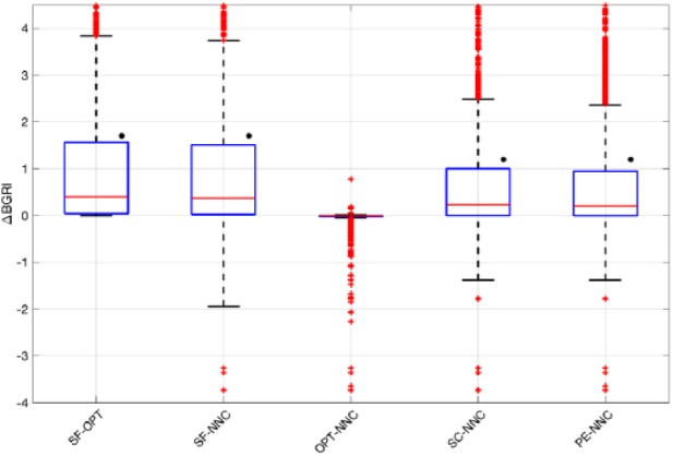
Boxplot representation of the distribution of ΔBGRI obtained comparing (a) SF versus OPT, SF versus NNC, OPT versus NNC, SC versus NNC, and PE versus NNC. Red horizontal lines represent median, boxes mark interquartile ranges, dashed lines are the whiskers, red crosses indicate outliers. Black dots indicate statistical significant between-distributions differences.

Table 1.

Median [Interquartile Range] Results of ΔBGRI (First Row) Obtained Comparing SF Versus OPT, SF Versus NNC, OPT Versus NNC, SC Versus NNC and PE Versus NNC and P Values Obtained Using the Dunn’s Post Hoc Test (Second Row).

	SF-OPT	SF-NNC	OPT-NNC	SC-NNC	PE-NNC
ΔBGRI	0.40 [0.04, 1.56]	0.37 [0.02, 1.51]	0 [–0.02, 0.01]	0.23 [0.01, 0.99]	0.20 [0.01, 0.95]
P value	<.001	<.001	.30	<.001	<.001

Focusing on SF versus NNC, as for SF versus OPT, the obtained results are better in NNC (see Table 1). Notably, the median ΔBGRI and interquartile range is almost the same as in SF versus OPT, meaning that the NNC estimates the optimal target values with good precision. As further proof of the capability of the NNC in estimating the optimal correction values and improving the glycemic outcomes, in Figure 3 we report the distribution of the difference between BGRI in OPT and NNC. No statistically significant difference between the two distributions is found (median difference equal to 0, P = .30). However, Figure 3 points out that, in several scenarios, the NNC error is relevant and, compared to SF, lead to worse BGRI values. In particular, BG control worsens when using NNC to estimate $f(•)$ due to the error the model makes in approximating OPT. This shortcoming represents a limit of the NNC and future work will be performed to properly investigate how to deal with this drawback to guarantee safety and effectiveness in all conditions.

Figure 3 shows the ΔBGRI distribution and median/interquartile results obtained comparing the NNC with SC and PE. Numerical values (median and interquartile range) are reported in the last two columns of Table 1. Overall, according to Figure 3, NNC introduces a small but statistical significant improvement (P < .001) equal to 0.23 and 0.20 if compared with SC and PE, respectively (see Table 1). However, as above, boxplots show that, in several scenarios, NNC lead to worse glycemic outcomes due to the error in the estimate of the optimal $f(•)$ value.

Remark

The effectiveness of the optimal correction $Y_{pm}$ to be applied to the SF is, not surprisingly, related to the structure of the SF itself. Indeed, an accurate analysis of the results of our simulations showed that building a tool able to correct optimally SF seems possible only if, during the training phase, all the possible physiological classes/typologies of the patients at hand are available. While this highlights a restriction of the domain of validity of the NNC presented in this paper, it also suggests that limitations in predicting the optimal correction $Y_{pm}$ are intrinsically related to the strict constraints related to the original structure of SF. Indeed, we found that there is no correlation between $Y_{pm}$ and the actual insulin bolus amount. To better illustrate the point, let us consider two patients having the same meal conditions, that is, same G_C, CHO and IOB, whose optimal insulin boluses are both 0. Since, in general, two patients have different therapy parameters, that is, G_T, CR and CF, this will result in different optimal $Y_{pm}$values. This consideration suggests that correcting SF by a fixed values as defined by $f_{SC}\left(ROC\right)$ and $f_{PE}\left(ROC\right)$ can be, in general, suboptimal.

Discussion and Conclusion

Use of CGM devices in T1D management opened new algorithmic challenges.²⁸ In particular, FDA approval of nonadjunctive use of CGM increased the interest toward methods to “correct” SF of BC to take into account the information on the glucose ROC. Both intuition and evidence provided by the in silico studies²¹ suggest that the optimal modulation of insulin bolus is strongly related to preprandial conditions and individual parameters of the patient.

In this paper, we proposed a new NN-based methodology to personalize insulin bolus calculation exploiting G_C, ROC, IOB, CR, CF, Ib, G_T, BW, V_C, and CHO. An in silico study performed in 100 virtual subjects in noise-free conditions, showed that, in terms of glycemic outcomes measured as BGRI over 24 hours, the new method outperforms the literature approaches SF, SC, and PE, and is close to the optimum determined by exhaustive search. Although, quantitatively improvements might seem minor, these preliminary results encourage further investigations on machine learning-based methodologies to provide patients with decision support tools able to ease their daily insulin therapy routine. With regard to this aspect, it is important to stress that, in the present investigation of tools to predict the optimal correction of SF, we limited ourselves to evaluating NNs. Of course, other nonlinear machine learning techniques (eg, kernel support vector machines or regression trees) could be considered for the scope as well. Implementation of alternative methods will be matter of future investigations, together with a comprehensive analysis of the relative performance of the so-obtained calculators. In particular, a margin of improvement emerged from the Remark 1 reported in the Results lies in relaxing the strict constraints related to the original structure of SF by devising new methods to compute directly the optimal insulin bolus. Work presently underway at our lab concerns the development of machine learning techniques capable to “learn” new optimal dosing rules using the information provided by CGM devices.

To conclude, future work will also involve testing the NNC on more challenging scenarios by means of the T1D patient decision simulator of Vettoretti et al,²⁹ which expands the model employed in the UVA/Padova T1D Simulator by new modules describing error of glucose monitoring sensors (both self-monitoring of blood glucose²⁹ and CGM³⁰) and patient behavior. In addition, another interesting aspect would be furtherly exploring both the NNC structure by reducing the number of nodes in the middle layer and introducing fuzzification as a way to accommodate person-to-person variation and expanding the feature set we used to train NNC. For example, it will be worth adding as inputs also a preprandial window of CGM values to exploit fully the information on BG dynamic provided by CGM devices. Finally, it would be also interesting to investigate how the NNC performance is influenced by the variability of CGM sensor accuracy, for example, observed for different days of sensor wear or different number of sensor’s calibrations per day.^31-34

References

- 1. American Diabetes Association. Classification and diagnosis of diabetes. Diabetes Care. 2017;40(suppl 1):s11-s24. [DOI] [PubMed] [Google Scholar]
- 2. Schmidt S, Norgaard K. Bolus calculators. J Diabetes Sci Technol. 2014;8:1035-1041. [DOI] [PMC free article] [PubMed] [Google Scholar]
- 3. Gross TM, Kayne D, King A, Rother C, Juth S. A bolus calculator is an effective means of controlling postprandial glycemia in patients on insulin pump therapy. Diabetes Technol Ther. 2003;10:365-369. [DOI] [PubMed] [Google Scholar]
- 4. Klonoff DC. The current status of bolus calculator decision-support software. J Diabetes Sci Technol. 2012;6:990-994. [DOI] [PMC free article] [PubMed] [Google Scholar]
- 5. Davidson PC, Hebblewhite HR, Steed RD, Bode BW. Analysis of guidelines for basal-bolus insulin dosing: basal insulin, correction factor and carbohydrate-to-insulin ratio. Endocr Prat. 2008;14:1095-1101. [DOI] [PubMed] [Google Scholar]
- 6. Reiterer F, Kirchsteiger H, Assalone A, Freckmann G, Del Re L. Performance assessment of estimation methods for CIR/ISF in bolus calculators. In: Proceedings of the 9th IFAC Symposium on Biological and Medical Systems (BMS 2015) Berlin, Germany: IFAC; 2015:231-236. [Google Scholar]
- 7. Edelman SV. Regulation catches up to reality non-adjunctive use of continuous glucose monitoring data. J Diabetes Sci Technol. 2017;1:160-164. [DOI] [PMC free article] [PubMed] [Google Scholar]
- 8. US Food and Drug Administration. Dexcom G5 mobile continuous glucose monitoring system. Available at: https://www.accessdata.fda.gov/cdrh_docs/pdf12/P120005S041a.pdf. Accessed November 15, 2017.
- 9. Cappon G, Acciaroli G, Vettoretti M, Facchinetti A, Sparacino G. Wearable continuous glucose monitoring sensors: a revolution in diabetes treatment [published online ahead of print September 5, 2017]. Electronics. doi: 10.3390/electronics6030065. [DOI] [Google Scholar]
- 10. Scheiner G. Practical CGM: Improving Patient Outcomes Through Continuous Glucose Monitoring. Alexandria, WV: American Diabetes Association; 2015. [Google Scholar]
- 11. Pettus J, Edelman SV. Recommendations for using real-time continuous glucose monitoring (rtCGM) data for insulin adjustments in type 1 diabetes. J Diabetes Sci Technol. 2017;11:138-147. [DOI] [PMC free article] [PubMed] [Google Scholar]
- 12. Cobelli C, Dalla Man C, Sparacino G, Magni L, De Nicolao G, Kovatchev BP. Diabetes: models, signals, and control. IEEE Rev Biomed Eng. 2009;2:54-96. [DOI] [PMC free article] [PubMed] [Google Scholar]
- 13. Kovatchev B, Breton M, Dalla Man C, Cobelli C. In silico preclinical trials: a proof of concept in closed-loop control of type 1 diabetes. J Diabetes Sci Technol. 2009;3:44-55. [DOI] [PMC free article] [PubMed] [Google Scholar]
- 14. Hovorka R, Canonico V, Chassin LJ, et al. Nonlinear model predictive control of glucose concentration in subjects with type 1 diabetes. Physiol Meas. 2004;25:905-920. [DOI] [PubMed] [Google Scholar]
- 15. Wilinska EM, Chassin LJ, Acerini CL, Allen JM, Dunger DB, Hovorka R. Simulation environment to evaluate closed-loop insulin delivery systems in type 1 diabetes. J Diabetes Sci Technol. 2010;4:132-144. [DOI] [PMC free article] [PubMed] [Google Scholar]
- 16. Kanderian SS, Weinzimer S, Voskanyan G, Steil GM. Identification of intraday metabolic profiles during closed loop glucose control in individuals with type 1 diabetes. J Diabetes Sci Technol. 2009;3:1047-1057. [DOI] [PMC free article] [PubMed] [Google Scholar]
- 17. Patek SD, Lv D, Ortiz EA, et al. Empirical representation of blood glucose in a compartmental model. In: Kirchsteiger H, Jørgensen JB, Renard E, del Re L. eds. Prediction Methods for Blood Glucose Concentration. Cham, Switzerland: Springer; 2016:183-209. [Google Scholar]
- 18. Vettoretti M, Facchinetti A, Sparacino G, Cobelli C. Predicting insulin treatment scenarios with the net effect method: domain of validity. Diabetes Technol Ther. 2016;18:694-704. [DOI] [PubMed] [Google Scholar]
- 19. Vettoretti M, Facchinetti A, Sparacino G, Cobelli C. Type 1 diabetes patient decision simulator for in silico testing safety and effectiveness of insulin treatments [published online ahead of print August 29, 2017]. IEEE Trans Biomed Eng. doi: 10.1109/TBME.2017.2746340. [DOI] [PubMed] [Google Scholar]
- 20. Reiterer F, Reiterer M, Del Re L. Hybrid in silico evaluation approach for assessing insulin dosing strategies. In: Proceedings of the 20th IFAC World Congress Toulouse, France: IFAC; 2017:2051-2057. [Google Scholar]
- 21. Marturano F, Cappon G, Vettoretti M, Facchinetti A, Sparacino G. In silico assessment of literature methods to adjust insulin bolus dose according to CGM trend. In: 17th Annual Diabetes Technology Meeting (DTM), Bethesda, MD: DTM; 2017. [Google Scholar]
- 22. Dalla Man C, Micheletto F, Lv D, Breton M, Kovatchev B, Cobelli C. The UVa/Padova type 1 diabetes simulator: new features. J Diabetes Sci Technol. 2014;8:26-34. [DOI] [PMC free article] [PubMed] [Google Scholar]
- 23. Fabris C, Patek SD, Breton MD. Are risk indices derived from CGM interchangeable with SMBG-based indices? J Diabetes Sci Technol. 2016;10:50-59. [DOI] [PMC free article] [PubMed] [Google Scholar]
- 24. Srivastava N, Hinton G, Krizhevsky A, Sutskever I, Salakhutdinov R. Dropout: a simple way to prevent neural networks from overfitting. J Machine Learning Res. 2014;15:1929-1958. [Google Scholar]
- 25. Visentin R, Dalla Man C, Kudva YC, Basu A, Cobelli C. Circadian variability of insulin sensitivity: physiological input for in silico artificial pancreas. Diabetes Technol Ther. 2014;17:1-7. [DOI] [PMC free article] [PubMed] [Google Scholar]
- 26. Hinton G, Srivastava N, Swersky K. Overview of mini-batch gradient descent. Neural Network for Machine Learning, Coursera Course. Available at: http://www.cs.toronto.edu/~tijmen/csc321/slides/lecture_slides_lec6.pdf. Accessed November 15, 2017.
- 27. Bergstra J, Bardenet R, Bengio Y, Kégl B. Algorithms for hyper-parameter optimization. In: Advances in Neural Information Processing Systems 24 (NIPS 2011). Granada, Spain: NIPS; 2011:2546-2554. [Google Scholar]
- 28. Facchinetti A. Continuous glucose monitoring sensors: past, present and future algorithmic challenges. Sensors. 2016;16:E2093. [DOI] [PMC free article] [PubMed] [Google Scholar]
- 29. Vettoretti M, Facchinetti A, Sparacino G, Cobelli C. A model of self-monitoring blood glucose measurement error. J Diabetes Sci Technol. 2017;11:724-735. [DOI] [PMC free article] [PubMed] [Google Scholar]
- 30. Facchinetti A, Del Favero S, Sparacino G, Cobelli C. Model of glucose sensor error components: identification and assessment for new Dexcom G4 generation devices. Med Biol Eng Comput. 2015;53:1259-1269. [DOI] [PubMed] [Google Scholar]
- 31. Bailey TS, Chang A, Christiansen M. Clinical accuracy of a continuous glucose monitoring system with an advanced algorithm. J Diabetes Sci Technol. 2014;9:209-214. [DOI] [PMC free article] [PubMed] [Google Scholar]
- 32. Bailey TS, Ahmann A, Brazg R, et al. Accuracy and acceptability of the 6-day Enlite continuous subcutaneous glucose sensor. Diabetes Technol Ther. 2014;16:277-283. [DOI] [PubMed] [Google Scholar]
- 33. Acciaroli G, Vettoretti M, Facchinetti A, Sparacino G, Cobelli C. From two to one per day calibration of Dexcom G4 Platinum by a time-varying day-specific Bayesian prior. Diabetes Technol Ther. 2016;18:472-479. [DOI] [PubMed] [Google Scholar]
- 34. Acciaroli G, Vettoretti M, Facchinetti A, Sparacino G, Cobelli C. Reduction of blood glucose measurements to calibrate subcutaneous glucose sensors: a Bayesian multi-day framework [published online ahead of print May 23, 2017]. IEEE Trans Biomed Eng. doi: 10.1109/TBME.2017.2706974. [DOI] [PubMed] [Google Scholar]