q-Space Upsampling Using x-q Space Regularization

Abstract

Acquisition time in diffusion MRI increases with the number of diffusion-weighted images that need to be acquired. Particularly in clinical settings, scan time is limited and only a sparse coverage of the vast q-space is possible. In this paper, we show how non-local self-similar information in the x-q space of diffusion MRI data can be harnessed for q-space upsampling. More specifically, we establish the relationships between signal measurements in x-q space using a patch matching mechanism that caters to unstructured data. We then encode these relationships in a graph and use it to regularize an inverse problem associated with recovering a high q-space resolution dataset from its low-resolution counterpart. Experimental results indicate that the high-resolution datasets reconstructed using the proposed method exhibit greater quality, both quantitatively and qualitatively, than those obtained using conventional methods, such as interpolation using spherical radial basis functions (SRBFs).

1 Introduction

Diffusion magnetic resonance imaging (MRI) offers insight into the neural pathways of the human brain by probing the diffusion of water molecules in multiple directions and scales. A diffusion MRI protocol normally acquires multiple diffusion-weighted images, each corresponding to a wavevector q in q-space. The vector q can be separated into a scalar wavenumber |q| and a diffusion encoding direction q̂ = q/|q|. The effects of both diffusion time, t, and wavenumber are summarized using a quantity called b-value, which is defined as b = t|q|². Depending on the application, the q-space can be covered using different sampling schemes, such as Cartesian sampling as in diffusion spectrum imaging (DSI) and multi-shell sampling with multiple distinct b-values.

In general, the number of diffusion-weighted images that need to be acquired increases with the complexity of the diffusion model one is interested in fitting to the data. For example, the diffusion tensor model requires a minimum of only 6 diffusion-weighted images and one without diffusion weighting. However, for a more realistic account of the white matter (WM) neuronal architecture, such as fiber crossings and intra-/extra-cellular compartments, more sophisticated models are needed. To reliably estimate the parameters of these models, a greater number of diffusion-weighted images are needed. This requirement is difficult to meet when time allotted for acquisition is limited, especially in clinical settings.

One way to increasing q-space resolution without additional acquisition time is by post-acquisition upsampling. Currently, only a few methods have been developed for this purpose. The most commonly used method is interpolation using spherical radial basis functions (SRBFs) [1]. A more recent approach proposed by Yap et al. [2] utilizes wavelet frames defined on graphs for sparsity-enforcing q-space upsampling. These methods, however, only employ q-space measurements for upsampling and neglect signal correlation across voxels in x-space.

In this paper, we introduce a method for q-space upsampling by leveraging non-local self-similar information in the x-q space. Our consideration of the joint x-q space allows information from curved WM structures to be used more effectively for upsampling. The contributions of the current work are as follows: (1) Upsampling based directly on the diffusion-weighted images. No model is assumed, other than non-local smoothness. (2) Non-local relationships of q-space samples are learned over both x space and q space to help regularize the otherwise ill-posed inverse problem involved in recovering the high q-space resolution data from the low resolution counterparts. (3) Our method can effectively use information from curved white matter structures because joint x-q space patch matching is tolerant of angular differences. (4) Our results indicate that the proposed method can help compensate for insufficient sampling in q-space due to time constraints.

2 Approach

Our approach first establishes the relationships of the signal samples in x-q space using robust neighborhood matching. These relationships are then used to regularize the inverse problem that needs to be solved to recover the high resolution data.

2.1 Establishing Relationships of Signals in x-q Space

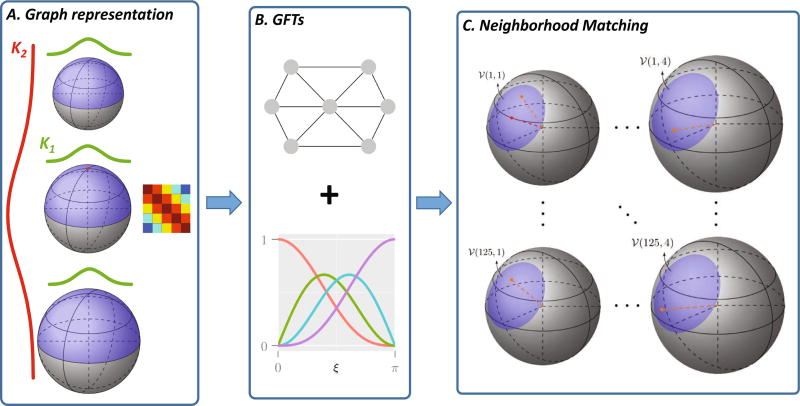
For each pair of signal measurements in x-q space, a similarity weight is assigned based on robust patch matching using a method similar to [3,4]. Conventional x-space neighborhood matching methods, such as non-local means, has demonstrated remarkable performance in locating recurrent image patterns. We extend this to x-q space so that neighborhood matching can be performed effectively for curved white matter structures. We (1) Generate a rotation invariant feature vector for each sampling point in x-q space and (2) Perform neighborhood matching for each pair of points in x-q space. See Fig. 1 for an overview.

Fig. 1. Overview.

(A) Representing the sampling domain using a graph with affinity matrix determined by kernel K₁ across directions and kernel K₂ across diffusion weightings. (B) Computation of rotation-invariant features using GFTs. (C) Neighborhood matching.

Rotation-invariant features

We use graph framelet transforms (GFTs) [2] to generate a rotation-invariant and multi-scale feature vector for each sampling point in x-q space. GFTs can be used to generate a wavelet representation for data that are not necessarily residing on a Cartesian grid. In our case, the data in q-space is unstructured and may not distribute uniformly. GTFs involve representing the sampling domain in q-space as a graph, computing the eigen-spectrum based on the graph Laplacian, and then performing multiresolution analysis based on the spectrum. The interested reader is referred to [2] for more details.

Neighborhood matching in x-q space

Figure 1(C) illustrates how neighborhood matching is performed in x-q space. Neighborhood matching is performed based on a reference point marked in red within a search neighborhood 𝒱(1, 1) marked in blue. In the specific example given in Fig. 1(C), this is done across 4 q-shells (columns) and in a x-space of 2-voxel radius (rows), i.e., a 125 voxel neighborhood. Example candidate points are marked in orange. A similarity weight is assigned to each candidate point. For more details, please refer to [3,4].

2.2 q-Space Upsampling

We use the x-q space data relationships determined in the previous section to guide data upsampling in the q space. For simplicity, we represent the low angular resolution (LAR) data using vector y and the high angular resolution (HAR) that we need to estimate using vector x. The objective function of our problem is as follows:

$${\epsilon }^2(\mathbf{x})=\frac{\lambda }{2}{\Vert \mathbf{\text{Ax}}-\mathbf{y}\Vert }_2^2+\frac{1}{4}\sum _{(i,k)\in \mathrm{\Omega }}\sum _{(j,l)\in 𝒱(i,k)}w[i,k;j,l]{\Vert {\mathbf{R}}_{i,k}\mathbf{x}-{\mathbf{R}}_{j,l}\mathbf{x}\Vert }_2^2,$$ (1)

where A is a q-space downsampling operator, w[i, k; j, l] is a weight determined by neighborhood matching, R_i,k is an operator that extracts the diffusion signal associated with an x-space index i and a q-space index k. The penalty function consists of a data fidelity term and a regularization term based on x-q space neighborhood matching. To minimize (1), we compute the derivative and equate it to zero:

$$0=\frac{d{\epsilon }^2(\mathbf{x})}{d\mathbf{x}}=\lambda {\mathbf{A}}^{\top }(\mathbf{\text{Ax}}-\mathbf{y})+\frac{1}{2}\sum _{(i,k)\in \mathrm{\Omega }}\sum _{(j,l)\in 𝒱(i,k)}w[i,k;j,l]\times {({\mathbf{R}}_{i,k}-{\mathbf{R}}_{j,l})}^{\top }({\mathbf{R}}_{i,k}-{\mathbf{R}}_{j,l})\mathbf{x}.$$ (2)

Using the facts that the neighborhood is symmetric (i.e., if (j, l) ∈ 𝒱(i, k), then (i, k) ∈ 𝒱(j, l)) and the weights are symmetric (i.e., w[i, k; j, l] = w[j, l; i, k]), the equation above can be simplified as [5]

$$0=\lambda {\mathbf{A}}^{\top }(\mathbf{\text{Ax}}-\mathbf{y})+\sum _{(i,k)\in \mathrm{\Omega }}\sum _{(j,l)\in 𝒱(i,k)}w[i,k;j,l]{\mathbf{R}}_{i,k}^{\top }{\mathbf{R}}_{i,k}\mathbf{x}-\sum _{(i,k)\in \mathrm{\Omega }}\sum _{(j,l)\in 𝒱(i,k)}w[i,k;j,l]{\mathbf{R}}_{i,k}^{\top }{\mathbf{R}}_{j,l}\mathbf{x}.$$ (3)

Equation (3) can be solved directly but involves the inversion of a very large matrix. To avoid this, we choose instead to use fixed-point iteration [5] to solve the problem. If we let xⁿ be the solution at iteration n, the following can be proven to be convergent [5]:

$$0=\lambda {\mathbf{A}}^{\top }({\mathbf{\text{Ax}}}^n-\mathbf{y})+\sum _{(i,k)\in \mathrm{\Omega }}\sum _{(j,l)\in 𝒱(i,k)}w[i,k;j,l]{\mathbf{R}}_{i,k}^{\top }{\mathbf{R}}_{i,k}{\mathbf{x}}^n-\sum _{(i,k)\in \mathrm{\Omega }}\sum _{(j,l)\in 𝒱(i,k)}w[i,k;j,l]{\mathbf{R}}_{i,k}^{\top }{\mathbf{R}}_{j,l}{\mathbf{x}}^{n-1}.$$ (4)

The solution x can be obtained iteratively using

$${\mathbf{x}}^n={(\lambda {\mathbf{A}}^{\top }\mathbf{A}+\sum _{(i,k)\in \mathrm{\Omega }}\sum _{(j,l)\in 𝒱(i,k)}w[i,k;j,l]{\mathbf{R}}_{i,k}^{\top }{\mathbf{R}}_{i,k})}^{-1}\times (\lambda {\mathbf{A}}^{\top }\mathbf{y}+\sum _{(j,l)\in \mathrm{\Omega }}\sum _{(i,k)\in 𝒩(k,l)}w[i,k;j,l]{\mathbf{R}}_{i,k}^{\top }{\mathbf{R}}_{j,l}{\mathbf{x}}^{n-1}).$$ (5)

The matrix inversion in (5) involves a block diagonal matrix and can therefore be done effectively.

2.3 Implementation Issues

Initialization

The data are transformed so that the noise is Gaussian distributed as described in [6]. The algorithm is then initialized using an upsampled version of y, which is obtained via interpolation using SRBFs.

Neighborhood matching

Neighborhood matching is performed based on the upsampled version of y. The resulting weights remain unchanged until a solution x is obtained. In principle, we can use x to re-estimate the weights and rerun the algorithm to obtain a refined solution. However, our experimental results indicate that the benefit of doing so is minimal. Therefore, we will only show results without weight re-estimation.

Stopping criterion

We stop the algorithm when the mean absolute difference (MAD) between the outcomes of two iterations, i.e., xⁿ⁻¹ and xⁿ, is less than a constant tol. We define tol = βσ_G, where σ_G is the standard derivation of the Gaussian noise and β is a constant.

3 Experiments

We evaluated the proposed q-space upsampling algorithm using both synthetic and real data. Through grid search, we found that λ = 10 and β = 10⁻⁴ give the best results. We used the upsampled data obtained using SRBF interpolation as a comparison baseline. This was also used for the initialization of our algorithm. The peak-to-signal ratio (PSNR) was used as the metric for quantitative evaluation.

3.1 Synthetic Data

A set of synthetic data was generated using phantomαs [7]. Two sets of diffusion gradient directions were utilized to simulate the high (H) and low (L) angular resolution (AR) diffusion MRI data. The LAR gradients were generated by dividing the faces of an icosahedron three times and discarding antipodal symmetric directions, giving us a total of 81 directions uniformly distributed on a hemisphere. Based on the same strategy, we generated the HAR gradient directions by dividing the faces of the icosahedron four times to obtain 321 directions. Data for 3 shells, b = 1000, 2000, 3000 s/mm², were generated. Finally, we added three levels of 32-channel noncentral chi noise to the LAR data, with per-channel Gaussian standard deviation σ_G = 40, 80 and 120 corresponding to 2%, 4% and 6% of the mean signal value of all diffusion-weighted images.

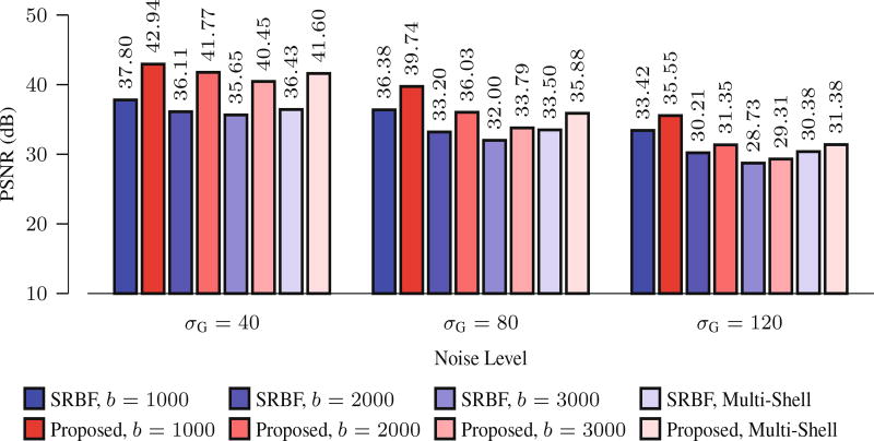
Using the noise-free HAR data as ground truth, we evaluated the quality of the upsampled data using PSNR. The results, shown in Fig. 2, indicate that the proposed method outperforms SRBF interpolation for all noise levels and b-values. For the single-shell case, the largest improvement, 5.65 dB, was obtained when σ_G = 40 and b = 2000 s/mm². For the multi-shell case, the largest improvement, 5.18 dB, was obtained when σ_G = 40.

Fig. 2. PSNR Comparison.

Quantitative evaluation using synthetic data.

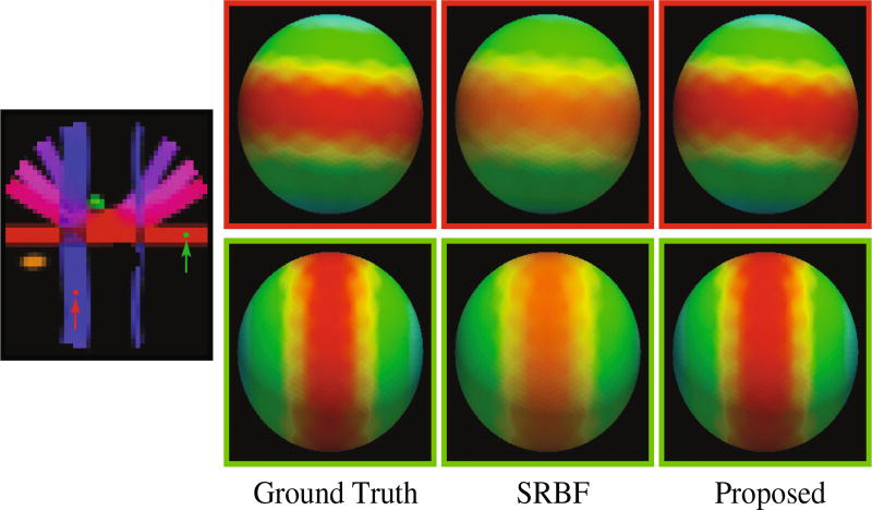
For a more direct visualization of the improvements given by the proposed method, we rendered the signal values on a sphere. The results, shown in Fig. 3, indicate that the proposed method gives values that are closer to the ground truth. In contrast, the results given by SRBF interpolation are over-smoothed and are not as close to the ground truth.

Fig. 3. Diffusion Signal Profiles.

The diffusion signals are rendered on a sphere for visual comparison. The colored FA image is shown on the far left for reference.

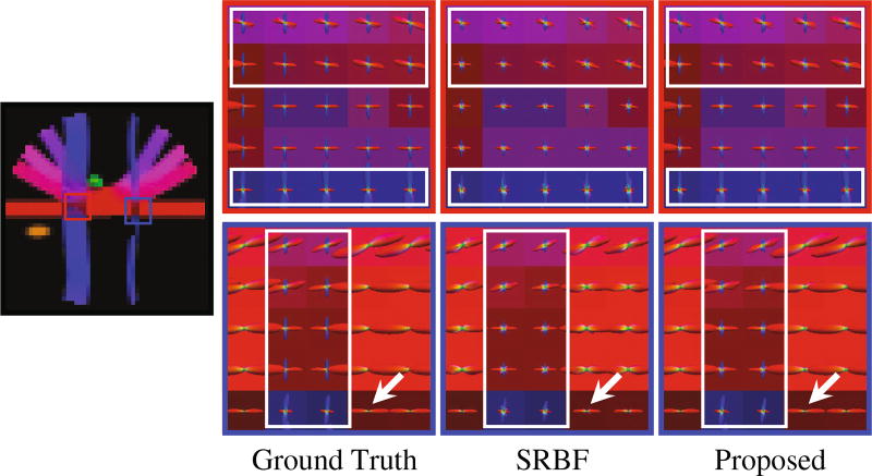
Accurate ODF estimation relies on sufficient angular samples. The ODFs, shown in Fig. 4, indicate that our method gives clean and coherent ODFs that are close to the ground truth. In contrast, spurious peaks are introduced by SRBF interpolation.

Fig. 4. ODFs.

Fiber ODF comparison using synthetic data.

3.2 Real Data

We used 10 diffusion MRI datasets randomly selected from the Human Connectome Project (HCP) [8]. The imaging protocol is as follows: 145 × 174 imaging matrix, 1.25 × 1.25 × 1.25 mm³ resolution, TE = 89 ms, TR = 5500 ms, 145 slices, 90 non-colinear gradient directions in each shell. We uniformly selected 45 gradient directions per shell to generate the LAR data for evaluation.

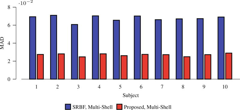
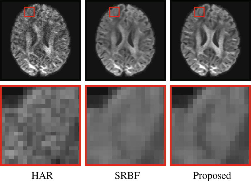
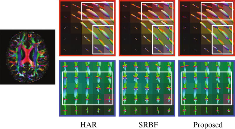
Using the original HAR data directly as the ground truth for quantitative evaluation will introduce bias owing to noise. To reduce the effect of noise, we fitted the diffusion tensor model and used fractional anisotropy (FA) for evaluation. Figure 5 shows the mean absolute difference (MAD) between the FA values given by the upsampled data and the ground truth HAR data. For all 10 datasets, our method outperforms SRBF interpolation, with a largest MAD reduction of 0.0429. The top row of Fig. 6 indicates that the proposed method results in better structural contrast. Close-up views, shown in the bottom row of Fig. 6, further confirm that subtle structures are preserved. Figure 7 indicates that our method gives clean and coherent ODFs.

Fig. 5. MAD Comparison.

Quantitative evaluation using real data.

Fig. 6. Diffusion-Weighted Images.

Comparison of upsampled diffusion-weighted images with the original HAR data.

Fig. 7. ODFs.

Comparison of fiber ODFs using real data.

4 Conclusion

In this paper, we have proposed a method for q-space upsampling of diffusion MRI data. The data relationships in x-q is first established using a robust x-q space patch matching mechanism. These relationships are then used to regularize the inverse problem associated with recovering the high angular resolution data. Experiments on both synthetic and real data demonstrated the effectiveness of proposed method. In the future, we will extend the proposed framework to upsampling in both x-space and q-space.

References

- 1.Tuch DS. Q-ball imaging. Magn. Reson. Med. 2004;52:1358–1372. doi: 10.1002/mrm.20279. [DOI] [PubMed] [Google Scholar]
- 2.Yap PT, Dong B, Zhang Y, Shen D. International Conference on Medical Image Computing and Computer-Assisted Intervention. Springer; New York: 2016. Tight graph framelets for sparse diffusion MRI q-space representation; pp. 561–569. [DOI] [PMC free article] [PubMed] [Google Scholar]
- 3.Chen G, Wu Y, Shen D, Yap PT. XQ-NLM: denoising diffusion MRI data via x-q space non-local patch matching. In: Ourselin S, Joskowicz L, Sabuncu MR, Unal G, Wells W, editors. MICCAI 2016. LNCS. Vol. 9902. Springer, Cham; 2016. pp. 587–595. [DOI] [PMC free article] [PubMed] [Google Scholar]
- 4.Chen G, Dong B, Zhang Y, Shen D, Yap PT. Denoising of diffusion MRI data using manifold neighborhood matching. OHBM Annual Meeting. 2017 [Google Scholar]
- 5.Protter M, Elad M, Takeda H, Milanfar P. Generalizing the nonlocal-means to super-resolution reconstruction. IEEE Trans. Image Proc. 2009;18(1):36–51. doi: 10.1109/TIP.2008.2008067. [DOI] [PubMed] [Google Scholar]
- 6.Chen G, Shen D, Yap PT. Non-central Chi to Gaussian transformation of diffusion MRI signals improves estimation of fiber ODFs. ISMRM. 2017 [Google Scholar]
- 7.Caruyer E, Daducci A, Descoteaux M, Houde JC, Thiran JP, Verma R. Phantomas: a flexible software library to simulate diffusion MR phantoms. ISMRM. 2014 [Google Scholar]
- 8.Essen DCV, Smith SM, Barch DM, Behrens TE, Yacoub E, Ugurbil K. The WU-Minn human connectome project: An overview. NeuroImage. 2013;80:62–79. doi: 10.1016/j.neuroimage.2013.05.041. [DOI] [PMC free article] [PubMed] [Google Scholar]