Distinct timescales of population coding across cortex

Abstract

The cortex represents information across widely varying timescales^1–5. For instance, sensory cortex encodes stimuli that fluctuate over few tens of milliseconds^6,7, whereas in association cortex behavioral choices can require the maintenance of information over seconds^8,9. However, it remains poorly understood if diverse timescales result mostly from features intrinsic to individual neurons or from neuronal population activity. This question is unanswered because the timescales of coding in populations of neurons have not been studied extensively, and population codes have not been compared systematically across cortical regions. Here we discovered that population codes can be essential to achieve long coding timescales. Furthermore, we found that the properties of population codes differ between sensory and association cortices. We compared coding for sensory stimuli and behavioral choices in auditory cortex (AC) and posterior parietal cortex (PPC) as mice performed a sound localization task. Auditory stimulus information was stronger in AC than in PPC, and both regions contained choice information. Although AC and PPC coded information by tiling in time neurons that were transiently informative for ~200 milliseconds, the areas had major differences in functional coupling between neurons, measured as activity correlations that could not be explained by task events. Coupling among PPC neurons was strong and extended over long time lags, whereas coupling among AC neurons was weak and short-lived. Stronger coupling in PPC led to a population code with long timescales and a representation of choice that remained consistent for approximately one second. In contrast, AC had a code with rapid fluctuations in stimulus and choice information over hundreds of milliseconds. Our results reveal that population codes differ across cortex and that coupling is a variable property of cortical populations that affects the timescale of information coding and the accuracy of behavior.

The goal of this work was to compare coding across cortical regions for two key features of behavioral tasks: stimulus and choice. We developed a sound localization task in which mice reported perceptual decisions by navigating through a visual virtual reality T-maze¹⁰ (Fig. 1a). As mice ran down the T-stem, a sound cue was played from one of eight possible locations in head-centered, real-world coordinates. Mice reported whether the sound originated from their left or right by turning in that direction at the T-intersection (Fig. 1b–c).

Figure 1. Imaging AC and PPC responses during a sound localization task.

a, Schematic of experimental set-up with VR screenshots for the beginning of the trial and T-intersection. b, Schematic of the task. Left/Right sound category (speaker symbols), indicated the rewarded side of the maze (checkmark). c, Behavioral performance. Each line is the average across sessions for a single mouse. n = 5 mice. d–e, z-scored, trial-averaged activity of all AC and PPC neurons, sorted by time of peak mean activity. f, Average responses of example AC and PPC neurons on correct (black) and error (gray) trials.

We focused on AC because it is necessary for sound localization tasks¹¹ and on PPC because it is involved in spatial auditory processing¹², receives inputs from AC, is a multisensory-motor interface^{8–10,13–17}, and is essential for virtual-navigation tasks¹⁰. In each mouse, we imaged the activity of ~50 neurons simultaneously from AC and PPC on separate days. In both regions, neurons were transiently active at different time points, resulting in a population that tiled the trial (Fig. 1d–e). Activity in some AC neurons was selective for stimulus location; however, as a population, AC activity was heterogeneous and complex (Fig. 1d,f; Extended Data Fig. 1; Supplementary Information). In PPC, a substantial fraction of neurons had different activity on trials with opposite behavioral choices^{8–10,15–18} (Fig. 1f).

The heterogeneity of activity patterns suggested that, in addition to stimulus and choice, multiple task-related variables, such as visual inputs, reward delivery, and the mouse’s running, might affect neuronal responses. To take these variables into account and to help isolate signals related to stimulus and choice, we developed an encoding model (generalized linear model - GLM). This model incorporated all measured task-related variables as predictors of each neuron’s activity^19,20 (Fig. 2a, Extended Data Fig. 2a–d). The model reliably predicted the time course and selectivity of single neuron activity in AC and PPC (Fig. 2b–c; Extended Data Fig. 2g).

Figure 2. Encoding and decoding stimulus and choice information in AC and PPC.

a, The encoding model (GLM) was fit to each neuron’s activity using task predictors (“uncoupled model”) or task predictors and activity of other neurons (coupling predictors, “coupled model”). To decode stimuli or choices (indicated as ν), the posterior probability of each stimulus or choice was computed, based on the current time point only (“instantaneous decoder”), or all previous time points in the trial (“cumulative decoder”). The decoder could use either all neurons (population decoder) or individual neurons (single-neuron decoder). b–c, Example trial-averaged responses (left column) and model predictions (right column) in correct (black) and error (gray) trials. d–e, Cumulative stimulus category and choice information decoded in AC (red) and PPC (blue) populations. Shading indicates mean ± sem across datasets. n = 7 datasets for AC and PPC. f–h, Max-normalized instantaneous information about stimulus category and choice for AC and PPC cells with at least 0.06 bits of information at any point in the trial (fraction of all cells: AC: stimulus, 20.2 ± 5.4%; choice, 15.9 ± 3.2%; PPC: stimulus, 3.1 ± 1.3%; choice, 19.3 ± 4.6%). Neurons were sorted by the times of their maximum information. i–j, Information about stimulus category and choice averaged across all AC (red) and PPC (blue) cells, calculated as a two-sided decay (forward and backward in time) around the information peak of each cell. Shading indicates mean ± sem across cells with at least 0.06 bits of information. k, Decay time constant of single-cell information from exponential fits to information time courses in (i–j). Error bars: 95% confidence intervals (Methods). *** indicates p < 0.001, z-test.

To determine whether stimulus and choice information were present in AC and PPC, we decoded the most likely stimulus category (left or right location) or choice (left or right turn) from neuronal activity by using Bayes’ rule to invert the prediction of the encoding model (Fig. 2a). Because stimulus locations and choices were related to one another by task design (e.g. left stimuli required a left turn for reward), we decoupled these features and isolated information purely related to stimulus from information purely related to choice by selecting equal numbers of right and left choice trials for analysis in each stimulus condition (thus the same number of correct and error trials). Decoding performance was calculated as the mutual information between the decoded and actual stimulus category or choice.

Pure information about the stimulus category was present in AC activity but was weak in PPC (Fig. 2d). Information purely about the choice was present in both AC and PPC populations (Fig. 2e). Although the mouse’s running patterns that triggered turns in the virtual environment necessarily covaried with the choice at some trial time points, the choice information estimated by our decoding analysis was similar even when fully discounting the effects of running patterns (Extended Data Fig. 3g–i). AC and PPC thus likely contained genuine choice information. Additional analyses that did not decouple stimulus and choice revealed that both regions had a relationship between neuronal tuning for stimulus and choice and contained information at the intersection between stimulus and choice²¹ (Supplementary Information; Extended Data Fig. 3a–f, Extended Data Fig. 4a). The information present in both regions thus appeared to be used for performing the task.

We investigated the codes for stimulus and choice information first by examining activity in single neurons. In AC, we considered both stimulus and choice information, whereas, in PPC, we focused on choice information only because PPC contained little pure stimulus information. Stimulus and choice information were small but significant in individual neurons, on average, and only a minority of neurons had large stimulus or choice information (Extended Data Fig. 4b–j). In both areas, individual neurons were briefly informative, with subsets of largely distinct neurons providing information at different time points in a trial^10,22 (Fig. 2f–k). Single cells in AC and PPC were informative about the choice for ~100 and 300 ms, respectively, and individual AC cells were informative about the stimulus category for ~280 ms (calculated as a two-sided decay around the information peak of each cell; Fig. 2i,k). Therefore, in most individual neurons, information was weak and short-lived relative to the length of trials.

We thus reasoned that population codes may be important in AC and PPC, in particular if long-duration and diverse timescales were present. To examine the structure of functional interactions in population activity^18,23–27, we modified our encoding model to predict a given neuron’s activity based on the past activity of each of the other imaged neurons (“coupling predictors”; activity from up to ~2 s in the past, within defined lag ranges). These coupling predictors were included in a single model along with the task-related predictors described above²⁰ (“task predictors”; Fig. 3a–c). Here “coupling” indicates functional interactions between neurons without necessarily implying a direct causal connection between them. We quantified how strongly a neuron was coupled with other neurons in the local population by computing a “coupling index”: the difference in performance between the models with and without coupling predictors divided by the coupled model performance. Higher coupling indices indicated that other neurons’ activity provided greater improvement in the prediction of a neuron’s moment-to-moment activity patterns beyond what could be modeled with task features alone. Coupling is conceptually similar to “noise” correlation²³, but it discounts, on a trial-by-trial basis, effects arising from shared tuning to measured task events and includes all other simultaneously imaged neurons.

Figure 3. PPC populations were more coupled than AC populations.

a, For a PPC neuron with high coupling index, single trial responses (magenta) and predicted responses from the uncoupled (cyan) and coupled (black) models. b–c, Prediction performance of the coupled and uncoupled models for all AC and PPC neurons (circles). d, Cumulative distribution of the coupling index in AC (red) and PPC (blue) neurons. *** indicates p < 0.001, KS test. e, Coupling index in coupled model variants using as coupling predictors the mean population activity, 3–12 factors extracted from the population activity, or all other simultaneously imaged neurons. *** indicates p < 0.001, rank sum test. f, Mean coupling index in AC (red) and PPC (blue) when coupling predictors were shifted by different temporal lags relative to the predicted neuron’s activity. Error bars indicate mean ± sem. * indicates p < 0.05; ** p < 0.01; *** p < 0.001; rank sum test comparing PPC vs. AC. Only neurons with fraction explained deviance > 0.1 in the coupled model were included in panels d–f (n = 174/329 AC neurons and n = 185/386 PPC neurons).

Strikingly, the activity of PPC neurons had nearly three times more contribution from near-instantaneous coupling than did AC neurons, on average (coupling index: AC, 0.14 ± 0.02; PPC, 0.40 ± 0.02, p < 0.001, KS test; Fig. 3d). Coupling between PPC neurons was present even at lags in activity up to ~1.25 s (p < 0.001, signed-rank test; Fig. 3f). In contrast, AC coupling was weak at all lags (Fig. 3f). This difference in coupling was confirmed by calculating partial Pearson correlations for activity in neuron pairs (Extended Data Fig. 5). AC and PPC therefore had major differences in the structure of population activity, with higher coupling among neurons in PPC. In PPC, the time window of these interactions (> 1 s) far exceeded the information timescale of single neurons (~0.3 s; Fig. 2k,3f).

We tested whether coupling was due to global population changes^28,29 or to coordinated activity in small neuronal groups³⁰ by comparing the performance of variants of the coupled model. We compared coupled models that included as coupling predictors only the mean population activity or the activity of factorized subsets of cells. Global fluctuations in activity contributed in part to coupling, but the majority of coupling resulted from cell-to-cell coupling or coupling to activity in small subsets of cells (Fig. 3e).

The major difference in coupling between PPC and AC neurons was present outside the task context, including during passive listening to auditory stimuli and periods without stimulus presentation or running behavior (Extended Data Fig. 5). Although we could not exclude potential contributions from unmeasured variables (e.g. whisking, pupil diameter), the coupling difference, including at long lags, appeared unlikely to result solely from responses to task events (Extended Data Fig. 2o, see also Extended Data Fig. 6).

In a population of neurons with transient activity that tiles a task trial, as we observed in AC and PPC (Fig. 1d–e,2f–h), coupling between neurons could extend the coding timescale beyond what can be achieved with independent neurons, by combining individual cell responses in a population code. For example, when the coupling between two PPC neurons extends to lags comparable to the temporal offset between the neurons’ activity, the resulting population signal lasts from the start of the first neuron’s activity to the end of the second neuron’s activity. The across-time activity dependencies revealed from time-lagged coupling suggest that stimulus or choice information signals should have consistency over the intervals at which these temporal dependencies occur. We therefore tested the hypothesis that coupling in a population might influence the temporal consistency of information encoded by the population.

To examine the temporal consistency of information, at each time point in a trial, we calculated the decoder posterior (i.e. the continuous-valued prediction of either the stimulus category or choice at that time point on a single trial) and computed the correlation between posterior values at different time points in a trial, for all possible intervals between time points (Fig. 4a–d). A high correlation in posterior values across long time intervals indicates high temporal consistency in information. In AC, for both stimulus and choice, the correlation between posterior values dropped rapidly as a function of the interval between time points. In contrast, for choice in PPC, the correlation between posterior values decayed more slowly and was high at long time intervals (Fig. 4c–e). In PPC, information consistency remained high for several hundred milliseconds longer than in AC (Fig. 4e, Extended Data Fig. 7; Supplementary Information). AC stimulus and choice signals thus fluctuated rapidly over time whereas PPC choice signals did not.

Figure 4. Coupling is associated with a longer timescale of population codes for choice in PPC.

a, Example population, instantaneous decoder posterior calculated on a single trial in PPC. b, Example demonstrating the calculation of posterior correlation. At times t and t+lag, the correlation coefficient between the posteriors at this interval was calculated for all trials (dots). c–d, Mean posterior correlation measured between all pairs of time points in the trial for stimulus and choice decoding. e, Time extent for which the mean autocorrelation functions in c–d is above 0.3 (dashed gray lines in c,d). *** indicates p < 0.001, z-test. f, τ₂ of double exponential fits to posterior correlation functions. Colored bars indicate unshuffled data; gray bars indicate data shuffled to disrupt coupling. The difference between colored and gray bars tests the contribution of coupling to the temporal consistency. Asterisks indicate significant differences between real and shuffled data, z-test from confidence intervals of fits. Error bars: 95% confidence intervals. g, Time-shifted coupling index, as in Fig. 3f, for pre- and post-turn periods. Asterisks indicate significant differences between pre-turn and post-turn data, rank sum test. h, τ₂ of double exponential fits to posterior correlation time courses in pre-turn and post-turn data. Brackets show comparisons between the contribution of coupling (unshuffled – shuffled) to the consistency of the choice signal across conditions, z-test. Error bars: 95% confidence intervals. i–j, Same as g–h, for behaviorally correct vs. error trials. * indicates p < 0.05; ** p < 0.01; *** p < 0.001.

To quantify effects on information consistency at long timescales, such as those potentially related to time-lagged coupling, we fit the temporal decay of the posterior correlation with an exponential curve with two time constants (τ₁ and τ₂) and focused on the longer time constant (τ₂). In agreement with higher temporal consistency and greater coupling at long time lags in PPC relative to AC, in PPC the long time constant had a larger magnitude and contributed more to the fit curve than in AC (coefficient for τ₂: AC, 0.35 ± 0.02; PPC, 0.63 ± 0.02, p < 0.001 z-test; Fig. 4f). Given the small contribution of long timescale effects in AC, going forward, we only considered information consistency in PPC choice signals.

We tested the relationship between coupling and information consistency by using an analysis approach to disrupt coupling while preserving single neuron activity patterns. We shuffled trial identities for each neuron independently within each set of trials with the same stimulus and choice, and again computed the population decoder posterior. When coupling was disrupted, the consistency of the choice signal in PPC was shorter (Fig. 4f). Consistent with a role of coupling, information consistency increased with the size of the neuronal population when coupling was intact, but not when coupling was disrupted by shuffling (Supplementary Information; Extended Data Fig. 8). Even after disrupting coupling, differences in consistency remained between AC and PPC, likely because of single neuron timescales (Fig. 2) and because shuffling cannot fully remove the effects of functional or anatomical coupling from single neuron responses (Methods). Long timescales of information coding in PPC therefore resulted in part from population-level interactions because, with coupling disrupted, information consistency was shorter by hundreds of milliseconds.

We examined if the timescale of coding within a region had variability that was related to the behavioral context. We compared periods of the trial before and after the mouse executed its behavioral report as a left or right turn. Pre-turn choice information has the potential to be causal for the upcoming behavioral report, whereas post-turn choice information does not. In AC, coupling was similarly weak during the pre- and post-turn periods. In contrast, in PPC, coupling was higher and the temporal consistency of choice information was longer during the pre-turn period than during the post-turn period (Fig. 4g–h). In agreement with the difference in coupling between these two periods, disrupting coupling by trial shuffling had a significant effect on PPC choice consistency only in the pre-turn period (Fig. 4h).

We also tested if the levels of coupling and consistency were related to the accuracy of behavioral choices. In AC, coupling was similarly weak during correct and error trials. In contrast, PPC coupling and choice information consistency were greater on correct trials than on error trials (Fig. 4i,j). Also, disrupting coupling with the trial shuffle shortened the timescale of choice consistency in correct trials but had little effect in error trials (Fig. 4j). PPC thus had strong coupling and temporally consistent choice signals on correct trials in the pre-turn period. On error trials and after a choice was reported, however, PPC had weaker coupling and consistency. Coupling and consistency therefore may be of importance for conveying signals relevant for accurate behavior.

Together our results reveal that despite short coding timescales in individual neurons, long timescales can emerge in neuronal populations. However, coding timescales were variable across cortex and depended on the structure of the population code. AC had relatively weak coupling and a short timescale (hundreds of milliseconds), which might aid representations of rapidly fluctuating stimuli and high dimensional sensory features. Previous studies have proposed that noise correlations can have a detrimental, information-limiting effect^23,26,29 and have thus suggested that sensory codes may benefit from weak coupling, which appears consistent with our findings in AC. However, in contrast, PPC had strong coupling and a long population timescale (~1 s), which appear to have a beneficial effect because higher levels of coupling and temporal information consistency corresponded to accurate task performance. In PPC, coupling timescales could be long enough to combine temporally separate inputs and could result in higher instantaneous information due to information accumulation over time. We built a data-driven computational model that confirmed this effect of coupling (Supplementary Information; Extended Data Fig. 9). Further, from such a code, a downstream network could instantaneously read out a signal that contains consistent and accumulated information about the recent estimate of the appropriate choice. Our model showed how such a temporally consistent choice signal could improve behavioral accuracy (Supplementary Information; Extended Data Fig. 9). We propose that codes underlying sensory representations and choice signals might differ significantly and that the structure of population codes may be a defining characteristic of cortical regions that contributes to the computations performed in each area.

Methods

1.1 Mice

All experimental procedures were approved by the Harvard Medical School Institutional Animal Care and Use Committee and were performed in compliance with the Guide for Animal Care and Use of Laboratory Animals. Imaging data were collected from four male C57BL/6J mice (Jackson Labs) that were ~seven weeks old at the initiation of behavior task training.

1.2 Virtual Reality System

We used a modified version of the visual virtual reality system that has been described previously³¹. Head-restrained mice ran on a spherical treadmill. Forward/backward translation in the maze was controlled by treadmill changes in pitch (relative to the mouse’s body), and rotation in the virtual environment was controlled by roll of the treadmill (relative to the mouse’s body). Images were back-projected onto a half-cylindrical screen (24 inch diameter) using a picoprojector (Microvision, Inc.). Mazes were constructed using the Virtual Reality Mouse Engine (VirMEn³²) in Matlab (Mathworks). Four electrostatic speakers (Tucker-Davis Technologies) were positioned in a semicircular array, centered on the mouse’s head. The speakers were positioned at −90, −30, +30, and +90 degrees in azimuth, with the speakers arranged from lateral to behind the mouse’s head (Fig. 1a). Speakers were calibrated to deliver similar sound levels (~70 dB, varying randomly by ± 5 dB to further ensure that variations in sound level per se could not be used to complete the task) in a sound isolation chamber and at the location of the mouse’s head using a random incidence microphone (PCB Piezotronics Inc). External sounds were attenuated by lining the surfaces and surrounding walls of the behavior/imaging apparatus with sound foam.

1.3 Behavior Task

Prior to behavioral training, dental cement was used to attach a one-sided titanium head plate to the skull of a 6–8 week old mouse. Upon recovery, the mouse was put on a water schedule, receiving 0.8 mL of water in total per day. Body weight was monitored daily to ensure it was maintained above 80% of the pre-restriction measurement.

In the final version of the task that was used during imaging experiments, mice ran down the stem of the virtual T-maze, judged the location of sound stimuli to be either on the left or right, and reported decisions by turning left or right at the T-intersection for water rewards (4 µL/reward). The use of an auditory cue dissociated the sensory information necessary for the perceptual decision from the ongoing visual cues needed to navigate through the virtual environment. The stem of the maze had gray walls with stripes to provide optic flow to the running mouse; black towers with white dots were positioned in the left and right arms, strictly as visual landmarks for navigation purposes. The sound stimuli were 1–2 seconds long dynamic ripples³³ (broadband stimuli that were created by summing 32 tones with carrier frequencies spaced across 2–32 kHz, that each fluctuated at 10–20 Hz). The stimuli were designed to activate many neurons in auditory cortex, independent of the sound frequency tuning of individual neurons, as the timescale of sound frequency fluctuations was faster than the timescale of imaging frames (16 Hz). Three different ripples were used during the task. Each trial used only a single ripple. However, the different ripples did not result in distinguishable activity patterns (p > 0.1 using a support vector machine classifier to identify the ripple type based on neuronal activity in AC). We therefore combined these trials together for analysis. The sound stimulus was activated when the mouse passed an invisible spatial threshold at ~10 cm into the T-stem and originated from one of eight possible locations. The stimulus was repeated after a 100 ms gap; repeats continued until the mouse reached the T-stem. Most trial durations allowed for three stimulus repeats. Naïve mice were trained to first run down straight virtual corridors of increasing length for water rewards, while a 10 kHz tone 20 ms in duration was delivered at increasing pulsing frequency (2–10 Hz) as the mouse approached the end of the maze. In the second stage, mice learned to use the most laterally positioned left (−90 deg) or right (+90 deg) cues (dynamic ripples, described above) to guide left or right turns in a T-maze. When performance exceeded 75% correct, additional sound locations were gradually added on a session-by-session basis, until all eight sound location conditions were included. Four sound locations corresponded to the locations of the four speakers, while four additional virtual sound locations at −60, −15, +15, and +60 degrees were simulated using vector base intensity panning, where the same sound stimulus was delivered to two neighboring speakers simultaneously, scaled by a gain factor³⁴. While the total sound level at the mouse’s ear was calibrated for all eight locations, the sound level of the stimulus was changed randomly between trials, so that potential slight variations in sound level between locations could not be used as a cue to complete the task.

Sound location conditions were randomly selected, except that the most difficult sound location conditions (±15 deg) were presented half as often as the other sound location conditions. A “reward tone” was played as the water reward was delivered on correct trials (when the mouse had reached ~10 cm into the correct arm of the T-maze), and a “no reward tone” was played when the mouse reached ~10 cm into the incorrect arm on error trials. The inter-trial interval was 3 s on correct trials and 5 s on error trials. Mice performed 200–300 trials in a typical session over approximately 45–60 minutes. Mice were able to perform the task interchangeably on two different behavioral set-ups with different sets of speakers, indicating that it was unlikely that mice used a non-location sound stimulus variable, such as differential timbre of the individual speakers, to perform the task.

1.4 Passive Listening and ‘No Task/Stimulus’ Activity Contexts

After the behavior task session, the virtual reality display was turned off, and imaging continued as sound stimuli were presented to the mouse. Stimulus sets included frequency filtered and shifted natural sounds (sourced from Cornell Lab of Ornithology), sinusoidally amplitude modulated (SAM) pure tones (10 Hz modulation)³⁵, and the location-dependent dynamic ripple stimulus set used during the task, all calibrated to sound levels at 70 dB. Stimuli were generated, attenuated, and delivered in Matlab at 192 kHz sampling frequencies (National Instruments, PCI-6229). The same cells were imaged as in the behavioral task. Presentations of the sets of SAM tones, natural sounds, and sound location stimuli were interleaved with 5-minute periods of data acquisitions with no stimulus presentation (“No Task/Stimulus”). Mice mostly ran on the treadmill during this time, but also spent time resting.

1.5 Surgery

When mice reliably performed the full version of the task, the cranial window implant surgery was performed. Mice were given free access to water for three days prior to the surgery. Twelve to 24 hours prior to the surgery, mice were given two doses of dexamethasone (2 µg/g). For the surgery, the mouse was anesthetized with 1.5% isoflurane. The head plate was removed, and elliptical craniotomies were performed over AC and PPC on the left hemisphere (PPC centered at 2 mm posterior and 1.75 mm lateral to bregma; AC centered at 3.0 mm posterior and 4.3 mm lateral to bregma). A 10:1 viral mixture of tdTomato (AAV2/1-CAG-tdTomato) to GCaMP6 (AAV2/1-synapsin-1-GCaMP6f) or GCaMP6 alone was injected at 3–6 evenly spaced locations along the anterior-posterior axis of AC, and three injections spaced 200 µm apart were made in the center of PPC. A micromanipulator (Sutter, MP285) moved a glass pipette to ~250 µm below the dura at each site, and a volume of approximately 30 nL was pressure-injected over 5–10 minutes. Dental cement sealed a glass coverslip (3 mm diameter) over a drop of Kwik Sil (World Precision Instruments) on the craniotomy, and a new head plate was implanted, along with a rubber ring, to interface with a black rubber objective collar to isolate fluorescence photons from those generated by the VR system. Mice recovered for 2–3 days after surgery before being placed back on the water schedule. Imaging was performed daily in each mouse, starting 4–6 weeks after surgery and continued for 4–12 weeks.

1.6 Two-photon Imaging

Images were acquired using a two-photon microscope (Sutter MOM) at 15.6 Hz frame rate and 256 × 64 pixel resolution (~250 × 100 µm) through a 40× magnification water immersion lens (Olympus, NA 0.8). On alternating days, either AC or PPC was imaged, at a depth of 150–300 µm, corresponding to layers 2/3. For AC imaging, the objective was rotated to ~35–40 degrees from vertical, and for PPC imaging, it was rotated to ~5–10 degrees from vertical. Each field of view contained ~40–70 neurons. A Ti-sapphire laser (Coherent) tuned to 920 nm delivered excitation light. Emitted light was isolated using a dichroic mirror (562 nm longpass) and green (525/50 nm) and red (609/57 nm) bandpass filters (Semrock). ScanImage (version 3, Vidrio Technologies) was used to control the microscope. Outputs controlling the galvanometers and the audio speakers, along with an iteration counter from ViRMEn, were collected by a digital interface (Digidata, Molecular Devices), allowing offline alignment of imaging frames to behavior events.

2.1 Data processing

Imaging datasets from seven AC fields of view and seven PPC fields of view were included from five mice. Movies of imaging frames collected during the task, passive listening, and “no task/stimulus” activity contexts were concatenated for motion correction, cell body identification, and deconvolution. Briefly, following motion correction³⁶, correlations in fluorescence activity time series between pixels within ~60 µm were calculated. Fluorescence sources (putative cells) were identified by applying a continuous-valued eigenvector-based approximation of the normalized cuts objective to the correlation matrix, followed by k-means clustering, yielding binary masks for all identifiable fluorescence sources. Only datasets with at least 35 cells were included for further analysis. To estimate potential neuropil contamination, we regressed the cell body fluorescence signal against signal from surrounding pixels during time points when the cell of interest was not active and used a robust-regression algorithm, and then removed neuropil contamination during the (F – F_baseline)/F_baseline calculation by subtracting a scaled version of the neuropil signal from the cell body signal. F_baseline was the 8^th percentile spanning 500 frames (~30 s) around each frame. Matlab scripts implementing these custom algorithms are available online (https://github.com/HarveyLab/Acquisition2P_class.git) or upon request. Fluorescence traces were deconvolved to estimate the relative spike rate in each imaging frame³⁷, and all subsequent analyses were performed on the estimated relative spike rate to reduce the effects of GCaMP6f signal decay kinetics. Because this estimate is the spike rate relative to baseline activity, without perfect knowledge of the fluorescence change associated with a single spike, we report the estimated relative spike rate with arbitrary units (au; personal communication from Joshua Vogelstein, Johns Hopkins University).

For visualization and for decoding analyses, data were temporally aligned to either the sound onset (for stimulus-related analyses) or the moment of the turn, defined by when the mouse entered the short arm of the maze (for choice-related analyses).

2.2 Data Inclusion Criteria

To be included for further analysis, mouse performance during the imaging session had to exceed 65% correct, to ensure that mice were performing the task well above chance (50%), but had to be lower than 80% correct, as our analyses required a significant number of error trials to decouple stimulus and choice. Each field-of-view was required to contain at least 35 identified cells. Coupling was estimated in datasets with fewer neurons (not shown), and results were similar to those reported here. Finally, AC fields-of-view had to contain sound frequency selective neurons with preferences in the sub-ultrasonic range for further analysis, to ensure that we were imaging in tonotopic AC.

3.1 Generalized Linear Model (Encoding Model)

Our encoding model extended the approach taken by Pillow and colleagues^19,20 to calcium imaging data recorded in populations of neurons in a behaving animal. It allowed us to model for single neurons the time-dependent effects of all measured variables related to the task and the animal’s behavior simultaneously on neuronal activity during single trials. Simpler approaches that regress the spike rates of individual neurons against the values of only a few variables of interest (e.g. choice or stimulus only) have been useful in tasks involving fewer variables and with task timing determined by the experimenter. However, in our case, mice controlled trial timing with their own running speed and could change their view of the virtual reality environment by running laterally. We therefore took the approach of trying to explain trial-trial variability due to differences in the timing of stimuli or differences in behavioral variables like running speed across trials. Here our model took into account many features that described the mouse’s sensory environment (auditory and visual) and behavioral actions (such as running movements).

We used a Bernoulli Generalized Linear Model (GLM) to weight task variables (task predictors, uncoupled model, Fig. 2a) or task variables and activity of other neurons (coupling predictors, coupled model, Fig. 2a) in predicting each neuron’s binarized activity (time series of relative spike rates were converted to vectors of ones and zeroes – different thresholds for activity were compared, but did not change the results, so all nonzero relative spike rates were set to one). The Bernoulli model was primarily selected as, due to the sparseness of the recorded activity, the most prominent feature of the data was whether any signal was present at a given time. Poisson and multinomial versions of the GLM were also built and tested, and yielded qualitatively similar fits and information estimates.

3.2 Uncoupled Model Predictors

Task-related predictors, measured at higher time resolution than the imaging, were binned by averaging as necessary to match the sampling rate of imaging frames (15.6 Hz). The behavior variables included the running velocity on the pitch and roll axes of the treadmill (relative to the mouse’s body axis), x- and y- position in the virtual maze, onset times and locations of sound stimuli, mouse’s virtual view angle in the maze, turn direction (choice), and reward and error signal delivery times (Extended Data Fig. 2). Sound stimulus and reward/error events were represented as boxcar functions that were set to a value of one at the time of onset and zero everywhere else. Predictors were convolved with behaviorally appropriate sets of basis functions (evenly spaced Gaussian kernels), to produce the task predictors (Extended Fig. 2b). This allowed us to fit time-dependent modulation of neuron responses by the task predictors, as follows.

For sound stimulus onsets at each of the eight possible sound locations, 12 evenly spaced Gaussian basis functions (170 ms half-width at half-height), extended two seconds forward in time from each sound onset. First, second, and third repeats were represented separately because of the adaptation-related effects we report in AC neuron responses during the task and passive listening contexts (Extended Data Fig. 1). This resulted in 12 basis functions per repeat per sound location × 3 repeats × 8 locations for 288 sound predictors. Reward and error delivery times were convolved on separate channels with four Gaussians (500 ms half-width at half-height), and extended two seconds forward in time from reward/error signal onset times (8 basis functions in total for reward and error). Examples of the types of basis functions used for events such as sound and reward delivery are shown in Extended Data Fig. 2c.

Running velocity measurements were separated into four channels: 1) forward, 2) reverse, 3) left, and 4) right directions, based on rotations of the treadmill about the pitch and roll axes, relative to the mouse’s body axis. Running speed changes could be either responded to or anticipated by neuronal activity, and so running velocity time series were convolved with four evenly spaced Gaussian basis functions (240 ms half-width at half-height) extending one second both forward and backward in time (8 bases total for each running direction: forward, reverse, left, and right; Extended Data Fig. 2b; 32 basis functions in total for running predictors). Virtual reality view angle changes were modeled similarly, by two channels: 1) leftward and 2) rightward directions. Each channel was convolved with three evenly spaced Gaussian basis functions extending in the forward and reverse time directions (half-width at half height, 320 ms; 12 total basis functions for view angle)

Upcoming left and right choices were represented on separate channels by two types of basis functions: 1) 30 evenly spaced Gaussian “place fields” (half-width at half-height: 1/10 of the total maze length) along the stem of the T-maze (Extended Data Fig. 2d) preceding the turn, and 2) by nine evenly spaced Gaussian temporal basis functions extending four seconds forward in time (440 ms half-width at half-height) from the turn (behavioral choice), defined by when the mouse turned into the short arm of the maze. In total, left and right turns were convolved with 78 basis functions.

For convenience, all predictors were normalized to their maximum values before being fed into the model. The total number of predictors in the uncoupled model was 419 (420 if counting the constant predictor which corresponded to the average activation probability of each individual cell). The basis functions for each behavioral variable were selected to optimally predict responses of simulated neurons with simple tuning to that variable, with response properties similar to those that we observed in our AC and PPC datasets. We optimized the sound onset predictors by simulating neurons with sound location-selective responses with different response latencies, as we observed in AC (Extended Data Fig. 1). For example, we defined a neuron that would respond only when a sound was played from the −90 degrees location with a latency of 100 ms, on the first sound repeat, and used the actual behavior data collected during imaging experiments to simulate the timing and response magnitude of such a neuron, with added Poisson noise. The number, width, and spacing of basis functions was then systematically varied until the model performance was maximized in predicting this simulated neuron’s response. We repeated this procedure for neurons responding with higher magnitude to later stimulus repeats (like the neuron in Extended Data Fig. 1h), with more broad sound location tuning (i.e. responding to all sound locations, to only locations 0 to +90 degrees, or to −45 to +45 degrees) and for neurons with a diversity of sound onset/offset latency responses. Furthermore, we examined the beta coefficients in these model fits to ensure that weights were not aberrantly assigned to non-sound-related predictors.

We optimized the basis functions for other variables using similar methods, simulating neurons selective for running speed, spatial position in the maze, reward or error timing, view angle, and turn direction (behavioral choice). We found that combining the predictors for upcoming turn direction and maze position was the optimal solution, to produce two sets of “place fields” for upcoming left and right turns. These predictors were able to account for the type of responses we observed in PPC neurons (choice-selective neurons tended to respond at particular maze positions rather than at particular times in the trial). Furthermore, we observed that these spatial turn predictors prevented contamination of sound-selective and turn-selective predictor weights in the model fits.

3.3 Coupled Model Predictors

In order to compare the dependence of each neuron’s activity on external behavioral correlates (uncoupled model) and the activity of other neurons in the local population, we developed a coupled version of the model, where the activity of other neurons was also included as predictors in the GLM (coupled predictors, Fig. 2a). By comparing the additional fraction of explained deviance³⁸ (see below) beyond the uncoupled model’s fraction of explained deviance, we could quantify the level of coupling of each neuron with other neurons, while also taking into account behavioral correlates that may commonly drive neurons within the population. This comparison is related to the measure of noise correlations, which attempts to measure the correlated variability of responses after subtracting the averaged response to repeated stimulus presentations (“signal correlations”). The advantage of this GLM approach is that on a single trial basis, our model accounts for variability in the timing and magnitude of behavioral and stimulus-related predictors simultaneously. Furthermore, by including all simultaneously imaged neurons, the model can reveal some interactions of higher order, which is not possible with pairwise noise correlation measurements²⁰.

For a given neuron being fit, the relative spike rate of each other neuron and the population mean (excluding the cell being fitted) was convolved with two boxcar functions extending ~120 ms forward in time from predictor neurons’ activity (each boxcar was nonzero for only a single imaging frame, or ~60 ms). To test for the presence of coupling across longer lags, four evenly spaced coupling basis functions (as above, each a boxcar function that was nonzero for a single imaging frame) were built at lags that were shifted successively farther from zero for different versions of the model (Fig. 3f).

Versions of the coupled model that included only the population mean, factorizations of the population activity selected via non-negative matrix factorization (NMF), or the full population of individual neurons were compared (Fig. 4e). NMF was preferred over other dimensionality reduction techniques, such as Principal Component Analysis (PCA), as it provides a decomposition that can be naturally interpreted as a sum of parts³⁹ – in this case, contributions from partially overlapping neuronal subpopulations. NMF was computed by running the “nmf” MATLAB function on the full time series of neurons in the population, excluding the neuron being fit.

3.4 GLM fitting procedure

All predictors were max-normalized, for convenience, and z-scored prior to the fitting procedure. We fit the GLMs to each single neuron’s activity individually, using the glmnet package in R⁴⁰ with elastic-net, which smoothly interpolates between L1 and L2 type regularization according to the value of an interpolation parameter α, such that α = 0 corresponds to L2 and α = 1 to L1. We selected α = 0.95, allowing for a relatively small number of useful predictors to be selected by the model out of a large number of potentially correlated predictors as in pure L1 regularization, while at the same time avoiding issues with degeneracies that can arise if the correlations between predictors are very strong⁴⁰. Additional penalty factors (×10) were applied to the coupling predictors to reduce the number of selected coupling predictors to the smallest number necessary to increase model performance²⁰. The value of the shrinkage parameter for the elastic net was chosen by three-fold cross validation on the training data.

Within the training dataset (70% of trials), cross-validation folds were pre-selected so that trials with specific combinations of sound locations and choices were evenly divided among them. For instance, if there were 30 trials containing sound location +90 degrees and left choice by the animal, 10 trials were randomly selected for each cross-validation fold. The test dataset (30% of trials), also containing a similar distribution of trial conditions, was left out of the fitting procedure entirely, and was used only for testing the model performance. Each model was thus fit and tested on entirely separate data, removing over-fitting concerns. This train and test procedure was repeated 10 times, with random subsamples of the data included in train and test segments.

3.5 GLM model performance

Model performance was quantified by computing the fraction of explained deviance⁴¹ of the model. In addition to the full coupled and uncoupled models, we also fit a null model to each cell’s activity. In the null model, only a constant (single parameter) was used to fit the neuron’s activity and no time-varying behavior or coupling predictors were included as predictors. We calculated the deviance of the null, uncoupled, and coupled models, and then for the coupled and uncoupled models, calculated the fraction of null model deviance explained by the model ([Null deviance – Model deviance]/Null deviance). Deviance calculations were performed on a test data set (30% of the data), which had not been included in the fitting procedure, and this train/test procedure was repeated 10 times on randomly subsampled segments of the data.

By comparing the model performance (fraction of explained deviance) in the coupled model to the performance of the uncoupled model, we could estimate the level of correlation between a given neuron and the neurons in the simultaneously imaged population. Only neurons for which the overall GLM performance gave a fraction of deviance explained above 0.1 were included in this analysis, to avoid the lowest quality fits (the major results were present regardless of the threshold applied). The “coupling index” compared the improvement in model performance when adding coupling, for each neuron:

$$\mathit{\text{CI}}=\frac{(d_c-d_u)}{d_c}$$ (Eq. 1)

where d_c is the fraction of deviance explained in the coupled model and d_u is the fraction of deviance explained in the uncoupled model (Fig. 3d). Although the coupled model included more predictors than the uncoupled model, over-fitting was prevented by testing the model on the 30% of data points (test set) that were completely left out of the 3-fold cross validated fitting procedure. A coupling index of 1.0 indicated that all of the explained deviance came from the coupled predictors, while values approaching 0 indicated that more deviance was explained by the uncoupled (behavior) predictors. The coupling index was calculated for each of the 10 random train/test subsamples, and the average across these 10 calculations is reported for each individual neuron.

3.6 GLM model performance in passive listening and “no task/stimulus” activity contexts

To help rule out the possibility that coupling parameters simply allow the model to explain behavioral correlates not included in the uncoupled model, rather than neuron-neuron correlations, we measured coupling in other behavioral contexts, where behavioral variables and external stimuli were either not present or organized differently (Extended Data Fig. 5). Briefly, the model was trained and tested on 70% and 30% of data, respectively, and this subsample was repeated 10 times on random segments of the data within each context. The coupling index was calculated as above.

3.7 Cell-Cell Model: GLM model performance with no behavioral predictors

We used an additional approach to test if the GLM might misattribute correlates due to common drive from behavioral variables to the coupling predictors, where measured coupling might reflect signal correlations either to modeled or un-modeled behavioral variables. To estimate the upper limit U to which this might occur, we compared the performance of a version of the GLM that included only the coupling predictors (Cell-Cell Model) to the improvement in model performance achieved by adding the coupling predictors to the uncoupled model:

$$U=d_{\mathit{\text{cxc}}}-(d_c-d_u)$$ (Eq. 2)

where d_cxc is the fraction of deviance explained of the cell-cell model, d_c is the fraction of deviance explained of the coupled model, and d_u is the fraction of deviance explained of the uncoupled model (Fig. 4b–c; Extended Data Fig. 6). We reasoned that in the cell-cell model the behavioral variables that we know explain AC and PPC activity well could bleed through into the coupling predictors because of neurons’ signal correlations. In this case, the fraction of deviance explained for the cell-cell model is expected to be much larger than the coupling value obtained from comparing the coupled and uncoupled models because the cell-cell model’s value would include both coupling and behavioral variable bleed through. In contrast, if the cell-cell model’s performance was similar to the value of coupling from the coupled-uncoupled model comparison, then it is unlikely that the behavioral variables could bleed through into the coupling predictors.

We compared the distribution of coupling (d_c − d_u) measured in AC and PPC to the difference in the cell-cell model performance and coupling (U, Extended Data Fig. 6c), finding that coupling in AC neurons was restricted to values below this estimate of the upper bound on coupling explainable by task-related variables, while coupling in many PPC neurons exceeded this upper bound. We concluded from this analysis that not all coupling in PPC neurons can be explained by common drive by the measured behavioral variables. In addition, we consider this estimate to be a likely large over-estimate of the contribution from un-modeled behavioral variables because the modeled behavioral features (sound stimuli, choice, running patterns) are expected to be the best behavioral correlates of AC and PPC activity.

3.8 Partial Pearson Correlation

Partial Pearson correlations were computed between all pairs of simultaneously recorded neurons as follows. For each pair of neurons, and for all available time point pairs (each time point corresponding to one imaging frame, or ~60 ms) within trials of the same stimulus category and choice condition, the partial Pearson correlation between the activity of the neurons was computed, discounting the effect of lateral running speed (Matlab function ‘partialcorr’). Time point pairs were then sorted by their difference (lag), and partial correlations for those with the same lag were averaged together. For each lag, the four partial correlations measured for each neuron pair (two stimulus categories by two choices) were then averaged, weighting by the number of trials in each condition.

In the passive and “no task/stimulus” behavioral contexts, partial Pearson correlations were computed as follows. For each pair of simultaneously recorded neurons and for each trial, the partial Pearson correlation between the activity of the neurons within that trial was computed, discounting the effect of the lateral running speed. The partial correlations were then averaged across trials, yielding the final estimate for the partial Pearson correlation of the neuron pair. Since by experimental design each stimulus location in the passive context had the same number of trials and each trial had the same length, this was equivalent to computing the partial correlations separately for each stimulus location or category and then averaging across locations or categories. Note also that the “no task/stimulus” behavioural context only had one trial for each experimental session.

In the “no task/stimulus” context, we also computed Pearson correlations between pairs of simultaneously recorded neurons during periods where the mouse was stationary on the ball. In this case, correlations were computed as above, but without discounting running speed.

4.1 Decoder

In order to estimate the information represented in AC and PPC about the sound stimulus or the behavioral choice, we built a decoder that used the recorded cell responses to estimate the probability of each stimulus or choice condition on single trials. Our encoding model (GLM, see above) lent itself naturally to act as the core of the decoder (Figure 2a). We decoded either stimulus or choice from single-trial population activity (population decoder) or from single-trial activity of individual neurons (single cell decoder) by computing the probability of external variables given population or single neuron activity using Bayes’ theorem and population or single neuron response probabilities estimated through the uncoupled GLM and its predictors in that particular trial. Note that, because the encoding model took all measured behavioral variables into account, these predicted responses reflected trial-to-trial differences in running speed or VR view angle in addition to the stimulus and choice conditions. However, since we decoded only sound category or choice, we integrated away the effect of all behavioral variables other than choice and stimulus category, as detailed in the following.

We first explain the instantaneous decoder that predicts stimulus or choice based on the observation of an instantaneous population response (“instantaneous” meaning during one imaging frame, ~60 ms) r(t) = {r₁(t), …, r_N(t)} made of the activation r_i(t) of cell i (i=1,…,n) at time frame t. Call the variable to be decoded v, with ν = left,right meaning either presented stimulus (sound in the left or right part of the space) or behavioral choice (left or right choice, respectively). Call x the time courses of the GLM predictors that, by design, completely specify ν, such that ν can be thought of as a simple function ν = ν(x): if ν is choice, x is the time course of the “upcoming left and right choice” predictors, and if ν is presented stimulus, x is the time course of the indicator functions representing the presence of sound in the 8 speakers (see Extended Data Figure 2). Call x̃ the time courses of the other task variables (e.g. running speed). With this convention, the probability of observing a neural activation r_i(t) of cell i at time frame t can be compactly written as p_i(r_i(t)|x,x̃). For each trial in the training set, we computed all probabilities p_i(r_i(t)|x,x̃) from the predictors of the uncoupled GLM in that trial. Assuming cell activities to be conditionally independent given the predictors, we then computed the probability of observing a population activity r(t) = {r₁(t), …, r_N(t)} as follows:

$$p(\underset{\_}{r}(t)|x,\tilde{x})={\prod }_{n=1}^N{p}_n(r_n(t)|x,\tilde{x}).$$ (Eq. 3)

The instantaneous Bayesian decoder then inverted this probabilistic model using Bayes’ theorem to compute the posterior probability p(x|r(t)) of observing each possible value of x by multiplying p(r(t)|x,x̃) by the prior probability p(x,x̃) of each combination of behavioral variables and then integrating over the dummy variables x̃ that we did not use in decoding, as follows:

$$p\left(x\right|\underset{\_}{r}(t))={\sum }_{\tilde{x}}p(x,\tilde{x}|\underset{\_}{r}(t))\propto {\sum }_{\tilde{x}}p(\underset{\_}{r}(t)|x,\tilde{x})p(x,\tilde{x})$$ (Eq 4)

where the prior distribution p(x,x̃) was taken to assign equal probability to each instance (x,x̃) that was observed in the training data and was zero for any other combination of behavioral variables that was never observed in the training data. The above integration over dummy variables is sufficient, even taking into account the possibly sparse sampling of the dummy variables due to the limited number of trials, for our principal purpose, which was to ensure that these variables cannot contribute spurious information about the variable x when decoding the most likely variable of x from Eq. 4. The decoded variable ν̂ at time t was finally selected as the one whose corresponding values of x had the maximum posterior probability (maximum a posteriori decoding):

$$\hat{v}(\underset{\_}{r}(t);t)≔\text{arg }\underset{v\prime }{\text{max}}{\sum }_{x:v(x)=v\prime }p(x|\underset{\_}{r}(t))=\text{arg }\underset{v\prime }{\text{max}}{\sum }_{x:v(x)=v\prime }{\sum }_{\tilde{v}}p(\underset{\_}{r}(t)|x,\tilde{x})p(x,\tilde{x})$$ (Eq 5)

To make a concrete example, to decode the stimulus presented to the animal in a given trial at time t we partitioned the training data in trials where the sound was on the left (sound locations number 1, 2, 3, and 4, i.e. all those instances of ν such that ν(x) = left) and trials where the sound was on the right (sound locations number 5, 6, 7, and 8, corresponding to ν(x) = right). We then computed the likelihood of the observed activity r(t) with respect to the time courses of the predictors in all training trials, and we summed the likelihood for each trial set (stimulus=left and stimulus=right). We then compared the two values obtained, and we decoded left if the value for the subset of trials with stimulus on the left was the highest, and right otherwise.

The cumulative decoder was defined in an analogous fashion, but operated (rather than on the instantaneous responses and their probability as in Eq 1) on the time ensemble of single trial population responses r(1), …, r(t) computed on a whole set of time frames from a starting time frame 1 to time frame t. The probability p_c(r(1), …, r(t)|x,x̃) of the single trial population responses in this time ensemble was computed assuming conditional independence of cell activity across time given the behavioral variables:

$$p_c(\underset{\_}{r}(1),\dots ,\underset{\_}{r}(t)|x,\tilde{x})={\prod }_{\tau =1}^{t}p(\underset{\_}{r}(\tau )|x,\tilde{x})={\prod }_{\tau =1}^t{\prod }_{n=1}^N{p}_n(r_n(\tau )|x,\tilde{x})$$ (Eq 6)

We note that we tried very extensively to decode using variations of GLM models that included coupling parameters between cells²⁰, but these more parameter-rich probability models did not increase the amount of information decoded about choice or stimulus in AC or PPC, even though the coupled encoding model explained more trial-to-trial variability than the uncoupled model did (Fig. 3). The results presented here can be thus considered as fully cross-validated lower bounds to the total information about stimulus or choice that could be extracted from neural responses, and (although we could not find a better performing decoding model) we cannot exclude that more information could be extracted with more refined models.

4.2 Estimation of Information about Stimulus or Choice

For each imaging session, the experimental data was randomly split in equally sized training and testing datasets, ensuring stratification of sound location and choice combinations. The GLM was fitted on the training set as detailed above (GLM model fitting procedure). All data were temporally aligned to the sound onset (for stimulus decoding) or the moment of the turn, defined by when the mouse entered the short arm of the maze (for choice decoding). Stimulus and choice were decorrelated in training and testing data by randomly subsampling the available trials so that each combination of stimulus and choice (i.e. left stimulus, left choice; left stimulus, right choice; etc.) was equally represented. There were on average 7.2 ± 2.3 (mean ± sem) trials per condition, with a minimum of 4 trials for any condition, and this random subsampling was repeated 20 times. This decorrelation ensured that we could isolate pure information about choice from pure information about stimulus. This isolation was useful to ensure than any difference in the resulting timescales of these signals would not be canceled out by the possible mixing of these two signals. The GLM probability model was used to decode stimulus or choice on the test dataset using the Bayesian decoder outlined above. Only a randomly selected subpopulation of 37 cells was used for decoding to control for the size variability of the populations recorded, as this was the minimum population size across imaging sessions. The information about stimulus or choice decoded from neural population activity was computed as the mutual information between the real value ν of the variable and the one ν̂ decoded from neural activity, as follows^42,43:

$$I(v;\hat{v})={\sum }_{v,\hat{v}}p(v,\hat{v})\text{log}\frac{p(v,\hat{v})}{p(v)p(\hat{v})}$$ (Eq 7)

The limited-sampling bias in the information estimate was corrected for by subtracting the analytical estimate of the bias⁴⁴. This splitting-subsampling-decoding procedure was repeated 9600 times (10 train/test splits, 20 subsamplings for each train/test split, 48 subsamplings of the neural population), and the information estimates were averaged together to yield the final result for each imaging session.

Overall, this method allowed us to quantify information on an absolute scale (in bits), enabling comparisons between different decoders (for example, instantaneous vs cumulative). Furthermore, the decoding framework provided a natural way of relating the instantaneous and the cumulative decoders, and of bridging single-cell and population levels, by the conditional independence assumptions in Eq. 3 and Eq. 6. We note that all this would have not been the case with other approaches based on the encoding model only, such as an analysis of the distribution of the fitted GLM parameters.

5.1 Shuffling procedure to disrupt neuron-neuron correlations

In order to assess the effects of coupling between neurons on information coding and timescales, we shuffled trials using a method that disrupted functional coupling while maintaining activity time courses in individual cells. Within subsets of trials of the same behavioral choice and stimulus (e.g. sound location = −90° and left choice or sound location = −90° and right choice for the data in Fig. 4), we shuffled the identities of trials for each neuron independently. In practice, shuffling trial identities meant shuffling single-neuron recorded activities across trials in the testing set and single-neuron activation probabilities p_i(r_i(t)|x,x̃) (see above, “Decoder”, 4.1) across trials in the training set. Thus, on average, neurons’ responses to the stimulus or choice condition were maintained (signal correlation), while coupling (noise correlations) among neurons were disrupted (and note that this did not affect the correlations between the predictors x,x̃ from the point of view of each single-cell GLM). Importantly, the single neuron autocorrelations were maintained in the shuffled condition (as shuffling did not alter the time course of single-cell activities or predictions), and so the contribution of coupling could be distinguished from the contribution of single neuron timescales and the tiling of single neurons’ activity across time to information coding.

The shuffling procedure could not remove all effects of coupling. The shuffle effectively removed across-trial co-variations in activity between neurons. However, because the shuffle was performed in analysis, rather than through an experimental disruption of correlations, it is likely that some effects of coupling remained in each single neuron’s recorded activity. For example, imagine the case in which there is a transient external input to a network at time t = 0. In the absence of coupling, all cells will stop responding within a short time (e.g. by t = 1) depending on the single neuron timescale. However, in the presence of coupling, the population can follow an informative, seconds-long trajectory with different cells active at different times. As a result of coupling, each neuron could potentially be active after t = 1. The shuffle would be unable to remove this extended timescale that is present in the measured activity of individual neurons due to coupling. Shuffling therefore is effective at removing patterns of coupling in the population, but it does not modify any individual cell’s activity and thus cannot remove all effects of coupling. Our disruption of coupling by shuffling is therefore likely an underestimate of how much population interactions contribute to the timescales of coding.

Unlike the stimulus location category or choice, the time courses of other task predictors could vary differently from trial to trial. To ensure that disruptions of the effects of task predictors in the trial shuffling procedure could not account for the differences in consistency or population activity dynamics between real and shuffled data, we compared the variability of running speed and maze position for each time point across the trial between correct and error trials and time points pre- and post- choice. The variability did not differ between trial types, but was significantly higher post-choice than pre-choice (p < 0.001; rank sum test); thus, the effects of shuffling trials on consistency are not due to disruptions in task predictors, as we would expect a greater effect of shuffling on consistency post-choice if that were the case.

6.1 Decoder posterior consistency

For each experimental trial, the instantaneous posterior probability p(ν|r(t)) = Σ_{x:ν(x)=ν′} p(x|r(t)) was computed as described above for the real value of the variable to be decoded (e.g. p(left|r(t)) = Σ_x:ν(x)=left p(x|r(t)) if decoding choice on a trial where the animal chose to go left) and averaged across all train/test splits and subsamplings. To capture the consistency over time of the decoder posterior, the Pearson correlation coefficient between the average posterior probabilities at all available time point pairs was computed. Time point pairs were then sorted by their difference (lag), and posterior correlations for the pairs with the same lag were finally averaged together to yield the consistency measure for each imaging session at each time point. All sessions were then averaged together, giving the values shown in Figure 4c–d. For the analysis of shuffled data consistency, the activity of each cell was shuffled randomly among all trials with the same sound location and the same choice (see Shuffling procedure, 5.1).

Average posterior correlation was computed for all lags between 0 and 2 s. The dependence of the average posterior correlation on the time lag was fit with single and double-exponential decay functions, defined as y(t) = exp(−t/τ) and y(t) = a exp(−t/τ₁) + (1−a) exp(−t/τ₂) respectively, using a nonlinear least-squares procedure (MATLAB’s lsqnonlin function), and the Bayesian Information Criterion selected the double exponential fit for all conditions considered. Confidence bounds on the fit parameters were derived from the Jacobian of the exponential function at the best fit solution via MATLAB’s nlparci function. The value of τ₂, the component of the fit capturing longer timescale dynamics, is reported in Fig. 4f,h,j. To assess the significance of the differences between two estimated time constants ${\tau }_2^{(1)}$ and ${\tau }_2^{(2)}$, the covariance matrix of each estimator ${\tau }_2^{(i)}$ was computed as $V_i=({\mathit{\text{RSS}}}_i/\mathit{\text{df}}){(J_i^T{J}_i)}^{-1}$, where RSS is the residual sum of squares, df is the number of degrees of freedom of the fit (given by the number of lags considered minus the number of parameters of the function, which was 3 for the double exponential function), and J is the Jacobian of the function at the best-fit solution. The variance ${\sigma }_i^2$ of ${\tau }_2^{(i)}$ was then determined as the appropriate element on the diagonal of V_i, and a Z-test was performed on the difference ${\tau }_2^{(1)}-{\tau }_2^{(2)}$ (with the standard deviation $\sqrt{{\sigma }_1^2+{\sigma }_2^2}$) versus the null value of zero. Holm-Bonferroni correction was applied to control for multiple comparisons.

7.1 Single-cell information time scale

For each cell, instantaneous information at lag t from the peak was computed as [I(t_peak + t) + I(t_peak + t)]/2. Values for all lags between 0 and 0.6 s were averaged across all informative cells (peak information > 0.06 bits), and a noise baseline (0.03 bits) was subtracted from the average information. The resulting average was then max-normalized and fit with single and double exponential decay functions, following the same procedure outlined above for the consistency of the population decoder posterior (Fig. 2i–k). The Bayesian Information Criterion did not justify using the double exponential fit for AC/choice; hence the single exponential form was chosen across all three conditions considered (AC/stimulus, AC/choice, PPC/choice). Confidence intervals and significance tests for differences between time constants were determined as above for the consistency of the population decoder posterior, with the exception that the number of degrees of freedom for the fits was taken to be 1 rather than 3, following the choice of a single exponential rather than double exponential functional form.

Extended Data

Extended Data Figure 1. Sound frequency tuning in AC neurons.

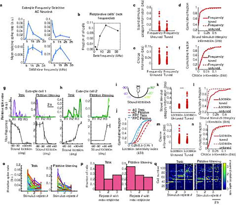
a, Mean responses (maximum relative spike rate across the 1 s sound presentation) to sinusoid amplitude-modulated (SAM) pure tones in example AC neurons. SAM tones were presented to passively listening mice after the task. b, Histogram of sound responsive cells’ best frequencies, the frequency of the maximum response for each neuron (unresponsive neurons were not included). c–f, Information about the sound stimulus category and the mouse’s choice in the task were compared between neurons that were untuned or tuned for sound stimulus frequency as measured in a. Significant tuning was defined by comparing the frequency selectivity index (y_max-y_mean)/(y_max+y_mean), where y_max is the mean response to the best frequency, and y_mean is the mean response to the other frequencies, to the frequency selectivity index calculated with shuffled trial identities. Frequency-tuned and untuned neurons did not contain significantly different amounts of information about the stimulus category or choice in the task (p > 0.5, rank sum test). g–h, In a subset of imaging experiments (n = 3), we played the same sound location stimuli as in the task, in a similar repeating pattern as mice experienced during task trials (three consecutive stimulus repeats). Trial-averaged responses to sound location stimuli measured during the task (left) and during passive listening (right) contexts. Line colors indicate the sound location (see panel i). (Bottom row) Tuning curves measured as the average maximal relative spike rate during the sound presentation at each sound location in task (left) and passive (right) contexts. i, Sound location color legend, applies to g,h. j, Cumulative distributions of sound location selectivity indices (LSI: (y_max-y_mean)/(y_max+y_mean), where y_max is the mean response to the best location, and y_mean is the mean response to the other locations) measured in AC and PPC neurons during the task (solid lines) and passive listening (dashed lines). AC cells had significantly higher LSIs than PPC cells (p < 0.001, rank sum test), and AC cells had significantly higher LSIs in the passive context than the active context (p < 0.001, signed rank test). k, Sound stimulus category information during the task in neurons untuned or tuned for sound location, determined by comparing LSIs in real and shuffled data during passive listening. Neurons with significant sound location tuning had more information about the sound location stimulus category (left vs right), p < 0.001, rank sum test. l, Cumulative distributions of sound category information for neurons tuned and untuned for sound location (using LSI significance). m, Choice information in neurons untuned or tuned for the sound location. n, Cumulative distributions of choice information for neurons tuned and untuned for the sound location (using LSI significance). Location-selective neurons had similar distributions of choice information (p > 0.5, rank sum test). o, Mean response of all neurons across each stimulus repeat during the task (left) and passive (right) contexts. Error bars indicate mean ± sem. Responses to sound repeat 1 tended to be higher than responses to repeats 2 and 3 (p < 0.001, signed rank test). p, Histograms of the stimulus repeat during which cells had their maximal responses during task (left) and passive listening (right) contexts. q, z-scored, trial-averaged activity of all AC neurons with 3 stimulus repeats in the passive context, sorted by time of peak mean activity and aligned to the time of the first sound onset. Responses during the task (left) and passive listening (right) were sorted by the time of peak response during the task. White vertical lines show the onset times of the first, second, and third sound stimulus repeats. Task trials with more or fewer than three repeats were excluded. The overall temporal pattern of activation across the AC population appeared similar in the two contexts, with a subset of neurons responding during the first sound stimulus presentation, and other neurons responding later, with some responses appearing to depend on subsequent sound stimulus repeats. Many neurons did not appear obviously responsive to the sound stimuli used in the task.

Extended Data Figure 2. GLM components, fit quality and model fit examples.

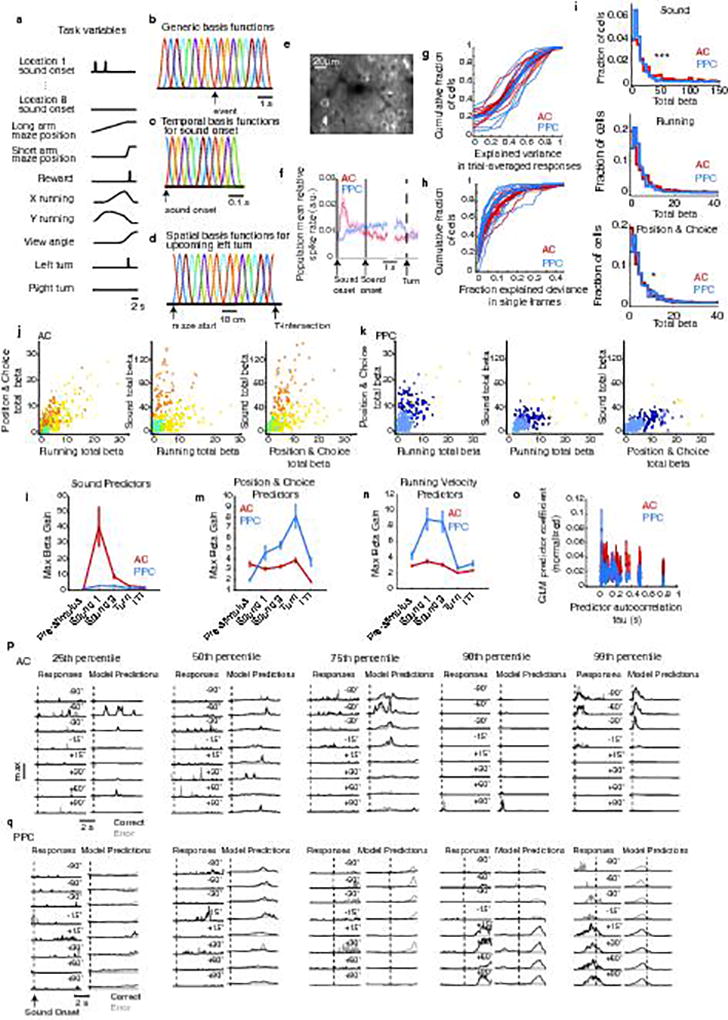
a, Time course of the behavior variables included in the GLM during an example trial, in which the sound stimulus was played from location 1 (−90 deg) and the mouse turned left at the T-intersection to receive a reward. Each predictor was convolved with a set of basis functions (Methods, examples in b–d). b, Generic set of basis functions that were convolved with behavior variables and events, extending backward and forward in time to model a neuron’s response to and prediction of events. The density, temporal extent, and width of basis functions were tailored to each behavioral variable (Methods). c, Example set of basis functions used for sound onset for each of 8 locations. These basis functions are shown before convolving with a vector that specifies sound onset time as a time series of zeros and ones (as shown in a). d, Example set of basis functions defined spatially along the extent of the stem of the T-maze, which were positive only when the mouse made a left turn in that trial. e, Example field of view showing GCaMP6 expression in PPC. f, Mean activity across all AC (red) and PPC (blue) cells, across all trials. Shading indicates s.e.m. n = 7 datasets for AC and PPC. g, Uncoupled encoding model performance measured using trial-averaged responses and predictions, quantified as explained variance. Each thin line is the distribution from a single dataset (n = 7 AC datasets, n = 7 PPC datasets). Thick lines indicate mean distributions across datasets. AC vs PPC: p > 0.1, rank sum test. h, Uncoupled encoding model performance measured as the fraction of additional explained deviance compared to the null model on frame-by-frame activity (Methods). Each thin line is the distribution from a single dataset. Thick lines indicate mean distributions across datasets. AC vs. PPC: p < 0.05, rank sum test. Note that explained deviance is calculated over single imaging frames and single trials in the test data set (not on averaged data), and because of trial-to-trial variability of neuron responses, does not approach perfect prediction (1.0). i, Histograms of distributions of total beta score (the sum of the absolute value of beta coefficients) in fitted models across all AC and PPC neurons, for predictors in three categories: 1) sound, 2) running, and 3) position/choice (turn direction in the maze). For ease of display, identically zero values were ignored when making the histograms. AC neurons tended to have stronger weights for predictors related to the sound stimulus (p < 0.001, rank sum test), while PPC neurons tended to have stronger weights for predictors related to position/choice (p < 0.05, rank sum test). j–k, Relationship of predictor weights within single neurons in AC and PPC. For each neuron, a score within each predictor category was calculated as the sum of the absolute value of coefficients (“total beta”). Clustering was used to reveal functional groups of neurons tuned to different sets of parameters (see Supplementary Information). Different clusters are indicated with different colors. Note that clustering was performed separately on AC and PPC data, hence the clusters obtained for AC are not related to those for PPC. l–n, Fitted model components’ gain⁴³ for variables related to running speed, position in the maze and turn direction, and sound location (exp(β*X), right, where β is the fitted coefficient, and X is the task predictor convolved with the basis functions), during the various epochs of the trial. mean ± s.e.m. o, Timescales of task predictors. A single exponential was fit to the autocorrelation of each of the 419 task predictors used in the uncoupled model, in order to estimate each variable’s timescale of variability. Across all AC (red) and PPC (blue) neurons, the mean coefficient magnitude fitted by the model for each task predictor was compared to the decay time constant, to determine whether the longer coding timescale in PPC could be explained by neurons in PPC responding preferentially to variables with longer timescales of variability. Even for task variables with longer timescales, AC tended to have greater coefficients (p < 0.001, rank sum test). It was thus unlikely that the longer coding timescales that we measured in PPC were due to its modulation by task variables with long timescales. p, Example AC responses and model predictions. Trial-averaged responses of example AC neurons during the sound stimulus presentation in correct (black) and error (gray) test trials (left) and the model’s predicted responses in left-out data (right). All responses were normalized to the maximum response across all trial conditions (y-axis scale) and aligned to the time of the first sound stimulus onset. Each row is the trial-averaged response or prediction for trials of one of the eight sound location conditions. Neurons with model fit performance across the spectrum are included, from poorly fit (25^th percentile), to very well-fit (99^th percentile). q, Same as p, for PPC

Extended Data Figure 3. Choice probability and behavioral relevance of sensory information.

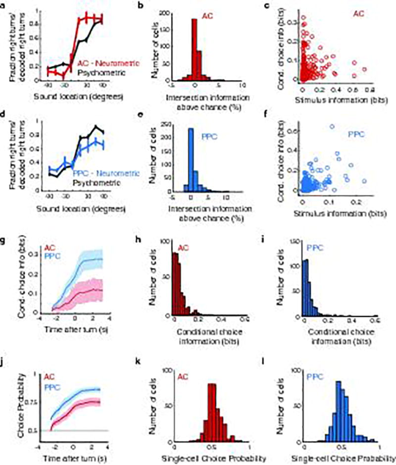
a, Red: AC neurometric curve computed from the performance of a sound location decoder (Supplementary Information). Dark gray: psychometric curve for mice from AC imaging sessions. Session-averaged psychometric and neurometric curves were positively correlated (r = 0.93, p < 0.001). b, Intersection information (II) above chance levels in AC neurons. The amount of II per cell above chance level was 0.2% ± 0.1% in AC (larger than zero with p < 0.0001, paired signed-rank test) and 0.7% ± 0.2% in PPC (p < 0.0001, paired signed-rank test). c, Conditional choice information plotted against stimulus information for all single AC cells. Stimulus information was computed without discounting the correlation between stimulus and choice (Spearman r = 0.33, p < 0.001; Supplementary Information). d–f, Same as a–c, except for PPC. d, Session-averaged psychometric and neurometric curves were positively correlated (r = 0.99, p < 0.001). e, Intersection information (II) above chance levels in PPC neurons was 0.7 ± 0.2 (p < 0.0001, paired signed rank test). f, Spearman r = 0.43, p < 0.001. g, Cumulative conditional choice information, computed by the performance of a choice decoder that assumes knowledge of all GLM predictors not directly related to choice (Supplementary Information). Cumulative conditional choice information was significant in both AC and PPC (AC: p < 0.05, PPC: p < 0.001, one-tailed t-test on the value of the choice information at the moment of the turn). Red: AC, blue: PPC. h–i, Total single-cell conditional choice information, computed as the maximum of the cumulative conditional choice information for each cell in AC and PPC. j–l, Same as g–i, quantifying the performance of the conditional choice decoder as a model-based choice probability¹⁹. j, Population choice probability was significantly larger than 0.5 in both AC and PPC at the last aligned time frame (p<0.001, one-tailed t-test). k, Mean single-cell choice probability 0.537±0.005 (larger than 0.5, p < 0.001, t-test). l: Mean single-cell choice probability 0.536±0.006 (larger than 0.5, p < 0.001, t-test).

Extended Data Figure 4. Decoder Controls.

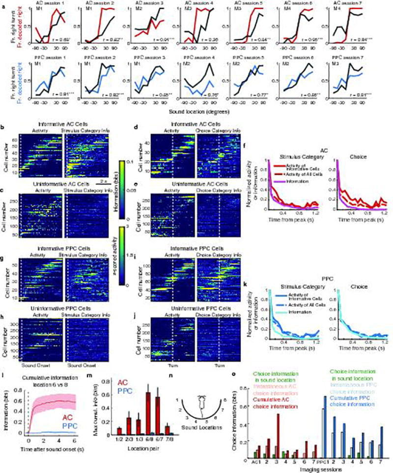
a, Gray: behavior performance during single imaging sessions used in all analyses. Overall behavior performance did not correlate with the number of choice selective neurons in the AC (r = −0.34, p > 0.1) or PPC (r = 0.38, p > 0.1) populations. Red, blue: single-session neurometric curves a sound location decoder (same as in Extended Data Fig. 3a, d; Supplementary Information). Inset in each panel reports the correlation coefficient between the neurometric and psychometric curves. * indicated p < 0.05; ** p < 0.01; *** p < 0.001; one-tailed test with null hypothesis that correlation is not higher than chance. b, (left) z-scored trial-averaged activity of all AC neurons with > 0.06 bits of stimulus information, sorted by time of peak mean activity, aligned to trial events as in (Fig. 1d,e). (right) Instantaneous stimulus category information in the same neurons. Time scalebar below panel on the right applies to all panels b–e and g–j. c, (left) z-scored, trial-averaged activity of all AC neurons with ≤ 0.06 bits of stimulus information. (right) Instantaneous stimulus category information in the same neurons. d, (left) z-scored, trial-averaged activity of all AC neurons with > 0.06 bits of choice information, sorted by time of peak mean activity. (right) Instantaneous choice information for the same cells. e, (left) z-scored, trial-averaged activity of all AC neurons with ≤ 0.06 bits of choice information, sorted by time of peak mean activity. (right) Instantaneous choice information for the same cells. f, Information about stimulus category (left, magenta) and choice (right, magenta) averaged across all AC neurons with at least 0.06 bits of information, as a function of the time from the peak. Normalized, aligned activity in all cells (dashed line) and informative cells (solid red line) are superimposed. g–k Same as b–f, for PPC cells. l–n, Information about the exact location of the sound stimulus. l, The cumulative population decoder was used on subsets of trials from only two sound locations such that there were equal numbers of trials from each location and no other locations were present. The data are shown for a comparison of locations 6 and 8. Note that locations 6 and 8 are part of the same category and indicate the same correct choice in the task. m, Maximum cumulative information calculated as in (l) for other location pairs that belong to the same stimulus category (left or right). All imaging experiments were performed in the left hemisphere, and so AC had higher information about contralateral sound stimulus locations. Error bars indicate mean ± sem. n, Diagram showing the sound location arrangements for location pairs compared in decoders in (l–m). o, Choice information in all datasets. Green bars: choice information that can be extracted from sound location due to an uneven distribution of errors across sound locations. This was a concern because more errors occurred at sound locations close to the midline (Fig. 1c), and perhaps location tuning could lead to an aberrant choice information measurement. Light red (AC) and light blue (PPC): maximum instantaneous choice information in neuronal population activity. Dark red (AC) and dark blue (PPC): total cumulative choice information in neuronal population activity. The uneven distribution of error trials across sound locations was not sufficient to explain choice information in AC or PPC.

Extended Data Figure 5. Coupling and Pearson correlations across contexts.

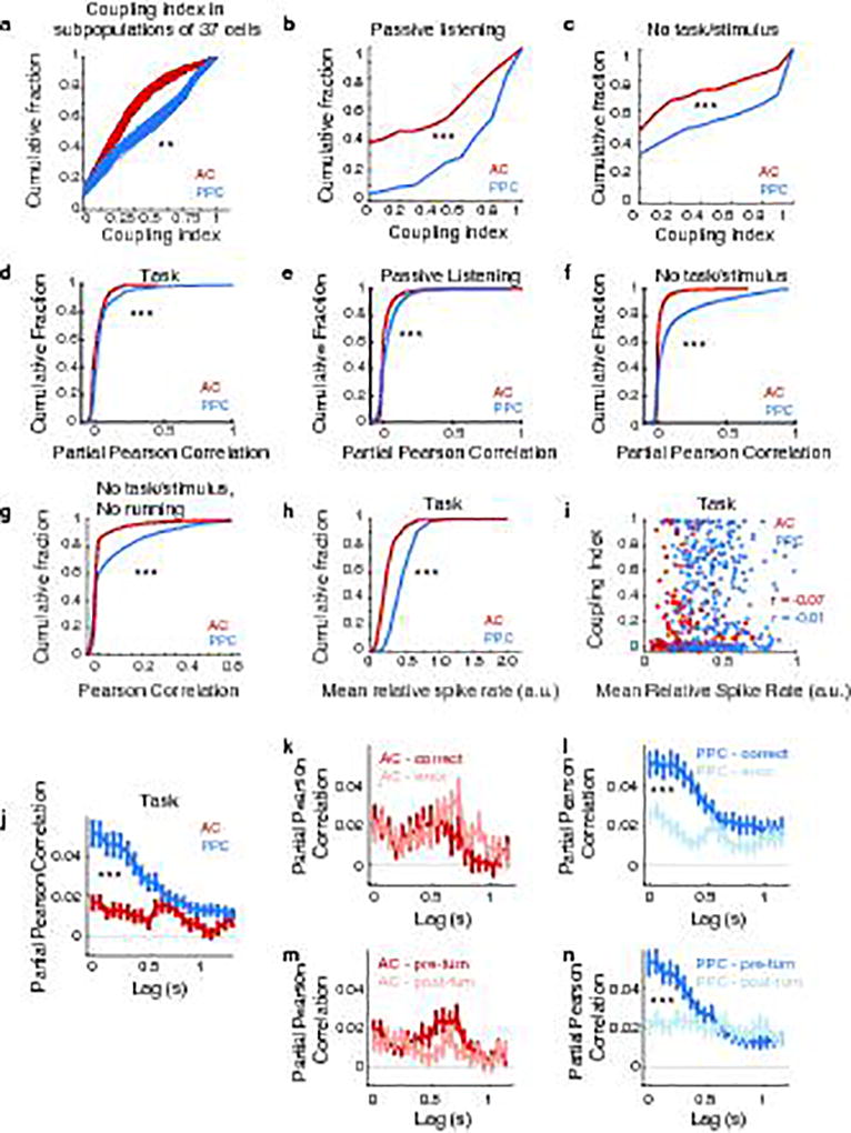
a, The coupled model was fit using random subpopulations of 37 neurons (the number of neurons in the smallest dataset) 100 times in all AC and PPC datasets. Cumulative distributions of performance of the coupled model using all subsamples of AC (red) and PPC (blue) datasets show that all PPC datasets still had greater coupling than all AC datasets (p < 0.01, rank sum test), even when using smaller numbers of neurons. b–c, Cumulative distributions of the coupling index in AC (red) and PPC (blue), measured during passive listening and the “no task/stimulus” context. d, Cumulative distributions of partial Pearson correlations (Methods) during the pre-turn period of the task in AC (red) and PPC (blue). Consistent with the higher coupling indices measured in PPC (Fig. 3d), correlations were higher in PPC than AC (p < 0.001, KS test). e, Cumulative distributions of partial Pearson correlations during passive listening to the stimulus sets used in the task in AC (red) and PPC (blue) datasets. PPC was more correlated than AC even when the mouse was not engaged in a task (p < 0.001; KS test). f, Cumulative distributions of partial Pearson correlations measured in the “no task/stimulus” context in AC (red) and PPC (blue). Again, PPC was more correlated than AC, in the absence of task or sound stimulus presentations (p < 0.001, KS test). g, Cumulative distributions of Pearson correlations measured in the “no task/stimulus” context when the mice were stationary (not running) on the ball (AC vs. PPC: p < 0.001, KS test). h, Cumulative distributions of mean relative spike rates in AC (0.24 ± 0.14 a.u., mean ± sem) and PPC (0.45 ± 0.18 a.u.). AC vs. PPC: p < 0.001, KS test. i, Coupling index vs. mean relative firing rate measured during the pre-turn period of the task. Each dot is one neuron. Because coupling and firing rate were not positively correlated (AC: r = −0.020; PPC: r = 0.007; p > 0.25), it is unlikely that higher firing rates in PPC caused an artefactual increase in correlation and coupling relative to AC. j, Partial Pearson correlations, computed across trials for time lags spanning 0 to over 1 s in AC (red) and PPC (blue), over all data, during the task. *** indicates p < 0.001, rank-rum test on the average Partial Pearson correlation across lags smaller than 0.5s. k, Partial Pearson correlations in AC populations, computed separately for correct (red) and error (pink) trials, for pre-turn data. l, Same as k, for PPC (dark blue: correct trials, light blue: error trials). *** indicates p < 0.001, rank-sum test on the average partial Pearson correlation across lags smaller than 0.5 s. m, Partial Pearson correlations in the pre-turn (red) and post-turn (pink) trial epochs in AC populations. n, Same as m, for PPC. *** indicates p < 0.001, rank-sum test on the average partial Pearson correlation across lags smaller than 0.5 s.

Extended Data Figure 6. Using the cell-cell model to test possible contributions of task features to coupling.

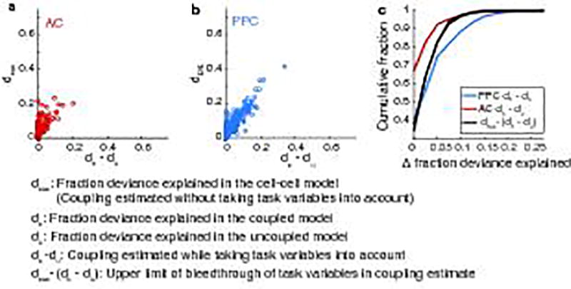
To help rule out the possibility that coupling parameters simply allow the model to explain behavioral correlates not included in the uncoupled model, rather than neuron-neuron correlations, we removed all the task predictors from our model to create a cell-cell model that only had coupling predictors. We reason that if the model could misattribute common drive to neurons by behavior variables, then the cell-cell model should be able to take on the uncoupled model’s prediction of responses to task parameters. We estimated an upper bound on the bleedthrough of task variables to coupling parameters by comparing the cell-cell model d_cxc to d_c − d_u, the increase in model performance when including coupling predictors in addition to the task predictors. If the coupling predictors could explain all of the responses related to the task predictors, d_cxc would far exceed the coupling value. a–b, Performance of a version of the encoding model with only the activity of other neurons as predictors and no task predictors (cell-cell model) compared to coupling (performance of coupled model – performance of uncoupled model) in AC (a) PPC (b). c, Comparing cumulative distributions of coupling in AC (red line) and PPC (blue line) to our estimates of an upper bound on the extent to which coupling could be explained entirely by task-related variables (black lines). Note that the coupling distribution in AC cells (red line) was mostly restricted to values less than the upper bound on coupling explainable by task-related variables, while coupling in many PPC neurons (blue line) exceeded it (p < 0.01, rank sum test). These results suggest that the higher level of coupling measured in PPC is unlikely to be due to shared common inputs to PPC neurons relating to task variables.

Extended Data Figure 7. Choice information redundancy.

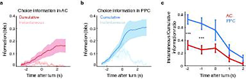
a–b, Cumulative (dark lines) and instantaneous (light lines) choice information in AC (n = 7 datasets) and PPC (n = 7 datasets), aligned to the turn and averaged across datasets. Shading indicates mean ± sem across datasets. c, Ratio of instantaneous to cumulative choice information in 1 s windows, relative to the time of the mouse’s turn in the maze. In PPC, instantaneous and cumulative information were similar prior to the turn. These results support our findings in Fig. 4, that information in PPC was consistent (here, redundant) across time before the mouse reported its choice by turning in the maze. *** indicates p < 0.001, z-test.

Extended Data Figure 8. Population scaling of information and consistency.

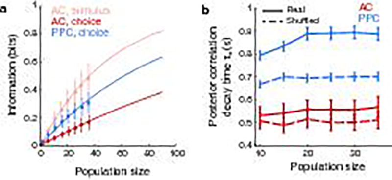
a, Scaling of total information content (maximum of cumulative information) with population size. Error bars indicate mean ± sem across datasets. Lines: analytical prediction from the Random Overlap model (Supplementary Information). b. Scaling of information consistency with population size, by measuring τ₂ (the long timescale component of decoder consistency, as in Fig. 4f) while varying population sizes (Supplementary Information). Error bars indicate mean ± sem across datasets. While information in AC and PPC grew with increasing population size, the coding timescale remained constant in AC, but grew modestly in PPC.

Extended Data Figure 9. Simple generative model of sequential neuronal activity and the effect of shuffling on information content.

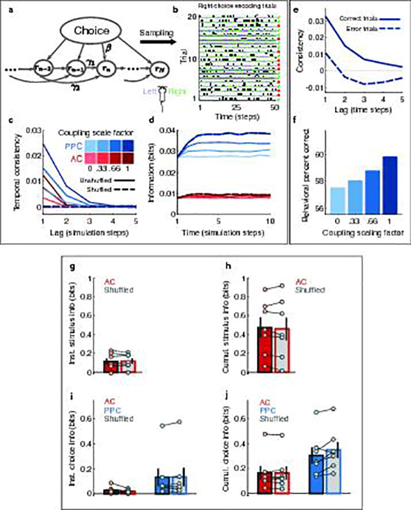
a, Schematic of simple model of choice tuning and statistical coupling between cells, expressed as a probabilistic graphical model. “Choice” indicates the choice encoded by the neuronal population in any given trial. r_i represents the activation of cell i, β is the strength of choice tuning, and γ₁ and γ₂ represent the strength of the statistical coupling of cell i to cell i − 1 and cell i − 2 respectively (Supplementary Information). b, Example of cell activity and decoded choice signal generated by the model for a batch of 20 trials encoding right choice. For each trial, the top row indicates the activity of left-preferring cells (black = active). The middle row indicates the activity of right-preferring cells. The bottom row indicates the choice decoded at each instant from the population activity (green = right, purple = left; Supplementary Information). Symbols on the right indicate whether the readout model implemented the correct choice. c, Temporal consistency computed across 10⁵ trials, each composed by 50 time steps. Different shades of red (or blue) indicate different multiplicative scaling factors applied to both coupling parameters γ_i, ranging from 0 for no coupling to 1 for the values derived from experimental data in AC (or PPC). Dashed lines: consistency computed for shuffled data (superimposed with the solid lines corresponding to no coupling). d, Same as c, for the instantaneous choice information contained in the choice signal generated by the model, over the first 10 time steps of the simulation. Note how cross-cell coupling enables accumulation of choice information. Note also how information in shuffled data is identical to the information in the unshuffled data. e, Temporal consistency for simulated PPC data, computed separately for behaviorally correct trials (solid line) and error trials (dashed line), as determined by the readout model described in Supplementary Information. f, Behavioral performance generated by the readout model (Supplementary Information) as a function of strength of the coupling in the model. 0 corresponds to no coupling; 1 to the value of the coupling parameters derived from the experimental data. g, Instantaneous stimulus information measured 1 s after the first stimulus onset, in real experimental data (red) and after disrupting coupling by shuffling the identities of trials of the same condition independently for each neuron (gray). Information was computed for random subpopulations of 37 cells and averaged across 48 such random selections. Circles represent individual datasets, bars represent the average across datasets, error bars represent mean ± sem. h, Same as g, for cumulative information at the last aligned time point in a trial. i, Same as g, for choice information in both AC (red) and PPC (blue) at the moment of the turn. j, Same as i, for cumulative information at the last aligned time point in the trial.

References

- 1.Hasson U, Chen J, Honey CJ. Hierarchical process memory: memory as an integral component of information processing. Trends Cogn Sci. 2015;19:304–313. doi: 10.1016/j.tics.2015.04.006. [DOI] [PMC free article] [PubMed] [Google Scholar]
- 2.Honey CJ, Thesen T, Donner TH, Silbert LJ, Carlson CE, Devinsky O, Doyle WK, Rubin N, Heeger DJ, Hasson U. Slow cortical dynamics and the accumulation of information over long timescales. Neuron. 2012;76:423–434. doi: 10.1016/j.neuron.2012.08.011. [DOI] [PMC free article] [PubMed] [Google Scholar]
- 3.Mauk MD, Buonomano DV. The neural basis of temporal processing. Annu Rev Neurosci. 2004;27:307–340. doi: 10.1146/annurev.neuro.27.070203.144247. [DOI] [PubMed] [Google Scholar]
- 4.Murray JD, Bernacchia A, Freedman DJ, Romo R, Wallis JD, Cai X, Padoa-Schioppa C, Pasternak T, Seo H, Lee D, Wang XJ. A hierarchy of intrinsic timescales across primate cortex. Nat Neurosci. 2014;17:1661–1663. doi: 10.1038/nn.3862. [DOI] [PMC free article] [PubMed] [Google Scholar]
- 5.Yang Y, Zador AM. Differences in sensitivity to neural timing among cortical areas. J Neurosci. 2012;32:15142–15147. doi: 10.1523/JNEUROSCI.1411-12.2012. [DOI] [PMC free article] [PubMed] [Google Scholar]
- 6.Buracas GT, Zador AM, DeWeese MR, Albright TD. Efficient discrimination of temporal patterns by motion-sensitive neurons in primate visual cortex. Neuron. 1998;20:959–969. doi: 10.1016/s0896-6273(00)80477-8. [DOI] [PubMed] [Google Scholar]
- 7.Yang Y, Deweese MR, Otazu GH, Zador AM. Millisecond-scale differences in neural activity in auditory cortex can drive decisions. Nat Neurosci. 2008;11:1262–1263. doi: 10.1038/nn.2211. [DOI] [PMC free article] [PubMed] [Google Scholar]
- 8.Shadlen MN, Newsome WT. Neural basis of a perceptual decision in the parietal cortex (area LIP) of the rhesus monkey. J Neurophysiol. 2001;86:1916–1936. doi: 10.1152/jn.2001.86.4.1916. [DOI] [PubMed] [Google Scholar]
- 9.Andersen RA, Cui H. Intention, action planning, and decision making in parietal-frontal circuits. Neuron. 2009;63:568–583. doi: 10.1016/j.neuron.2009.08.028. [DOI] [PubMed] [Google Scholar]
- 10.Harvey CD, Coen P, Tank DW. Choice-specific sequences in parietal cortex during a virtual-navigation decision task. Nature. 2012;484:62–68. doi: 10.1038/nature10918. [DOI] [PMC free article] [PubMed] [Google Scholar]
- 11.Jenkins WM, Merzenich MM. Role of cat primary auditory cortex for sound-localization behavior. J Neurophysiol. 1984;52:819–847. doi: 10.1152/jn.1984.52.5.819. [DOI] [PubMed] [Google Scholar]
- 12.Nakamura K. Auditory spatial discriminatory and mnemonic neurons in rat posterior parietal cortex. J Neurophysiol. 1999;82:2503–2517. doi: 10.1152/jn.1999.82.5.2503. [DOI] [PubMed] [Google Scholar]
- 13.McNaughton BL, Mizumori SJ, Barnes CA, Leonard BJ, Marquis M, Green EJ. Cortical representation of motion during unrestrained spatial navigation in the rat. Cereb Cortex. 1994;4:27–39. doi: 10.1093/cercor/4.1.27. [DOI] [PubMed] [Google Scholar]
- 14.Nitz DA. Tracking route progression in the posterior parietal cortex. Neuron. 2006;49:747–756. doi: 10.1016/j.neuron.2006.01.037. [DOI] [PubMed] [Google Scholar]
- 15.Raposo D, Kaufman MT, Churchland AK. A category-free neural population supports evolving demands during decision-making. Nat Neurosci. 2014;17:1784–1792. doi: 10.1038/nn.3865. [DOI] [PMC free article] [PubMed] [Google Scholar]
- 16.Whitlock JR, Pfuhl G, Dagslott N, Moser M-B, Moser EI. Functional split between parietal and entorhinal cortices in the rat. Neuron. 2012;73:789–802. doi: 10.1016/j.neuron.2011.12.028. [DOI] [PubMed] [Google Scholar]
- 17.Hanks TD, Kopec CD, Brunton BW, Duan CA, Erlich JC, Brody CD. Distinct relationships of parietal and prefrontal cortices to evidence accumulation. Nature. 2015;520:220–223. doi: 10.1038/nature14066. [DOI] [PMC free article] [PubMed] [Google Scholar]
- 18.Graf AB, Andersen RA. Predicting oculomotor behaviour from correlated populations of posterior parietal neurons. Nat Commun. 2015;6:6024. doi: 10.1038/ncomms7024. [DOI] [PMC free article] [PubMed] [Google Scholar]
- 19.Park IM, Meister ML, Huk AC, Pillow JW. Encoding and decoding in parietal cortex during sensorimotor decision-making. Nat Neurosci. 2014;17:1395–1403. doi: 10.1038/nn.3800. [DOI] [PMC free article] [PubMed] [Google Scholar]
- 20.Pillow JW, Shlens J, Paninski L, Sher A, Litke AM, Chichilnisky EJ, Simoncelli EP. Spatio-temporal correlations and visual signalling in a complete neuronal population. Nature. 2008;454:995–999. doi: 10.1038/nature07140. [DOI] [PMC free article] [PubMed] [Google Scholar]
- 21.Panzeri S, Harvey CD, Piasini E, Latham PE, Fellin T. Cracking the Neural Code for Sensory Perception by Combining Statistics, Intervention, and Behavior. Neuron. 2017;93:491–507. doi: 10.1016/j.neuron.2016.12.036. [DOI] [PMC free article] [PubMed] [Google Scholar]
- 22.Hromadka T, Zador AM. Representations in auditory cortex. Curr Opin Neurobiol. 2009;19:430–433. doi: 10.1016/j.conb.2009.07.009. [DOI] [PMC free article] [PubMed] [Google Scholar]
- 23.Averbeck BB, Latham PE, Pouget A. Neural correlations, population coding and computation. Nat Rev Neurosci. 2006;7:358–366. doi: 10.1038/nrn1888. [DOI] [PubMed] [Google Scholar]
- 24.Carnevale F, de Lafuente V, Romo R, Parga N. An optimal decision population code that accounts for correlated variability unambiguously predicts a subject's choice. Neuron. 2013;80:1532–1543. doi: 10.1016/j.neuron.2013.09.023. [DOI] [PubMed] [Google Scholar]
- 25.Harris KD, Barthó P, Chadderton P, Curto C, de la Rocha J, Hollender L, Itskov V, Luczak A, Marguet SL, Renart A, Sakata S. How do neurons work together? Lessons from auditory cortex. Hear Res. 2011;271:37–53. doi: 10.1016/j.heares.2010.06.006. [DOI] [PMC free article] [PubMed] [Google Scholar]
- 26.Cohen MR, Maunsell JHR. Attention improves performance primarily by reducing interneuronal correlations. Nature Neuroscience. 2009;12:1594–1600. doi: 10.1038/nn.2439. [DOI] [PMC free article] [PubMed] [Google Scholar]
- 27.Ecker AS, Berens P, Keliris GA, Bethge M, Logothetis NK, Tolias AS. Decorrelated Neuronal Firing in Cortical Microcircuits. Science. 2010;327:584–587. doi: 10.1126/science.1179867. [DOI] [PubMed] [Google Scholar]
- 28.Okun M, Steinmetz NA, Cossell L, Iacaruso MF, Ko H, Bartho P, Moore T, Hofer SB, Mrsic-Flogel TD, Carandini M, Harris KD. Diverse coupling of neurons to populations in sensory cortex. Nature. 2015;521:511–515. doi: 10.1038/nature14273. [DOI] [PMC free article] [PubMed] [Google Scholar]
- 29.Rabinowitz NC, Goris RL, Cohen M, Simoncelli EP. Attention stabilizes the shared gain of V4 populations. Elife. 2015;4:e08998. doi: 10.7554/eLife.08998. [DOI] [PMC free article] [PubMed] [Google Scholar]
- 30.Bathellier B, Ushakova L, Rumpel S. Discrete neocortical dynamics predict behavioral categorization of sounds. Neuron. 2012;76:435–449. doi: 10.1016/j.neuron.2012.07.008. [DOI] [PubMed] [Google Scholar]
- 31.Harvey CD, Collman F, Dombeck DA, Tank DW. Intracellular dynamics of hippocampal place cells during virtual navigation. Nature. 2009;461:941–946. doi: 10.1038/nature08499. [DOI] [PMC free article] [PubMed] [Google Scholar]
- 32.Aronov D, Tank DW. Engagement of neural circuits underlying 2D spatial navigation in a rodent virtual reality system. Neuron. 2014;84:442–456. doi: 10.1016/j.neuron.2014.08.042. [DOI] [PMC free article] [PubMed] [Google Scholar]
- 33.Elhilali M, Fritz JB, Klein DJ, Simon JZ, Shamma SA. Dynamics of precise spike timing in primary auditory cortex. J Neurosci. 2004;24:1159–1172. doi: 10.1523/JNEUROSCI.3825-03.2004. [DOI] [PMC free article] [PubMed] [Google Scholar]
- 34.Pulkki V. Virtual Sound Source Positioning Using Vector Base Amplitude Panning. JAES. 1997;45:10. [Google Scholar]
- 35.Creutzfeldt O, Hellweg FC, Schreiner C. Thalamocortical transformation of responses to complex auditory stimuli. Exp Brain Res. 1980;39:87–104. doi: 10.1007/BF00237072. [DOI] [PubMed] [Google Scholar]
- 36.Greenberg DS, Kerr JN. Automated correction of fast motion artifacts for two-photon imaging of awake animals. J Neurosci Methods. 2009;176:1–15. doi: 10.1016/j.jneumeth.2008.08.020. [DOI] [PubMed] [Google Scholar]
- 37.Vogelstein JT, Packer AM, Machado TA, Sippy T, Babadi B, Yuste R, Paninski L. Fast nonnegative deconvolution for spike train inference from population calcium imaging. J Neurophysiol. 2010;104:3691–3704. doi: 10.1152/jn.01073.2009. [DOI] [PMC free article] [PubMed] [Google Scholar]
- 38.McCullagh P, Nelder JA. Generalized linear models. 2. Chapman and Hall; 1989. [Google Scholar]
- 39.Lee DD, Seung HS. Learning the parts of objects by non-negative matrix factorization. Nature. 1999;401:788–791. doi: 10.1038/44565. [DOI] [PubMed] [Google Scholar]
- 40.Friedman J, Hastie T, Tibshirani R. Regularization paths for Generalized Linear Models via coordinate descent. J Stat Softw. 2010;33:1–22. [PMC free article] [PubMed] [Google Scholar]
- 41.Agresti A. Categorical data analysis. 3. Wiley; 2013. [Google Scholar]
- 42.Quian Quiroga R, Panzeri S. Extracting information from neuronal populations: information theory and decoding approaches. Nat Rev Neurosci. 2009;10:173–185. doi: 10.1038/nrn2578. [DOI] [PubMed] [Google Scholar]
- 43.Shannon CE. A mathematical theory of communication. AT&T Bell Lab Tech J. 1948;27:379–423. [Google Scholar]
- 44.Panzeri S, Treves A. Analytical estimates of limited sampling biases in different information measures. Network: Computation in Neural Systems. 1996;7:87–107. doi: 10.1080/0954898X.1996.11978656. [DOI] [PubMed] [Google Scholar]
Associated Data
This section collects any data citations, data availability statements, or supplementary materials included in this article.