

Abstract
Transfer learning in deep convolutional neural networks (DCNNs) is an important step in its application to medical imaging tasks. We propose a multi-task transfer learning DCNN with the aims of translating the ‘knowledge’ learned from non-medical images to medical diagnostic tasks through supervised training and increasing the generalization capabilities of DCNNs by simultaneously learning auxiliary tasks. We studied this approach in an important application: classification of malignant and benign breast masses. With IRB approval, digitized screen-film mammograms (SFMs) and digital mammograms (DMs) were collected from our patient files and additional SFMs were obtained from the Digital Database for Screening Mammography. The data set consisted of 2,242 views with 2,454 masses (1,057 malignant, 1,397 benign). In single-task transfer learning, the DCNN was trained and tested on SFMs. In multi-task transfer learning, SFMs and DMs were used to train the DCNN, which was then tested on SFMs. N-fold cross-validation with the training set was used for training and parameter optimization. On the independent test set, the multitask transfer learning DCNN was found to have significantly (p=0.007) higher performance compared to the single-task transfer learning DCNN. This study demonstrates that multitask transfer learning may be an effective approach for training DCNN in medical imaging applications when training samples from a single modality are limited.
Keywords: digitized screen-film mammography, digital mammography, computer-aided diagnosis, mass, transfer learning, multi-task learning, deep convolutional neural network
1. INTRODUCTION
Transfer learning and multi-task learning are machine learning methods aiming at generalization to new classes, tasks or distributions.(Bengio, 2012; Deng and Yu, 2014) Transfer learning is a deep learning technique used to transfer the knowledge learned from the source tasks to the target tasks. Multitask learning is based on the assumption that learning interrelated concepts might force the classification methods to develop broad generalizations resulting in improved performance compared to single-task learning.(Caruana, 1998) In this work, we propose an approach with the aim to interpret medical imaging tasks through transfer learning while improving the generalization capabilities by learning auxiliary tasks.
In a trained deep convolutional neural network (DCNN), the first layer features are generic, in the sense that they are not task specific, and the last layer features are specific to the task with a gradual transition from generic to specific in the middle layers forming a hierarchical multilayer architecture.(Yosinski et al., 2014) In a transfer learning approach for DCNNs, the first few generic layers of a DCNN trained on source data are copied to a DCNN to be trained on the target data where source and target data can be from different imaging domains. The specific layers in the target DCNN are randomly initialized and fine-tuned to the target task.(Tajbakhsh et al., 2016; Shin et al., 2016) This approach in medical imaging is largely motivated by the lack of large data sets for training deep and wide convolutional neural networks (CNNs). Transfer learning also has the potential to help improve the convergence rate by speeding up the target learning tasks and improve the generalization capability that will lead to better independent test performance in comparison to training DCNNs without transfer learning.(Torrey and Shavlik, 2009). A review article by Pan and Yang on transfer learning gives a survey of different types of transfer learning approaches and its applications.(Pan and Yang, 2010)
Our goal of using transfer learning is to append the “knowledge” of vast number of features learned through non-medical images to the “interpretation” of medical images via fine-tuning. This type of knowledge transfer is extensively studied in the machine learning field with many rapid new developments.(Pan and Yang, 2010; Fernando et al., 2017) In this study, we use inductive variation of transfer learning (Pan and Yang, 2010) where the source and the target tasks are different and completely labeled, i.e., ImageNet DCNN is trained to classify 1000 class daily life images while the target task is classification of masses on mammograms into two classes. Multi-task learning has been widely studied in machine learning with many studies showing increased performance compared to learning a single task.(Argyriou et al., 2007) This type of learning in CNNs is also sometimes referred to as parameter sharing (Bengio, 2012) or a feature-representation-transfer type of inductive transfer learning method.(Pan and Yang, 2010)
A recent article from Litjens et al (Litjens et al., 2017) provides an excellent review of the current trends in application of deep learning techniques to medical image analysis. In breast imaging, CNNs have been used in mammography for segmentation, detection, diagnosis of masses and breast density risk assessment. The first implementation of CNN for mammography was for classification of microcalcifications (Chan et al., 1993; Chan et al., 1995b) and masses using CNN and texture features (Chan et al., 1994; Sahiner et al., 1996) in computer-aided detection systems for these breast lesions.
In this study, we investigated the training of DCNN for computer-aided classification of malignant and benign masses on mammograms with transfer learning from non-medical images while simultaneously learning multiple related tasks. Classification of masses from digitized-screen film mammography (SFM) and digital mammography (DM) from two sources were treated as multiple but similar tasks for transfer leaning of the DCNN. Our goal is to understand the process of adapting the deep and wide CNNs to medical imaging tasks using available data, as well as the differences in multi-task and single-task transfer learning. N-fold cross-validation with the training set was used to study the effects of stochastic initializations and different levels of transfer learning, and the feature distributions at different layers of a trained DCNN were analyzed with a dimensionality reduction technique.
The manuscript is organized as follows: Section 2 describes the three heterogeneous mammography data sets from two sources for training and testing DCNN, the DCNN architecture, our approach to transfer learning, cross-validation in the training and validation data sets and sensitivity analysis of the selection of the best transfer network, Section 3 describes the results for various analyses and the independent test results, Section 4 discusses our observations from the results and conclusion.
2. MATERIALS AND METHODS
Fig. 1. gives an overview of our approach to train a DCNN using transfer learning for classification of masses on SFM. The experimental setup is broadly divided into three stages: (a) finding the representative N-fold split of the training set in transfer learning, (b) compare multi-task transfer learning to single-task transfer learning and finding the best N-fold classifier and (c) verify the training/validation observations using an independent test set.
Fig. 1.

Overview of our process to train DCNN using transfer learning from digitized screen-film mammograms (SFM) from two sources (UM and DDSM) and digital mammograms (DM).
2. 1. Data sets
For this study, three sets of mammography data were collected from two different sources. A total of 1,655 SFM views and 310 DM views were collected with the approval of the Institutional Review Board (IRB) at the University of Michigan Health System (UM). Another 277 SFM views were collected from the Digital Database for Screening Mammography (DDSM).(Heath et al., 2001) The DM images were acquired with a GE Senographe 2000D FFDM system at a pixel size of 100 μm x 100 μm and 14 bits/pixel. The DM data was acquired at UM from the year 2001 to 2006. The patient’s age ranged from 24 to 82 with a mean of 51.7 years. The mammograms for the SFM-UM set were digitized using a Lumiscan 85 laser scanner with an optical density range of 0–4.0. The SFM-DDSM set were acquired using a Lumisys 200 laser scanner with an optical density range of 0–3.6. Both sets of the SFM images were digitized at 12 bits/pixel. Table 1 and 2 summarize the data set information, the number of views and lesions in each image set and the distribution of malignant and benign cases. To simplify the notations in the following discussion, we will refer to the three types of data set, SFM-UM, SFM-DDSM, and DM-UM as SFM, DDSM, and DM, respectively. The 1,655 SFM views are divided by case into a training set of 748 views and an independent test set of 907 views. For each mass on each view, a bounding box was marked by a Mammography Quality Standards Act (MQSA) qualified radiologist with over 30 years of experience in breast imaging, using all the available clinical information. The DM images were acquired in raw format at 14 bits/pixel and processed using simple inverse logarithmic transformation and scaled to 12 bits/pixel. (Burgess, 2004) All images were downsampled to 200 μm x 200 μm resolution by averaging adjacent N x N pixels, where N depends on the original image pixel size. A previously developed background correction method was used to normalize the background gray levels that depended on the overlapping breast tissue and to reduce the variations due to x-ray exposure conditions. The background correction also had the advantage of normalizing the SFM and DM data sets. Detailed information of the method can be found elsewhere (Chan et al., 1995a; Sahiner et al., 1996), and our previous work (Samala et al., 2016) includes additional information on the results for background correction on SFM, DDSM, DM and digital breast tomosynthesis.
Table 1.
Mammography data sets used in this study
| Data type | Source | Device | Acquisition years | Gray level range | Optical density range | Pixel Size (μm) |
|---|---|---|---|---|---|---|
| SFM-UM | University of Michigan | Lumiscan 85 laser scanner | 1990 – 2005 | 12 bits | 0 – 4.0 | 50 × 50 |
| SFM-DDSM | Digital Database for Screening Mammography | Lumisys 200 laser scanner | 1988 – 1999 | 12 bits | 0 – 3.6 | 50 × 50 |
| DM-UM | University of Michigan | GE Senographe 2000D FFDM | 2001 – 2006 | 14 bits | NA | 100 × 100 |
Table 2.
Data sets used in this study. SFM-UM and DM-UM: digitized screen-film mammograms and digital mammograms from University of Michigan, SFM-DDSM: digitized-screen film mammograms from University of South Florida public data set. ROI: region-of-interest of size 128 x 128 pixels. Each ROI was flipped and rotated four times to obtain eight augmented samples.
| Data type | No. of views | No. of lesions | No. of malignant | No. of benign | No. of ROIs after data augmentation |
|---|---|---|---|---|---|
| Training Set | |||||
| SFM-UM | 748 | 886 | 317 | 569 | 7,088 |
| SFM-DDSM | 277 | 322 | 191 | 131 | 2,576 |
| DM-UM | 310 | 337 | 96 | 241 | 2,696 |
| Test Set | |||||
| SFM-UM | 907 | 909 | 453 | 456 | 7,272 |
| Total | 2,242 | 2,454 | 1,057 | 1,397 | 19,632 |
2. 2. Deep Convolutional Neural Networks
In this study, we used the DCNN network developed for the ImageNet LSVRC-2010 (Krizhevsky et al., 2012) contest in which 1.2 million images were classified into 1000 classes. The architecture won the ILSVRC-2012 competition with a top-5 error rate of 15.3%. This architecture was extensively studied and used for many transfer learning tasks among other networks such as VGG, ZFnet, GoogLeNet and Microsoft ResNet.(Zeiler and Fergus, 2014; Simonyan and Zisserman, 2014; Szegedy et al., 2015; He et al., 2016) Most of these networks other than ImageNet and ZFnet, are very deep with complex architecture; it is difficult to analyze the intermediate steps and will require long computation time to find the optimal approach for transfer learning. Hence we chose to use ImageNet for transfer learning to classify masses on mammograms. The CUDA-CONVNET2 software package (Krizhevsky et al., 2012) was trained on an NVIDIA Tesla K40 GPU.
The ImageNet DCNN contains five convolutional layers and three fully connected layers with rectified linear units, max-pooling layers and local response normalization layer, as shown in fig. 2. The structure characteristics are shown in Table 3. ImageNet was trained with an input region-of-interest (ROI) size of 256 x 256 pixels RGB channel while the extracted mammographic ROIs were 128 x 128-pixel gray-scale images. Using a 128 x 128 input in place of a 256 x 256 input would not affect the convolution layer setup except for the fully connected layers due to the change in the number of connections between the last convolution layer and the first fully connected layer. We could therefore freeze the weights of the ImageNet at the first n convolution layers to carry the pre-trained features from these layers for transfer learning while re-training the remaining convolution layers and the fully connected layers even when the input ROI size was different from 256 x 256 pixels. The 128 x 128 ROIs were repeated into the 3 channels and passed as input to the DCNN for transfer learning. Data augmentation and dropout methods were used to reduce overfitting. Each ROI was flipped and rotated four times to obtain eight augmented samples per ROI. For our malignant-versus-benign mass classification task in mammography, two additional fully connected layers (fc100 and fc2) were added to the ImageNet structure to drop down the 1000-node fully connected layer to a 2-node softmax classifier. All the fully connected layer weights and biases were randomly initialized for retraining. Stochastic gradient descent was used with a batch size of 128 samples, momentum of 0.9, weight decay of 0.0005 and base learning rate of 0.001 exponentially reducing to 0.00004. Only the learning rate was adjusted heuristically for the mammography training while the rest of the parameters were set based on the work by Krizhevsky et al.(Krizhevsky et al., 2012) Since none of the transfer networks were trained from scratch, we observed that 200 iterations were sufficient for the training and validation to stabilize. The training epochs was therefore fixed at 200 iterations for all conditions.
Fig. 2.
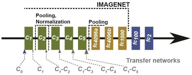
ImageNet DCNN structure used for transfer learning with the addition of two fully connected layers (fc100 and fc2) to be used with the mammography data. The six transfer networks are indicated at the five convolution layers. A transfer network re-trained with Ci to Cj convolution layers frozen is denoted by Ci-Cj. C0 denotes that none of the layers was frozen.
Table 3.
DCNN structure showing the number of weights, biases and parameters.
| Layer | Number of nodes | Filter size |
|---|---|---|
| C1 | 64 | 11 × 11 |
| C2 | 192 | 5 × 5 |
| C3 | 384 | 3 × 3 |
| C4 | 256 | 3 × 3 |
| C5 | 256 | 3 × 3 |
| F1 | 4096 | |
| F2 | 4096 | |
| F3 | 1000 | |
| F4 | 100 | |
| F5 | 2 | |
| Total | 10,446 |
2. 3. Transfer Learning and Sensitivity Analysis
For transfer learning with the ImageNet (fig. 2), we first studied how many of the convolution layers should be frozen during training with mammography data. DCNN is a hierarchical multilayer architecture where the early layers are more generic and the deeper layers are more specific. The generic layers are typically used to extract local edge features which are similar to Gabor filters. When a pre-trained DCNN structure is fine-tuned with transfer learning, the layers have to be frozen consecutively in order so that any weight updates in the early layers that are not frozen can be propagated to the weight updates in deeper layers. Hence, for our current DCNN structure, we compared six transfer networks (C0, C1, C1–C2, C1–C3, C1–C4 and C1–C5), where Ci–Cj denotes a CNN retrained with the weights in the Ci to Cj convolution layers frozen, and C1 and C0 denotes a CNN retrained with only the weights in C1 or none (C0) of the convolution layers frozen, respectively. Transfer learning can result in an increase in performance (positive transfer) or decrease in performance (negative transfer) in the target task. Analyzing the performance difference while changing the depth at which the convolution layers are frozen will identify the best among the studied transfer networks for the target task and may indicate what levels of generic to specific features are useful. To assess the robustness of the DCNN network for classifying benign and malignant masses and the dependence on the stochastic initialization of the DCNN weights and biases, the experiments were repeated for multiple random seeds. For N-fold case-based cross validation described in Section 2.4, the experiments were repeated for two random seeds, and all the cross-validation experiments were repeated for ten random seeds. The mean and standard deviation of the performance measures were presented where applicable.
2. 4. N-fold case-based cross-validation
For N-fold cross-validation, the stratified partitioning can be performed manually or automatically using a random seed. We split the malignant and benign data sets separately by case into four partitions randomly ten times using ten random seeds. A partition of malignant cases and a partition of benign cases were combined to form a random partition so that the proportions of malignant and benign cases were kept similar in the four random partitions each time. The motivation behind analyzing different random splits is to select a split that is more uniform and representative of the entire data set used in this study. The observed trends from the four folds are then expected to be more consistent across the subsequent experiments.
2.5. Multi-task transfer learning
Multi-task learning has for a long time been associated with the assumption that multiple-class associations can be used to constrain the learning towards a better solution and also is characterized as an innovative way to introduce knowledge into a high-capacity network.(Intrator and Edelman, 1996) In multi-task transfer learning, the objective is to simultaneously learn multiple related tasks and exploit their similarity to improve the performance in comparison to a single-task transfer learning. For this study, our multiple tasks were classification of malignant and benign breast masses on three similar but different image sets (SFM, DDSM, and DM). The heterogeneous data from DDSM and DM are added into each N-fold SFM data during transfer learning. Multi-task learning assumes that the learning tasks share features. In our study with the three image types, the domain is the same among the tasks and the target being classified is breast mass but acquired using different imaging technologies.
2. 6. Validation methods
To visualize the distribution of features extracted at different fully connected layers, we used the t-Distributed Stochastic Neighbor Embedding (t-SNE) method. It is an unsupervised dimensionality reduction technique that maps the distance relationships between multidimensional feature vectors to a two-dimensional rotation-invariant Euclidean space. Similar clusters are represented by closer points while dissimilar clusters are represented by distant points. It is particularly suited for visualizing high-dimensional correlated data that lie on several different low-dimensional manifolds (Maaten and Hinton, 2008). We used the t-SNE technique to visualize the high-dimensional features extracted from a fully connected layer of DCNN for mass images representing malignant and benign classes acquired with slightly different technologies or image devices.
The classification performance of DCNN in each cross-validation fold and in the independent test set were assessed using receiver operating characteristic (ROC) curves. A ‘proper’ binormal model of the ROC analysis (Metz and Pan, 1999) implemented in ROCKIT version 1.B2 (August 2006) was used to fit the ROC curves and to evaluate the statistical significance difference between the ROC curves. Both view-based and lesion-based ROC curves were calculated. For view-based analysis, each lesion on each view was counted as a single target, and for lesion-based analysis, each lesion on all views of each case was counted as a single target and the scores from all views of a given lesion were averaged to obtain a lesion-based score. In all analyses, the average score of the eight augmented samples from each ROI was used as the score of the ROI.
3. RESULTS
3. 1. N-fold split for training/validation
For the selection of a representative split for the N-fold case-based cross-validation, we used the SFM data with two transfer networks, C1 and C1–C3. For each random fold split, the DCNN training and validation was repeated for two stochastic initialized DCNNs. Fig. 3 shows the two validation AUC values of each fold for the ten random splits. We chose the random split N2 from the graph as the representative split based on the relatively small variation across the four folds and the relatively high average AUC within each split. N2 was then used for all transfer networks in the subsequent analyses.
Fig. 3.

Variation of the validation AUCs among 10 random splits for the four-fold case-based cross-validation and repeated DCNN training using two random initializations. (a) The ImageNet structure is frozen for C1 layer only. (b) The ImageNet structure is frozen for C1–C3 layers.
3. 2 Transfer learning
We investigated six transfer networks using cross-validation and sensitivity analysis. Cross-validation for each of the transfer networks was performed for ten stochastic initializations using the chosen N-fold split of the SFM training set (N2). The mean and the standard deviation of the validation AUC estimated from the 10 repeated experiments for the six transfer networks are shown in fig. 4. The transfer network C1 consistently performed better than other networks for three but worse for one of the four folds. The variation in the average AUC over the four folds obtained with C1 was the lowest among the six transfer networks.
Fig. 4.

Performance measure of each validation fold in the N-fold case-based cross-validation across the six transfer networks studied.
3. 3. Multi-task transfer learning and Independent testing
For the results discussed above, single-task transfer learning with only the SFM training set was used for retraining the ImageNet DCNN. For the multi-task transfer learning, we used the SFM training set together with the DDSM and DM data sets for retraining. In the latter experiments, during the cross-validation, the SFM training set was split into N-folds but the DDSM and DM data were appended in its entirety to each fold. The premise to this variation is that our final goal is to test the performance on an independent SFM set only.
To visualize the geometric representation of the features extracted at different fully-connected layers using the t-SNE technique, we varied the perplexity parameter, which is the approximate number of nearest neighbor masses associated with a given cluster, in the range of 10 to 100. Perplexity of value 30 was then chosen because consistent mapping of the features was observed between 30 and 100. We experimentally chose the t-SNE parameters including the learning rate (η), number of iterations, and momentum (α) to be 500, 5000 and 0.5, respectively, and the t-SNE was repeated ten times with different random seeds. The mapping with the lowest value of the cost function was chosen for analysis. The average feature score from eight flipped-and-rotated augmented version of each ROI was used as the feature value of each sample for this analysis. Fig. 5 shows the t-SNE plots of the structure and embedding relationships between the malignant-vs-benign and SFM-vs-DM-vs-DDSM training samples at the four fully connected feature layers for the single-task and multi-task approaches. Note that all t-SNE plots are shown without axes because the values on the axes do not have any intrinsic meaning; the main application of the method is for visualization of high-dimensional feature spaces.
Fig. 5.

2D t-SNE maps of the training samples obtained from the single-task and multi-task approaches for transfer networks at four fully connected layers. The legend indicates malignant and benign classes and SFM, DM, and DDSM data sets.
After the selection of CNN re-training scheme and feature analysis described above, the selected C1 transfer network was re-trained on the entire available training/validation data to maximize the training samples before final testing on the independent test set. The output of the DCNN softmax function was used as the decision variable to generate ROC curves. The view-based and lesion-based ROC curves for the independent test set are shown in fig. 6. To visualize the features in the DCNN, we used the deconvolutional network (Zeiler and Fergus, 2014) to project the features back to the input image space for the five convolutional layers as shown in fig. 7. The number of feature maps is equal to the number of convolution kernels in each layer but only six feature maps per layer are shown as examples for each mass.
Fig. 6.
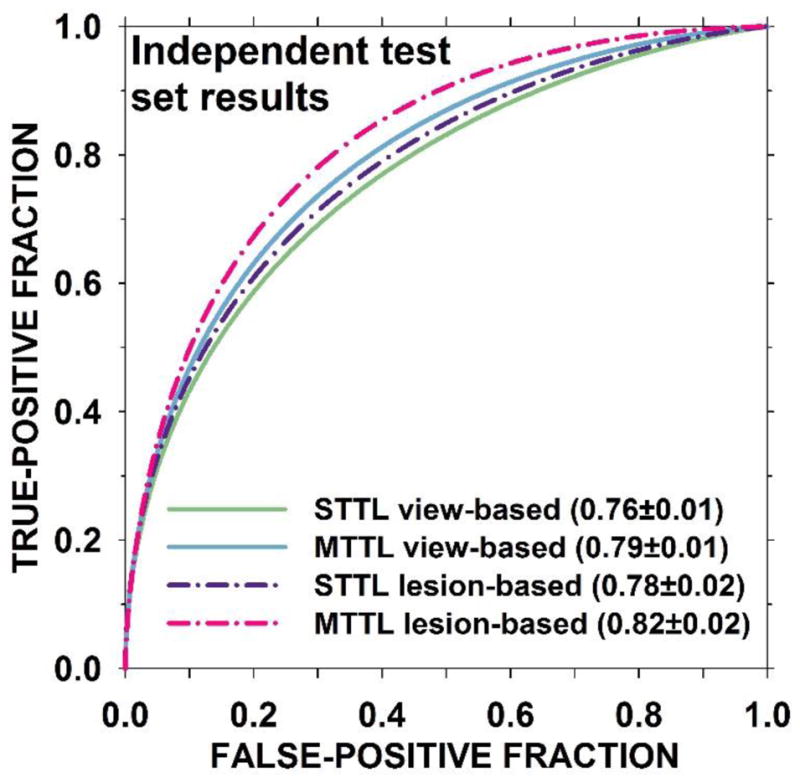
ROC curves for the independent test set using the two selected C1 transfer networks: STTL: single-task transfer learning, MTTL: multi-task transfer learning. The difference in the AUCs was statistically significant between the two lesion-based curves (p-value = 0.007) and between the two view-based curves (p-value = 0.008).
Fig. 7.


Features maps from the deconvolutional network to visualize the features of DCNN trained on mammography data when projected back to the input image. Six feature maps were selected for each convolutional layer. The corresponding feature maps for the malignant (M) and benign (B) mass are shown in the upper and lower rows in each layer.
4. DISCUSSION
We conducted studies to reduce biases among the folds in the N-fold cross-validation, assess different transfer networks for effective knowledge transfer of generic features from non-medical images to medical images, append the additional heterogeneous data by taking advantage of multi-task learning to boost the classification performance, and verify the process with an independent test set. This work provides a deeper understanding of DCNN transfer learning, examines the variabilities in different steps of the process and robustness of the observed results, and demonstrates the potential of multi-task learning to improve the generalizability.
We split the training data randomly by case 10 times for the 4-fold cross-validation to evaluate the dependence of the performance of the trained DCNN on the training subsets. As smaller variations and higher average AUC on the validation folds indicate that the characteristics of the cases among the partitions are more uniform, i.e., the training set (any combination of three of the folds) is more representative of the “population (validation set)” to which the trained DCNN will be applied. Although the 10-time splitting was only a small number among the infinite possibilities and it most likely did not include the optimum, the process illustrated how we selected a more balanced splitting (N2 in fig. 3) for the subsequent analyses.
For all the transfer networks, the convolution layers were copied from the ImageNet trained DCNN while the fully connected layers are randomly initialized. Transfer learning by freezing the first convolution layer alone (C1) provided the best training as shown in fig. 4. With the C0 transfer network, where all the convolutional layers were re-trained with mammography data, the variation of the four fold AUCs was higher than all other transfer networks.
In our previous work on computer-aided detection of masses in digital breast tomosynthesis (DBT), we showed that when a DCNN trained on true positive (TP) and false positive (FP) mass ROIs from SFM and DM was tested directly on ROIs from DBT without any transfer learning, it obtained an AUC of 0.81.(Samala et al., 2016) This result motivated us that similarities between mass representation using different mammography modalities can be exploited to append data sets for DCNN training. Through multi-task transfer learning, the DCNN can learn intermediate representations that are shared across tasks, thereby increasing the feature representation and resulting in improved performance. Fig. 6 shows that the independent test AUC for single- and multi-task transfer learning reached 0.78±0.02 and 0.82±0.02, respectively, for lesion-based performance and 0.76±0.01 and 0.79±0.01, respectively, for view-based performance. The AUC difference between the two methods for lesion-based performance is statistically significant (p-value=0.007). Fig. 8 shows the misclassified ROIs, the top row are biopsy-proven benign lesions and the bottom row are biopsy-proven malignant lesions.
Fig. 8.

Misclassified ROIs from the independent test set. Top row lesions are biopsy-proven benign and bottom row lesions are biopsy-proven malignant. Each ROI is 128 x 128 pixels in size.
We used the t-SNE technique to reduce the feature space from as large as 4096 to 100 dimensions to a two-dimensional map as shown in fig. 5. The t-SNE embedding maps reveal some interesting properties regarding the DCNN features for different transfer networks and across heterogeneous data: (a) From the multi-task embedding, the features for each class (malignant or benign) from each type of images (SFM, DM, DDSM) clustered closely but were relatively separated from the other types, indicating the three types of images have different characteristics. (b) The clusters of the same class from the three types of images moved closer and closer as they were extracted further along the fully connected layers, indicating that the features converged for the more specific malignant and benign classification task, regardless of the image type. (c) The converging trend of the three types of image features indicates that the wider feature representation from the multi-task approach regularized the DCNN training to accommodate variations in the input images, potentially contributing to the generalizability of the DCNN for the mass classification task. The independent test results in fig. 6 reveal a boost in the discriminatory power with the multi-task transfer learning. (d) Considering that the t-SNE maps are rotation-invariant, the shape and separation for the malignant and benign classes of the SFM set on the maps between the single- and multi-task are relatively similar at all fully connected layers. (e) While the features from the SFM and DDSM cases show differences, they are closer to each other than to the DM cases, suggesting the differences between the digitized screen-film and digital image acquisition systems.
The feature maps visualized with the deconvolutional network from the trained DCNN in the mass classification process is shown in fig. 7. The feature maps from the malignant and benign mass examples indicate that: (a) the features extracted between the first and the last convolutional layer vary from generic to more specific as the layer goes deeper, (b) the mass spiculations are highlighted in the malignant mass while the lesion boundary is enhanced in the benign mass, and (c) the image pattern in the region surrounding the malignant mass appears to be more complex than that surrounding the benign mass in most of the feature maps.
There are limitations in this study. First, we did not compare different combinations of layers, nodes and hyperparameters in the DCNN structure. Because of the numerous combinations that can be studied, the computation time and resource are prohibitive at this time. However, our study has demonstrated the potential of multi-task transfer learning that it may be a useful approach for improving the generalizability of the trained DCNN when the data for a given task are limited while data from other related tasks are available. Second, we chose to use ImageNet in this study, it is not known if other DCNNs such as VGG, GoogLeNet may exhibit similar flexibility in multi-task transfer learning. The evaluation of other larger DCNN structures will require larger data sets for transfer learning using either the single-task or multi-task approaches. Third, we did not compare the performance from the DCNN with those from conventional machine learning techniques consisting of feature extraction, feature selection and classification steps because our focus of this study was to study the DCNN training process. Such comparative studies are of interest and will be pursued in the future. Fourth, our DM data set was small so that we could only use SFM as an independent test set. In addition, the DM set was collected with a single vendor DM system. Nevertheless, our study with the available data sets has accomplished the purpose of demonstrating the potential of multi-task transfer learning in medical imaging. We plan to extend the study to include DMs from different vendors as additional tasks and further compare the test performances on DM sets when such data sets become available.
5. CONCLUSION
A multi-task transfer learning DCNN was formulated to translate the ‘knowledge’ learned from non-medical images to medical diagnostic tasks through supervised training and to increase the generalization capabilities of DCNNs by simultaneously learning auxiliary tasks. We compared the multitask approach to traditional single-task transfer learning method for classification of malignant and benign masses in mammography. With transfer learning for DCNNs, multi-task supervised learning achieved better generalization to unknown cases than single-task learning. The proposed multi-task transfer learning DCNN framework shows the strong potential that the lesion classification task in mammography can be extended to similar task in digital breast tomosynthesis while utilizing auxiliary tasks from large SFM and DM data sets.
Acknowledgments
This work is supported by the National Institutes of Health award number RO1 CA151443.
References
- Argyriou A, Evgeniou T, Pontil M. Multi-task feature learning. Advances in neural information processing systems. 2007;19:41. [PMC free article] [PubMed] [Google Scholar]
- Bengio Y. Neural networks: Tricks of the trade. Springer; 2012. pp. 437–78. [Google Scholar]
- Burgess AE. On the noise variance of a digital mammography system. Medical Physics. 2004;31:1987–95. doi: 10.1118/1.1758791. [DOI] [PubMed] [Google Scholar]
- Caruana R. Multitask learning: Learning to learn. Springer; US: 1998. pp. 95–133. [Google Scholar]
- Chan H-P, Wei D, Helvie MA, Sahiner B, Adler DD, Goodsitt MM, Petrick N. Computer-aided classification of mammographic masses and normal tissue: Linear discriminant analysis in texture feature space. Physics in Medicine and Biology. 1995;40:857–76. doi: 10.1088/0031-9155/40/5/010. [DOI] [PubMed] [Google Scholar]
- Chan H-P, Lo SC, Helvie M, Goodsitt MM, Cheng SNC, Adler DD. Recognition of mammographic microcalcifications with artificial neural network. Radiology. 1993;189:318. [Google Scholar]
- Chan H-P, Lo SCB, Sahiner B, Lam KL, Helvie MA. Computer-aided detection of mammographic microcalcifications: Pattern recognition with an artificial neural network. Medical Physics. 1995;22:1555–67. doi: 10.1118/1.597428. [DOI] [PubMed] [Google Scholar]
- Chan H-P, Sahiner B, Lo SC, Helvie M, Petrick N, Adler DD, Goodsitt MM. Computer-aided diagnosis in mammography: detection of masses by artificial neural network. Medical Physics. 1994;21:875–6. [Google Scholar]
- Deng L, Yu D. Deep learning: methods and applications. Foundations and Trends® in Signal Processing. 2014;7:197–387. [Google Scholar]
- Fernando C, Banarse D, Blundell C, Zwols Y, Ha D, Rusu AA, Pritzel A, Wierstra D. Pathnet: Evolution channels gradient descent in super neural networks. 2017 arXiv:1701.08734. [Google Scholar]
- He K, Zhang X, Ren S, Sun J. Deep residual learning for image recognition. Proceedings of the IEEE Conference on Computer Vision and Pattern Recognition; 2016. pp. 770–8. [Google Scholar]
- Heath M, Bowyer K, Kopans D, Moore R, Kegelmeyer P. In: Digital Mammography; IWDM 2000. Yaffe MJ, editor. Toronto, Canada: Medical Physics Publishing; 2001. pp. 457–60. [Google Scholar]
- Intrator N, Edelman S. Learning to learn. Springer; 1996. pp. 135–57. [Google Scholar]
- Krizhevsky A, Sutskever I, Hinton GE. Imagenet classification with deep convolutional neural networks. Advances in neural information processing systems. 2012:1097–105. [Google Scholar]
- Litjens G, Kooi T, Bejnordi BE, Setio AAA, Ciompi F, Ghafoorian M, van der Laak JAWM, van Ginneken B, Sánchez CI. A survey on deep learning in medical image analysis. Medical Image Analysis. 2017;42:60–88. doi: 10.1016/j.media.2017.07.005. [DOI] [PubMed] [Google Scholar]
- Maaten Lvd, Hinton G. Visualizing data using t-SNE. Journal of Machine Learning Research. 2008;9:2579–605. [Google Scholar]
- Metz CE, Pan X. “Proper” binormal ROC curves: Theory and maximum-likelihood estimation. Journal of Mathematical Psychology. 1999;43:1–33. doi: 10.1006/jmps.1998.1218. [DOI] [PubMed] [Google Scholar]
- Pan SJ, Yang Q. A survey on transfer learning. IEEE Transactions on knowledge and data engineering. 2010;22:1345–59. [Google Scholar]
- Sahiner B, Chan H-P, Petrick N, Wei D, Helvie MA, Adler DD, Goodsitt MM. Classification of mass and normal breast tissue: a convolution neural network classifier with spatial domain and texture images. IEEE Transactions on Medical Imaging. 1996;15:598–610. doi: 10.1109/42.538937. [DOI] [PubMed] [Google Scholar]
- Samala RK, Chan H-P, Hadjiiski L, Helvie MA, Wei J, Cha K. Mass Detection in Digital Breast Tomosynthesis: Deep Convolutional Neural Network with Transfer Learning from Mammography. Medical Physics. 2016;43:6654–66. doi: 10.1118/1.4967345. [DOI] [PMC free article] [PubMed] [Google Scholar]
- Shin H-C, Roth HR, Gao M, Lu L, Xu Z, Nogues I, Yao J, Mollura D, Summers RM. Deep Convolutional Neural Networks for Computer-Aided Detection: CNN Architectures, Dataset Characteristics and Transfer Learning. IEEE Transactions on Medical Imaging. 2016;35:1285–98. doi: 10.1109/TMI.2016.2528162. [DOI] [PMC free article] [PubMed] [Google Scholar]
- Simonyan K, Zisserman A. Very deep convolutional networks for large-scale image recognition. 2014 arXiv:1409.1556. [Google Scholar]
- Szegedy C, Liu W, Jia Y, Sermanet P, Reed S, Anguelov D, Erhan D, Vanhoucke V, Rabinovich A. Going deeper with convolutions. Proceedings of the IEEE Conference on Computer Vision and Pattern Recognition; 2015. pp. 1–9. [Google Scholar]
- Tajbakhsh N, Shin JY, Gurudu SR, Hurst RT, Kendall CB, Gotway MB, Liang J. Convolutional Neural Networks for Medical Image Analysis: Full Training or Fine Tuning? IEEE Transactions on Medical Imaging. 2016;35:1299–312. doi: 10.1109/TMI.2016.2535302. [DOI] [PubMed] [Google Scholar]
- Torrey L, Shavlik J. Transfer learning. Handbook of Research on Machine Learning Applications and Trends: Algorithms, Methods, and Techniques. 2009;1:242. [Google Scholar]
- Yosinski J, Clune J, Bengio Y, Lipson H. How transferable are features in deep neural networks? Advances in Neural Information Processing Systems. 2014:3320–8. [Google Scholar]
- Zeiler MD, Fergus R. Visualizing and understanding convolutional networks. European conference on computer vision. 2014:818–33. [Google Scholar]