

Abstract
Motivation
Genomics features with similar genome-wide distributions are generally hypothesized to be functionally related, for example, colocalization of histones and transcription start sites indicate chromatin regulation of transcription factor activity. Therefore, statistical algorithms to perform spatial, genome-wide correlation among genomic features are required.
Results
Here, we propose a method, StereoGene, that rapidly estimates genome-wide correlation among pairs of genomic features. These features may represent high-throughput data mapped to reference genome or sets of genomic annotations in that reference genome. StereoGene enables correlation of continuous data directly, avoiding the data binarization and subsequent data loss. Correlations are computed among neighboring genomic positions using kernel correlation. Representing the correlation as a function of the genome position, StereoGene outputs the local correlation track as part of the analysis. StereoGene also accounts for confounders such as input DNA by partial correlation. We apply our method to numerous comparisons of ChIP-Seq datasets from the Human Epigenome Atlas and FANTOM CAGE to demonstrate its wide applicability. We observe the changes in the correlation between epigenomic features across developmental trajectories of several tissue types consistent with known biology and find a novel spatial correlation of CAGE clusters with donor splice sites and with poly(A) sites. These analyses provide examples for the broad applicability of StereoGene for regulatory genomics.
Availability and implementation
The StereoGene C ++ source code, program documentation, Galaxy integration scripts and examples are available from the project homepage http://stereogene.bioinf.fbb.msu.ru/
Supplementary information
Supplementary data are available at Bioinformatics online.
1 Introduction
Modern high-throughput genomic methods generate large amounts of data, which can come from experimental designs that compare tissue-specific or developmental stage-specific phenomena.
An important challenge of genome-wide data analysis is to reveal and assess the interactions between biological processes, e.g. chromatin profiles and gene expression. An emerging approach to this challenge is to represent the biological data as functions of genomic positions (we use terms profile or track for the functions) and to estimate correlations between these functions.
In recent years, the bioinformatics community has actively developed methods for assessment of colocalization of genomic features (Chikina and Troyanskaya, 2012; Favorov et al., 2012; Kravatsky et al., 2015; Schäfer et al., 2012; Zhang et al., 2011). The features are typically represented as a set of intervals on the genome (genes, repeats, CpG islands, etc.), as point profiles (binding sites, TSS, splice sites) or as continuous (numeric) profiles (coverage of expression, ChIP, etc. from high-throughput sequencing experiments). A common approach to investigating genomic features is to represent these features as intervals, computed from the original continuous coverage data using a threshold or more sophisticated algorithms (Zhang et al., 2008). The tracks resulting from this discretization are sensitive to algorithm parameters, including thresholds and therefore are unable to account different levels of genomic coverage or gene usage.
In addition, most genome-wide correlation algorithms (Kravatsky et al., 2015; Zhang et al., 2011) compare genomic features at identical genomic coordinates (called overlapping coordinates). However, biologically regulatory relationships may often occur between features within a neighborhood of genomic coordinates (called adjacent coordinates). For example, gene expression profiles (RNA-seq coverage) correlate with transcription factor binding sites or chromatin state in nearby promoter regions or distant enhancer regions. Interval and point-based approaches developed for genome-wide correlation account for associations between adjacent coordinates by estimating distance-based statistics (Chikina and Troyanskaya, 2012; Favorov et al., 2012; Kravatsky et al., 2015).
Here, we propose a fast universal method—StereoGene—to correlate numeric genomic profiles. The data can be genome-wide tracks with discrete features (e.g. intervals) or continuous profiles, e.g. coverage data. The method is based on kernel correlation (KC), which provides an estimate of spatially smoothed correlation of two features. The statistical significance of correlations with StereoGene is evaluated by a permutation-based test. StereoGene provides additional functionality, including a track representing correlation as a function of genomic coordinate [called the local correlation (LC)]; calculation of positional cross-correlation function; account for genome-wide confounders by partial correlation. Our implementation is computationally efficient: the calculation of the KC with permutations for a pair of profiles over the human genome takes ∼1–3 min on a personal computer. We demonstrate the effectiveness of StereoGene for estimation of genome-wide epigenetic profile data correlations pairwise correlations between all human samples in the Roadmap Epigenomics Project (Bernstein et al., 2010) dataset and on other open data. These examples describe some potential applications of StereoGene for regulatory genomics to provide a template for its broad utility.
2 Materials and methods
2.1 Kernel correlation
We consider each genomic feature as a numeric function (profile) of the genomic position x. The standard Pearson correlation of two profiles and is defined as:
| (1) |
where is the mean value of f; σf is the SD of f, ; the integration is performed over the genome G. The Pearson correlation relates profile values on exactly the same genomic positions. In biological systems, the relationships of values at proximal but non-overlapping (in genomic coordinates) positions are also important. These correlations may be result from transcriptional regulation, chromatin looping or other interactions. To account for correlations between profiles at proximal coordinates, we generalize the Pearson correlation from Equation (1) to the covariation integral as follows:
| (2) |
where reflects the common sense expectations of the interaction of features at adjacent positions. Formally, it is a function of the distance x − y between the interacting positions. In the case , we get the standard Pearson correlation integral as in Equation (1). In theory, any non-negative kernel function can be used. The default kernel we use is the Gaussian , it is the most intuitive representation of the closer is the position, the more important it is. The σ of the Gaussian reflects the interaction scale and it a user-defined parameter with a reasonable default of 1000 bp.
Based on the Q covariation value (Equation 2), we introduce the KC defined as:
| (3) |
The two-dimensional integral can be rapidly calculated using a complex Fourier transform (Supplementary File S1, Section S1).
| (4) |
where are Fourier coefficients; * means complex conjugate. The value KC(f, g) satisfies the inequality: . The marginal values 1 and −1 correspond to f = g and (see Supplementary File S2, Section S7.3 for the test) Fourier transform can be calculated by the discrete Fast Fourier Transform (FFT) algorithm (Loan, 1992) and therefore has computational cost of where is the length of the genome.
2.2 Cross-correlation
Sometimes, in addition to the overall value of the correlation, an investigator needs information about its local structure, e.g. either the value emerges from a strong position-to-position overlap of it comes from a smooth interaction of neighboring positions and what is the scale of interaction if it exists. To address the questions for our two profiles, f(x) and g(x), StereoGene calculates the cross-correlation function c(x) as follows.
| (5) |
where means the inverse Fourier transform and is elementwise product of fk and vectors of the Fourier coefficients.
2.3 LC profile
The correlation itself shows the similarity of the features at the scale of the genome. The cross-correlation function (see earlier) reflects the fine-scale structure of correlation. The distribution of the correlation as a function of the genomic position is also relevant to determine the nature of interactions. To provide this information, StereoGene generates a new track that describes the local KC of two original profiles as a function of the genomic position, called the ‘LC’.
| (6) |
Note that the value of LC is not restricted by ±1 boundaries and can take any values. The scale of LC depends on the data nature, the direct comparison of LC values makes sense only inside one LC track. To give the user ability to select regions with significant enrichment of LC, StereoGene outputs the FDR LC value (see Section 2.5). Standard peak calling tools (e.g. MACS, Zhang et al., 2008) can be applied to the LC. The result is suitable for gene set enrichment analysis.
2.4 Partial correlation
Non-random correlation of the two profiles may occur due to their correlation with a third profile (confounder) that systematically biases both signals (e.g. level of mapability). An example of such confounding would be the case with ChIP-seq for a sample with the signal from two antibodies (the profiles to correlate) and a common input track (the confounder). StereoGene can computationally exclude such a confounding using the partial correlation (projection) approach. For this calculation, StereoGene correlates the projections both profiles in the subspace, that is orthogonal to the profile a of the confounder as follows:
| (7) |
where (a, f) means a scalar product of the functions a, f. Then, the KC, the LC track, and the cross-correlation between two projection is calculated in a standard way. The statistical significance (see later) is calculated as for a regular two-way comparison.
2.5 Statistical significance
All the calculations we described earlier are executed independently in large (we recommend a size of 100 kb.1M) windows (Fig. 1). This approach allows the FFT to be really fast and at the same time, it provides us with the statistical significance of all the observations. We apply a permutation test to obtain significance for the computed correlation coefficients. Specifically, the correlations (foreground distribution) are calculated in a set of pairs of windows with the same genome positions on the tracks we compare (matched windows). To obtain the null distributions of the values, a shuffling procedure is used that randomly matches windows on one profile to the windows on another profile and then the correlations (background distribution) are computed for these randomly matched window pairs in the same way as they are calculated for the original (matched) window pairs. The statistical significance for KC is provided by a Mann–Whitney test of these two sets of values. The FDR for LC is estimated by using the background distribution as null-hypothesis and the foreground as the signal.
Fig. 1.

The procedure that is used for the estimation of P-values for KC and for the estimation of FDR values for the LC is based on shuffling of windows. Left pane: shuffling procedure. Right pane: background and foreground distributions
2.6 Program implementation
StereoGene is implemented as a command-line tool, and it is distributed as C ++ source code under MIT 2.0 license. StereoGene processes the input data in two passes. On the first pass, StereoGene converts input profiles to an internal binary format and saves the binary profiles for the future runs. The second pass does the Fourier transforms as well as permutations and calculates all the correlations and statistics. If a project refers to a track that has its binary profile already calculated and the parameters have not been changed, StereoGene omits the first pass and reuses the saved profiles. The time required for the first pass depends on the input file size. On a standard computer, for a typical ChIP-Seq track, the first pass takes from a few seconds up to 1–2 min. The second pass takes less than one-half a minute on the human genome.
Input. As input, StereoGene accepts two or more input files in one of the standard genomic tracks formats: BED, WIG, BedGraph and BroadPeak. If more that two track files are provided, StereoGene makes all the pairwise comparisons. StereoGene can take a linear model, which combines a number of profiles to get one of the tracks to compare, as an input. For a batch processing, StereoGene accepts a text file containing a list of the tracks. A linear combination of input tracks (model) described by a text file can be used instead of a track.
Output. StereoGene reports the KC over all the genome; KC values for matched and for shuffled windows, averaged KC over the matched windows and P-value. StereoGene produces the following files: the foreground and background distributions for KC; the cross-correlation function; the LC track; table of FDR values for the LC values and some additional files. The information can be presented on the whole genome as well as by chromosomes.
StereoGene command-line run. The only parameter that does not have a default value and thus is required for a run is a file with the chromosome names and lengths. For the partial correlation, the confounder track should be defined. All other parameters are optional and have reasonable defaults. The less technical of them are the window size and the kernel width. Detailed information about input and output files and parameters is presented in the program documentation at the StereoGene homepage http://stereogene.bioinf.fbb.msu.ru/. The homepage also contains an archive with the example run scripts along with all the necessary files. A general program description is presented in the Supplementary File S2.
Visualization and interface. For a quick and intuitive depiction of results, the StereoGene provide an optional mode that prepares an R script, which represents the output in a multipanel plot (Supplementary File S1, Section S2). The first panel displays foreground and background distributions of genomic windows by the KC. If the foreground distribution is shifted to the right of the background distribution, the plot represents the positive correlation and the left shift shows anticorrelation. The significance of the observation is represented by the Mann–Whitney test that is described in Section 2.5. The second panel, which is the cross-correlation function, represents spatial relationships between the tracks. The third panel represents the LC distribution for the observed (foreground) and the null (background) LC distributions and the FDR q-values. We provide two tool definition files to use StereoGene in Galaxy (Afgan et al., 2016): one to compute and to visualize the correlation of a pair of tracks and another to compute and to visualize the partial correlation given a confounding track.
2.7 Gene set analysis by the LC track
To detect the gene sets that are overrepresented around the areas of high LC of a pair of tracks, we do the following. We take the LC track (*.wig StereoGene output file) convert the track to the BED format using bedops software, version 2.4.16 (Neph et al., 2012) and selected 3000 of the highest peaks using MACS-1.4.2 (Zhang et al., 2008) with the default parameters. Next, we select the genes whose transcription start sites fell within 5 kb of the correlation peak. The resulting list of genes is mined for biological enrichment using DAVID 6.7 software (Huang da et al., 2009). Eventually, we obtain a list of gene-related terms (gene sets), that are significantly overrepresented around the high LC regions, with some statistical measures (adjusted P-value, FDR) for each term.
2.8 Data source
Data from the Roadmap Epigenomics Project (Bernstein et al., 2010) are downloaded from the Human Epigenome Atlas (http://www.genboree.org/). Data for FANTOM4 CAGE clusters (Ravasi et al., 2010) are obtained from the UCSC website (RIKEN CAGE tracks, GEO accession IDs are GSM849326 for nucleus GSM849356 for cytosol in H1 human embryonic stem cell line, RRID:CVCL_9771). The datasets with the tracks are listed in Supplementary File S1, Section S10.
3 Results
StereoGene enables a variety of genome-wide correlation techniques to account for different types of interrelationships between pairs of continuous genomic features. We summarize the major types of correlations enabled by StereoGene in Table 1.
Table 1.
Types of correlations produced by StereoGene
| Type of correlation | Eq. | Description |
|---|---|---|
| KC | (3) | The genome-wide correlation coefficient, which is calculated with the kernel; it reflects overall relationship between two tracks. |
| Cross-correlation | (5) | The cross-correlation function shows the structure of the correlation that reflects distance dependence of the tracks values. |
| LC | (6) | This output track shows the KC as a function of the genome position. The track can be displayed in genome browsers and it can used in further analysis. |
| Partial correlation | (7) | The correlation computed between a pair of profiles, excluding the impact of a third confounding genomic track. |
3.1 StereoGene application examples
3.2 Human Epigenome Atlas pairwise correlation anthology
To demonstrate the wide-range of applications of StereoGene, we have built a pipeline that applies StereoGene to the Human Epigenome Atlas in the Roadmap Epigenomics Project (Bernstein et al., 2010). This database is comprehensive, containing 2423 different data types for 186 different tissues (263 077 pairs total). For our analysis, we correlate data from all pairs of data types in the same tissue (or cell line), and we correlate all pairs of tissues and cell lines from the same data type. All the results are available from http://stereogene.bioinf.fbb.msu.ru/epiatlas.html. Although this database is large, StereoGene compute the correlations efficiently (30 s per each comparison). Therefore, the algorithm well-suited to query intersample correlations in large databases. In addition to testing the computational efficiency of StereoGene on large databases, the comprehensive analysis enables us to compare the StereoGene findings to well-established biological associations.
Genome-wide KC analysis. We first use StereoGene to assess the correlation between distinct epigenetic tracks from the same tissue type. We focus this part of the analysis on pairwise correlations between the most frequently studied tracks in the Roadmap Epigenomics Project, namely, H3K4me1, H3K4me3, H3K9me3, H3K27me3, H3K36me3 epigenetic features and the RNA-seq and on comparisons of the distributions of the KC values for the same epigenetic tracks across fetal and across adult tissues. The distributions of the correlations are presented separately for fetal tissues and for adult tissues (Fig. 2A, Supplementary File S1, Section S10). Generally, the epigenetics marks are more correlated in adult tissues in comparison with the fetal tissues. The statistical significance of this observation is shown on Figure 2B. The highest difference of feature-to-feature correlation between the collections is observed for the H3K9me3 versus H3K27me3 pair: they are significantly more correlated in adult tissues than in fetal ones. A comparison of correlation between H3K9me3 and H3K27me3 in the same tissue for fetal and adult gave a (Wilcoxon test). This result is consistent with the prior observation that at early stages, different genomic regions are separately regulated by H3K9me3 and H3K27me3, but during tissue maturation, these heterochromatin marks became more synchronized (Chen and Dent, 2014). One possible explanation is that H3K27me3 initiates chromatin compaction by recruitment of H3K9me3. The colocalization of H3K27me3 versus H3K36me3 relates to the monoallelic gene expression (Nag et al., 2013). Figure 2 also shows a significant increase of correlation of these marks in adult tissues in comparison with fetal tissues. The observation is consistent with the recent studies (Nag et al., 2015).
Fig. 2.
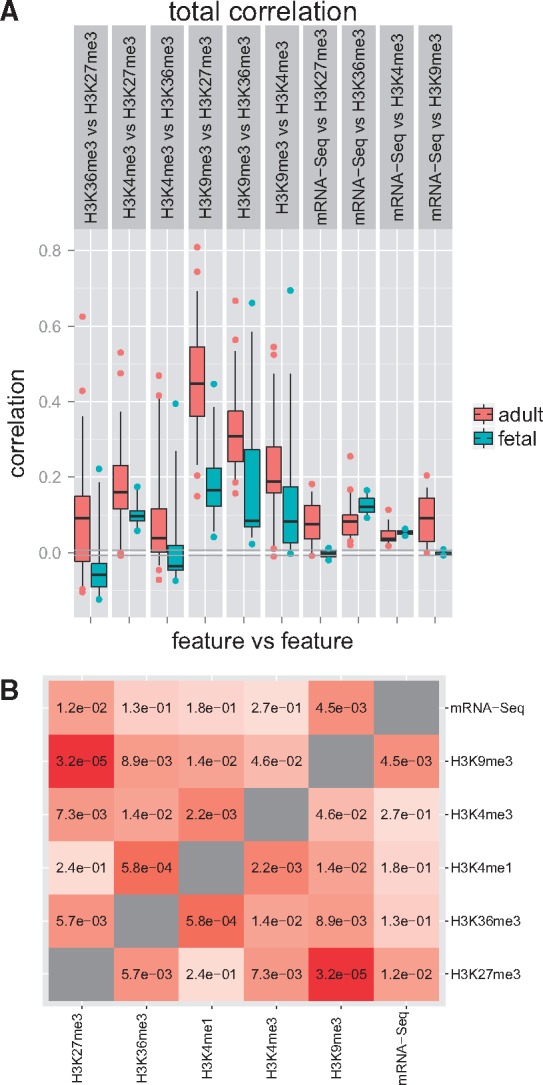
Distributions of genome-wide KCs values of pairs of epigenetic marks across the fetal and across the adult tissues. Twelve fetal and 39 adult cell types data are used. (A) Boxplots of the KC value distribution for adult and fetal tissues. Gray horizontal lines near the zero show the maximal and the minimal background correlations that are observed over all the datasets. (B) P-values for difference of these correlation distributions between fetal and adult tissues (Wilcoxon test)
KC windows distribution. To look at the KC difference between adult and fetal tissues in more details, we compare the H3K4me3 and H3K27me3 KC distributions over the windows of the genome in the adult lung tissue, fetal lung tissue and their common background (Fig. 3A). In this analysis, we observe a higher correlation between H3Kme4 and H3K27me3 in adult in than fetal tissues. This observation is consistent with chromatin changes during development. Specifically, adult tissues have more regions with ‘poised promoters’ in which both marks are active than do fetal tissues (Sachs et al., 2013).
Fig. 3.

Distributions of correlations. (A) H3K27me3 versus H3K4me3 in lung tissues. Solid black line—adult lung; dotted line—fetal lung; gray—the background distribution that coincides for both cell types. (B) Correlation distribution for H3K27me3 versus H3K4me3 in female adult lung cells with chromosome specification. Gray—background distribution; solid line—correlation distribution over genome; dashed—correlation distribution for Chromosome 19, dotted line—correlations for X-chromosome
LC analysis. StereoGene enables positional interpretation of the correlation results providing the LC functionality (see Section 2). Here, we analyze the LC track between the data for H3K4me3 and H3K27me3 marks in adult lung tissue discussed in the previous example. Namely, we compute the LC track to define peaks that define the correlation between these two chromatin marks. We then analyze its function through gene set enrichment analysis (as described in Section 2) of these peaks in resulting LC track (Supplementary File S3). We found that 53 gene sets have FDR ¡5%. In particular, we see the sets ‘cell motion regulation (FDR < )’ and ‘positive regulation of cell migration’ (FDR < ) that are associated with lung development. Specifically, the cell motion is very active during lung development, then it stops in adult lung and its regulation genes are poised, i.e. switched off.
Cross-correlation analysis. Nucleosome dependency of epigenetic marks. As a part of the standard result, StereoGene returns the cross-correlation function between the pairs of samples that were compared. In the Roadmap Epigenomics Project data analysis (see http://stereogene.bioinf.fbb.msu.ru/epiatlas.html), in many cases, we observe the cross-correlation function that has a narrow peak centered at zero. For example, Supplementary Figure S1 shows the distributions of the KC and the cross-correlation function for tracks H3K27me3 versus H3K36me3 in fetal brain cells. Both H3K27me3 and H3K36me3 are covalent histone modifications, they are positioned inside a nucleosome. The zero-peak could reflect frequent cooccurrence of the marks that results from their colocalization inside one nucleosome. This possibility is supported by recent results from reChIP (Kinkley et al., 2016).
Simulations. Nucleosome dependency of epigenetic marks. Widespread application of StereoGene to epigenetic data indicates that positive correlations between histone marks are far more common than negative correlation (Fig. 2) for all histone marks and tissue types. To test whether the pervasive positive correlations has the same nature as the zero-position peak of the cross-correlation function and that they both occur due to the nucleosome positioning, we perform a simulation experiment (Supplementary File S1, Section S8). We simulate a ‘genome’ that is 60 Mbases long and contains 100 000 randomly distributed ‘nucleosomes’. Then we generate two independent signals that are located only on ‘nucleosomes’. As a result, we have obtained simulated data with true positive correlation and with zero peaks. When the signals are produced independently of the ‘nucleosomes’, the peak is not observed and the KC approximately equals to zero. On the other hand, when the simulated signals are colocalized in the simulated nucleosomes we observe a sharp cross-correlation peak at zero. Thus, this simulation suggests that the prevalence of positive KC values and the zero-positioned peak on the cross-correlation observed earlier arise from nucleosome positioning rather than from artifacts.
3.3 Chromosome-specific correlation of the histone modifications
The relation between epigenetic marks can differ from chromosome to chromosome. StereoGene allows to provide the analysis separately by chromosomes. To show this feature, we compared the relationship between two well-investigated histone marks: the promoter-related H3K4me3, and the heterochromatin polycomb-related H3K27me3, in the adult lung, chromosome by chromosome (Fig. 3B). The window KC value distribution for these marks over all genome has a high peak on positive correlations. At the same time, the distribution on Chromosome 19 has a significantly different shape and it is shifted to lower values. This could be explained by the high-gene density, especially, high-housekeeping genes density on the Chromosome 19. The correlation distribution on Chromosome X also differs from the distribution over genome and the Chromosome X distribution has a peak on very high correlations (Fig. 3B), that can be due to the two copies X-chromosome, one is repressed by H3K27me3 mark, while another is active. This observation is consistent with known suppression of Chromosome X in female origin somatic cells as part of development.
3.4 Partial correlations
A pair of features in genome never exist in isolation. Interactions of biological features with other genome-wide features will skew the spatial correlation. For example, differences in mappability of short regions to different regions of the genome will impact the signal of all genome-wide data that requires alignment, and the correlations that can be computed in different regions. The influence of additional and sometimes technical genome-wide features sometimes shadows the effect or can cause an apparent new effect that is unrelated to the biology. We call these additional features that impact correlation of biological features ‘third players’ or ‘confounders’. When the third player genome-wide track is provided, StereoGene uses the partial correlation use-case to eliminate its impact on correlation. Here, we provide examples where using this third track enables StereoGene to both uncover shadowed effects and remove technical associations between unrelated tracks.
The H3K4me3 is an ‘active promoter’ mark and it is expected to be positively correlated with RNA-seq. Indeed, Figure 4A shows some weak positive, though statistically significant correlation in Brain Hippocampus Middle. This tissue is an adult one, and we suppose that a significant share of the promoters is ‘poised’ (Sachs et al., 2013) (see the LC Analysis). In other words, the H3K4me3 effect on the expression is shaded by the H3K27me3 presence. We used the partial correlation mode to remove H3K27me3 influence (Fig. 4B), and the correlation we observe is much stronger. This suggests that the relationship of H3K4me3 to gene expression is modulated by H3K27me3.
Fig. 4.

Distributions of the KC values over the windows: (A) correlation of H3K4me3 versus mRNA-seq in Brain Hippocampus Middle; (B) the same correlation, where the H3K27me3 track is accounted for as a confounder by the partial correlation procedure. (C) KC values distribution for H3K27me3 versus H3K4me3 in GM12878 cells; (D) the same with the nucleosome track accounted for as a confounder. Black line—foreground distribution; gray line—background correlation distribution
As we observed in the cross-correlation analysis, exact nucleosome positioning confounds all the pairwise histone marks. Therefore, correlations between histone marks often occur because of detection near nucleosome coordinates rather than biological similarities between histone marks in the cell. Using a nucleosome track as the confounder for partial correlation in StereoGene decreases the correlation between H3K27me3 and H3K4me3 in GM12878 cells (Fig. 4C and D, Supplementary Fig. S2). Removing the effect of the nucleosome positioning is limited to datasets that contain nucleosome track data, which are regrettably few. More detailed description about the influence of the confounders and their removal with partial correlation functions in StereoGene is presented in the Supplementary File S1, Section S3. Another promising application of the partial correlation to the ChIP-seq data is to exclude the input DNA track as a confounder (Supplementary Fig. S2).
3.5 Cross-correlation function: chromatin marks versus gene features
The local regulation of transcription by chromatin marks usually depends on the positioning of the modified nucleosome relative to the transcription start site. Similar dependence may also occur for other gene features, including gene end sites or exons–introns boundaries. We apply the cross-correlation function in StereoGene to assess the relationship of such gene features to expressed and silenced genes in the brain cingulate gyrus. To compute this correlation, we first define a set of expressed genes as those with the top 25% of mRNA-seq gene values of gene counts and silenced genes as those with gene counts in the bottom 25%. All other genes are called moderately expressed. Then, we plot the cross-correlation function of histone marks versus gene features—start/end and intron beginning/end (Supplementary File S1, Section S4) aggregated for each group of genes. We observe the following.
The distribution of H3K4meX and H3K9ac near TSS of the active genes has two high peaks left and right from TSS and a gap at TSS position. This behavior is in an agreement with other research (Ernst and Kellis, 2015).
Both H3K4meX and H3K9ac density have a sharp break near intron ends. This behavior may be related to epigenomic splice site definition (Brown et al., 2012).
H3K27me3 has a rather narrow peak downstream from TSS of active genes, while for the low-expressed and for the silent genes the peak is wider and it covers TSS. This peak in active genes may be related to a monoallelic expression (Nag et al., 2013).
3.6 DNA-binding proteins: cohesin and histone modifications
One of the promising applications of StereoGene is the analysis of relations of DNA-binding protein with other genomic features. We use the KC from StereoGene to determine the positional correlations of cohesin protein Rad21 ChIP-seq track with CTCF track and with different histone modifications in H1 stem cells (RRID:CVCL_9771) and in the K562 (RRID:CVCL_5145) cell line (Supplementary File S1, Section S5). We observe a very strong positional correlation of the CTCF binding with Rad21 binding (P-value , see Supplementary File S1, Section S5, Table 1). Another observation is that promoter and enhancer marks (H3K4meX) are colocalized with cohesin binding (P-value ), while actively transcribed gene regions and repressed gene regions are not. These observations are consistent with (Steiner et al., 2016) and suggest that StereoGene is a robust tool to associate DNA protein bindings.
3.7 Genome-wide expression: CAGE versus gene annotation
CAGE FANTOM4 (Ravasi et al., 2010) data (CAGE clusters) represents a genome-wide map of capped mRNA. The CAGE data is expected to estimate mRNA that are prevented from degradation and promoted for translation genomewide. As a result, these data are hypothesized to correlate strongly with transcription start sites. To determine whether there is a statistically significant CAGE signal in gene start sites and other gene features, we analyze the positional relationship of CAGE data, for the nucleus and for cytosol of H1-hESC cells with the RefSeq (Pruitt et al., 2009) gene annotations with the StereoGene KC. As hypothesized, CAGE clusters are highly correlated with gene starts. We do not see any signal at the promoter regions but we observe less obvious phenomena, namely, strong positional correlation of CAGE clusters with the intron start sites (donor splice sites) and strong positional correlation of CAGE clusters with transcription termination sites, see Supplementary File S1, Section S6 for more details. CAGE association with intron starts may be explained by the activity of debranching enzymes (Ruskin and Green, 1985). After lariat debranching, the freed end of the intron may become available for capping, and this cap would be detected by CAGE. Indeed, short (18–30 nt) RNAs with the 3′ end that exactly maps to donor splice sites are observed (Taft et al., 2010). The transcriptional termination site correlation is less evident, though it suggests that occasional capping of the free end after cleavage by the polyadenylation complex is possible. The StereoGene analysis of CAGE data enables unprecedented associations of CAGE with gene annotations to assess the function on mRNA capping in different gene features.
3.8 Comparison with other methods
We compare (Table 2) the StereoGene functionality with that of commonly used tools. Notably, very few programs can compute on continuous data and require the establishment of often arbitrary thresholds to create intervals for analysis. KLTepigenome (Madrigal and Krajewski, 2015) is able to work with the continuous profiles but it is limited to sparse data and is quite slow even when being compared to StereoGene doing the same computation on the full profile.
Table 2.
Comparison of functionality for correlation analysis programs
| Program features | IntervalStatsa | BEDToolsb | GenomicRangesc | GenometriCorrd | Genome Track Analyzere | KLTepigemomef | Genomic HyperBrowserg | GATh | StereoGene |
|---|---|---|---|---|---|---|---|---|---|
| Correlate non-local features | + | + | + | + | + | + | − | + | + |
| Interval profiles | + | + | + | + | + | + | + | + | + |
| Work with continuous data | − | − | − | − | − | + | − | − | + |
| Statistical evaluation | + | − | − | + | + | + | + | + | + |
| Partial correlation | − | − | − | − | − | − | − | − | + |
| Stratification by annotation | + | − | − | − | − | − | − | − | − |
| Liquid correlation | − | − | − | − | − | − | − | − | + |
| Produce correlation profile | − | − | − | − | − | − | − | − | + |
| Cross-correlation function | − | − | − | − | − | − | − | − | + |
Lawrence et al. (2013);
Favorov et al. (2012);
Kravatsky et al. (2015);
Sandve et al. (2010);
Heger et al. (2013).
We test consistency of our results with the results, which are described in (Zhou and Troyanskaya, 2014) on modENCODE (Gerstein et al., 2014) S2-DRSC cell line dataset. We find the numeric agreement to be satisfactory. The Pearson correlation coefficient of the KC values and the interaction energy score (Zhou and Troyanskaya, 2014) is 0.48. Our results are summarized and visualized in the Supplementary File S1, Section S7.
4 Discussion
We present a new method, StereoGene, with unprecedented speed for estimation of genome-wide positional correlations. A comprehensive description of the mutual positioning of genome-wide tracks requires a set of statistical test on different scales. For that to happen, StereoGene provides a collection of genome-wide correlation techniques (see Section 3).
We apply the program for a variety of datasets including continuous (ChIP-seq) and interval (genome annotation) data. The results are consistent with recent biology knowledge. In addition, we observe the changes in the correlation between epigenomic features across developmental trajectories of several tissue types, and we find an unexpected strong spatial correlation of CAGE clusters with splicing donor and poly(A) sites. Both observations require verification and both are in concordance with the biological intuition of other authors.
In contrast with other methods in the literature, StereoGene is unique in its ability to rapidly compute correlations of continuous genome-wide features in addition to discrete gene intervals used in most correlation techniques. As seen on public datasets, the approach yields biologically plausible results. The most common application of StereoGene is the association of distinct genomic features from the same individual or common genomic feature between individuals. The correlation distribution plots enable assessment of directionality in addition to statistical significance, to depict multiple varieties in these genome-wide associations. In addition, LC tracks can be used for traditional gene enrichment analysis or to describe the relationship between genomic features. The partial correlation allows excluding of a known confounder. Other features of StereoGene, such as batch analysis and using of linear models, make this tool useful for mass and diverse analysis of the genomic tracks.
As far as we work with the continuous tracks directly, we do not lose information on the binarization approaches as the most methods do. In these other methods, the choice of the binarization threshold is usually supported by reasonable statistical considerations. However, despite the threshold quality, the dependency of the results the threshold should be checked before conclusions of biological associations are drawn with these threshold-based methods. The biological data are obtained on a large population of cells, which can be very inhomogeneous, see, e.g. the phenomenon of gene expression bursts (Bahar Halpern et al., 2015). Thus, even small averaged signals can be biologically significant. We test (Supplementary File S1, Section S9) the dependency of the correlation (KC) value on the binarization threshold. High thresholds lead to overestimated correlations.
Currently, StereoGene is widely applicable for analysis of similarity of genomic–track-represented biological data, including massive analysis. The track-to-track distance results can be aggregated to compare different tissues and different time course points.
Quite often, we observe bimodal KC distribution, and a question whether the modes correspond to some global chromatin states is naturally raised. The first hypothesis we intend to test in this way is a relation to the chromatin A/B compartmentalization (Dekker et al., 2013). The LC track can be compared with some third data source by the next run of StereoGene; the result of the sequential runs is a three-way correlation that is analogous to the liquid correlation (Li et al., 2004). This analysis will enable, particularly, more fine testing of the relations of epigenetic features mutual positioning along the chromosome with the 3D positioning of the chromatin.
We intend to add statistical tests that compare the distributions of observed correlations from different track pairs (e.g. input tracks). It is a natural differential mode without the permutation-based estimations. For the case when the researcher has a collection of tracks for the same tissue, we plan to computationally estimate their common component to use it as a common input track. These new approaches will extend StereoGene beyond robust genome-wide associations to a comprehensive platform for continuous data analysis of genome-wide tracks for cross-platform, integrated genomics analyses.
Supplementary Material
Acknowledgements
The authors are grateful to Roman Kudrin, Ekaterina Khrameeva and Alexandra Galytsyna for testing the program. Thanks to Renat Arufilov, Artur Zalevsky and to Dmitriy Vinogradov for technical solutions and for support. Thanks to Aleksey Stupnikov for his ideas for the future. Thanks to Leslie Cope for his advice. Thanks to Patricia Palmer for her help with the text of the article.
Funding
This work was supported by Russian Science Foundation [grant 14-24-00155]; by National Institutes of Health [grants P30 CA006973, NCI R01CA177669]; by Allegheny Health Network-Johns Hopkins Cancer Research Fund and JHU IDIES/Moore Foundation and by Russian Foundation for Basic Research [grants 14-04-01872, 14-04-00576].
Conflict of Interest: none declared.
References
- Afgan E. et al. (2016) The Galaxy platform for accessible, reproducible and collaborative biomedical analyses: 2016 update. Nucleic Acids Res, 44, W3–W10. [DOI] [PMC free article] [PubMed] [Google Scholar]
- Bahar Halpern K. et al. (2015) Bursty gene expression in the intact mammalian liver. Mol. Cell, 58, 147–156. [DOI] [PMC free article] [PubMed] [Google Scholar]
- Bernstein B.E. et al. (2010) The NIH roadmap epigenomics mapping consortium. Nat. Biotechnol., 28, 1045–1048. [DOI] [PMC free article] [PubMed] [Google Scholar]
- Brown S.J. et al. (2012) Chromatin and epigenetic regulation of pre-mRNA processing. Hum. Mol. Genet., 21, R90–R96. [DOI] [PMC free article] [PubMed] [Google Scholar]
- Chen T., Dent S. (2014) Chromatin modifiers and remodellers: regulators of cellular differentiation. Nat. Rev. Genet., 15, 93–106. [DOI] [PMC free article] [PubMed] [Google Scholar]
- Chikina M., Troyanskaya O. (2012) An effective statistical evaluation of ChIPseq dataset similarity. Bioinformatics, 28, 607–613. [DOI] [PMC free article] [PubMed] [Google Scholar]
- Dekker J. et al. (2013) Exploring the three-dimensional organization of genomes: interpreting chromatin interaction data. Nat. Rev. Genet., 14, 390–403. [DOI] [PMC free article] [PubMed] [Google Scholar]
- Ernst J., Kellis M. (2015) Large-scale imputation of epigenomic datasets for systematic annotation of diverse human tissues. Nat. Biotechnol., 33, 364–376. [DOI] [PMC free article] [PubMed] [Google Scholar]
- Favorov A. et al. (2012) Exploring massive, genome scale datasets with the GenometriCorr package. PLoS Comput. Biol., 8, e1002529–e1002529.. [DOI] [PMC free article] [PubMed] [Google Scholar]
- Gerstein M.B. et al. (2014) Comparative analysis of the transcriptome across distant species. Nature, 512, 445–448. [DOI] [PMC free article] [PubMed] [Google Scholar]
- Heger A. et al. (2013) GAT: a simulation framework for testing the association of genomic intervals. Bioinformatics, 29, 2046–2048. [DOI] [PMC free article] [PubMed] [Google Scholar]
- Huang da W. et al. (2009) Systematic and integrative analysis of large gene lists using DAVID bioinformatics resources. Nat. Protoc., 4, 44–57. [DOI] [PubMed] [Google Scholar]
- Kinkley S. et al. (2016) reChIP-seq reveals widespread bivalency of H3K4me3 and H3K27me3 in CD4(+) memory T cells. Nat. Commun., 7, 12514–12514.. [DOI] [PMC free article] [PubMed] [Google Scholar]
- Kravatsky Y. et al. (2015) Genome-wide study of correlations between genomic features and their relationship with the regulation of gene expression. DNA Res., 22, 109–119. [DOI] [PMC free article] [PubMed] [Google Scholar]
- Lawrence M. et al. (2013) Software for computing and annotating genomic ranges. PLoS Comput. Biol., 9, e1003118. [DOI] [PMC free article] [PubMed] [Google Scholar]
- Li K. et al. (2004) A system for enhancing genome-wide coexpression dynamics study. Proc. Natl. Acad. Sci. USA, 101, 15561–15566. [DOI] [PMC free article] [PubMed] [Google Scholar]
- Loan C.V. (1992) Computational Frameworks for the Fast Fourier Transform. SIAM, Philadelphia, PA. [Google Scholar]
- Madrigal P., Krajewski P. (2015) Uncovering correlated variability in epigenomic datasets using the Karhunen-Loeve transform. BioData Min., 8, 20. [DOI] [PMC free article] [PubMed] [Google Scholar]
- Nag A. et al. (2013) Chromatin signature of widespread monoallelic expression. eLife, 31, e01256.. [DOI] [PMC free article] [PubMed] [Google Scholar]
- Nag A. et al. (2015) Chromatin signature identifies monoallelic gene expression across mammalian cell types. G3, 5, 1713–1720. [DOI] [PMC free article] [PubMed] [Google Scholar]
- Neph S. et al. (2012) BEDOPS: high-performance genomic feature operations. Bioinformatics, 28, 1919–1920. [DOI] [PMC free article] [PubMed] [Google Scholar]
- Pruitt K. et al. (2009) NCBI reference sequences: current status, policy and new initiatives. Nucleic Acids Res., 37(Database issue), D32–D36. [DOI] [PMC free article] [PubMed] [Google Scholar]
- Quinlan A.R., Hall I.M. (2010) BEDTools: a flexible suite of utilities for comparing genomic features. Bioinformatics, 26, 841–842. [DOI] [PMC free article] [PubMed] [Google Scholar]
- Ravasi T. et al. (2010) An atlas of combinatorial transcriptional regulation in mouse and man. Cell, 140, 744–752. [DOI] [PMC free article] [PubMed] [Google Scholar]
- Ruskin B., Green M. (1985) An RNA processing activity that debranches RNA lariats. Science, 229, 135–140. [DOI] [PubMed] [Google Scholar]
- Sachs M. et al. (2013) Bivalent chromatin marks developmental regulatory genes in the mouse embryonic germline in vivo. Cell Rep., 3, 1777–1784. [DOI] [PMC free article] [PubMed] [Google Scholar]
- Sandve G.K. et al. (2010) The genomic HyperBrowser: inferential genomics at the sequence level. Genome Biol., 11, 12.. [DOI] [PMC free article] [PubMed] [Google Scholar]
- Schäfer M. et al. (2012) Integrative analyses for omicsdata: a Bayesian mixture model to assess the concordance of ChIP-ChIP and ChIP-seq measurements. J. Toxicol. Environ. Health A, 75, 461–470. [DOI] [PubMed] [Google Scholar]
- Steiner L. et al. (2016) CTCF and cohesinSA-1 mark active promoters and boundaries of repressive chromatin domains in primary human erythroid cells. PLoS One, 11, e0155378.. [DOI] [PMC free article] [PubMed] [Google Scholar]
- Taft R. et al. (2010) Nuclear-localized tiny RNAs are associated with transcription initiation and splice sites in metazoans. Nat. Struct. Mol. Biol., 17, 1030–1034. [DOI] [PubMed] [Google Scholar]
- Zhang Y. et al. (2008) Model-based analysis of ChIP-seq (MACS). Genome Biol., 9, R137.. [DOI] [PMC free article] [PubMed] [Google Scholar]
- Zhang Y. et al. (2011) QDMR: a quantitative method for identification of differentially methylated regions by entropy. Nucleic Acids Res., 39, e58.. [DOI] [PMC free article] [PubMed] [Google Scholar]
- Zhou J., Troyanskaya O.G. (2014) Global quantitative modeling of chromatin factor interactions. PLoS Comput. Biol., 10, e1003525.. [DOI] [PMC free article] [PubMed] [Google Scholar]
Associated Data
This section collects any data citations, data availability statements, or supplementary materials included in this article.