Abstract
Motivation
Identification of disease-associated miRNAs (disease miRNAs) is critical for understanding disease etiology and pathogenesis. Since miRNAs exert their functions by regulating the expression of their target mRNAs, several methods based on the target genes were proposed to predict disease miRNA candidates. They achieved only limited success as they all suffered from the high false-positive rate of target prediction results. Alternatively, other prediction methods were based on the observation that miRNAs with similar functions tend to be associated with similar diseases and vice versa. The methods exploited the information about miRNAs and diseases, including the functional similarities between miRNAs, the similarities between diseases, and the associations between miRNAs and diseases. However, how to integrate the multiple kinds of information completely and consider the biological characteristic of disease miRNAs is a challenging problem.
Results
We constructed a bilayer network to represent the complex relationships among miRNAs, among diseases and between miRNAs and diseases. We proposed a non-negative matrix factorization based method to rank, so as to predict, the disease miRNA candidates. The method integrated the miRNA functional similarity, the disease similarity and the miRNA-disease associations seamlessly, which exploited the complex relationships within the bilayer network and the consensus relationship between multiple kinds of information. Considering the correlation between the candidates related to various diseases, it predicted their respective candidates for all the diseases simultaneously. In addition, the sparseness characteristic of disease miRNAs was introduced to generate more reliable prediction model that excludes those noisy candidates. The results on 15 common diseases showed a superior performance of the new method for not only well-characterized diseases but also new ones. A detailed case study on breast neoplasms, colorectal neoplasms, lung neoplasms and 32 other diseases demonstrated the ability of the method for discovering potential disease miRNAs.
Availability and implementation
The web service for the new method and the list of predicted candidates for all the diseases are available at http://www.bioinfolab.top.
Supplementary information
Supplementary data are available at Bioinformatics online.
1 Introduction
MicroRNAs (miRNAs) are small non-coding RNAs that regulate the expression of their mRNA targets through RNA cleavage or translational repression (Bartel, 2004; Chatterjee and Grosshans, 2009; He and Hannon, 2004). The dysregulation of miRNAs can cause developmental defects and contributes to progression of various diseases (Calin and Croce, 2006; Meola et al., 2009; Sayed and Abdellatif, 2011). Hence identifying disease-associated miRNAs (disease miRNAs) can provide novel insights into the genetic causes and consequences of complex diseases.
Aided by large scale deep sequencing, computational prediction of disease miRNAs can provide reliable miRNA candidates for further functional analysis in disease studies. Several methods have been developed for predicting disease miRNAs, which fall into two main categories. The methods in the first group extensively exploited the negative regulation of miRNAs on their target mRNAs (Bartel, 2004). They first identified the sets of target genes based on the complementarity between miRNA sequences and the sequences of putative target genes. The disease miRNA candidates were then inferred according to the similarities or the interactions between the target genes and the known disease-related genes (Jiang et al., 2010; Li et al., 2011; Shi et al., 2013). However, the experimentally validated target genes are so scanty that they fail to support the methods effectively. Hence the target prediction programs, such as TargetScan (Lewis et al., 2003) and PITA (Kertesz et al., 2007), have been adopted to obtain the majority of target genes. Due to the high false positive rate of target prediction results (Bartel, 2009; Liu et al., 2014; Ritchie et al., 2009), it is difficult for the methods of the first group to achieve excellent prediction accuracy.
In the second category, as functionally related miRNAs are usually involved in similar diseases (Bandyopadhyay, 2010; Goh et al., 2007; Lu et al., 2008), the functional similarity of two miRNAs was measured based on their associated diseases successfully (Wang et al., 2010). A functional similarity network of miRNAs was further constructed and denoted as MiRNet. Several methods were proposed to prioritize the miRNA candidates for a specific disease (Chen, 2012; Xuan et al., 2015) via random walks on MiRNet. Similarly, Chen’s method inferred the disease candidates related to a specific miRNA via random walks on the disease network (Chen and Zhang, 2013). HDMP exploited the k most similar neighbors and the distribution of known disease miRNAs to infer the miRNA candidates (Xuan et al., 2013). These methods relied on a seed set of miRNAs that have already been related to the specific disease and therefore are not effective on the new diseases without any known related miRNAs. Recently, the information about diseases was introduced into the prediction methods to make them applicable to all the diseases, especially to the new ones (Chen and Yan, 2014; Liu et al., 2016; Xuan et al., 2015). However, Chen et al. established the separate objective functions for the miRNA network and the disease network respectively, which did not integrate the multiple kinds of information about miRNAs and diseases completely. Xuan et al. and Liu et al. concentrated on the prediction for the single disease and ignored the correlation between the candidates related to different diseases.
We propose and develop a novel prediction method based on non-negative matrix factorization and refer to it as DMPred. DMPred focuses on the following three important aspects. First, it is well known that miRNAs with similar functions tend to be associated with similar diseases and vice versa. As a result, the miRNA functional similarity, the disease similarity and the miRNA-disease associations are consistent with each other. Considering the consensus relationship, DMPred integrates the multiple kinds of information about miRNAs and diseases seamlessly. Second, in terms of two similar diseases, their associated miRNA candidates are correlated rather than independent. Hence DMPred predicts their respective candidates for all the diseases simultaneously instead of for a single disease. Third, as only a small number of miRNAs are relevant to a specific disease (Kosik, 2006; Shi et al., 2013), the predicted associations between miRNAs and diseases should be sparse. DMPred takes the sparseness characteristic into account, which contributes to the generation of more reliable prediction model that excludes the noisy candidates.
2 Materials and methods
Our goal is to develop a global method that is able to simultaneously predict their respective associated miRNA candidates for all the diseases. We first constructed a bilayer network of miRNAs and diseases to represent the complex relationships between them. A novel prediction method based on non-negative matrix factorization with sparseness constraints was proposed specifically for the network.
Let S be the set that contains all the diseases. For a specific disease , the known d-related miRNAs are referred to as the labeled nodes, and the remaining miRNAs which have no information of relevance to d, are the unlabeled nodes. As the unlabeled nodes may potentially be associated with d, we correlate an unlabeled node ui with an association score . The higher , the more ui is likely to be associated with d. All the unlabeled nodes are ranked by their scores and the top ranked nodes are regarded as the promising d-related candidates.
2.1 Disease similarity measurement
The disease similarity quantifies how similar they are from the perspectives of disease semantics and symptom. The similarity of two diseases are calculated based on their common semantic annotations and shared disease symptoms.
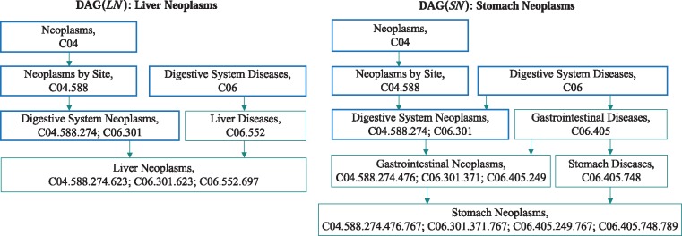
Disease semantic similarity. We calculated the semantic similarity between diseases by using the existing measurement (Wang et al., 2010). Each disease is represented with a directed acyclic graph (DAG) which contains all the annotation terms related to the disease. Figure 1 shows the DAGs of two diseases ‘Liver Neoplasms (LN)’ and ‘Stomach Neoplasms (SN)’. The DAG of a disease like LN is denoted as DAG(LN) = (TLN, ELN), where TLN is a set that includes all the ancestor nodes of LN and LN node itself, and ELN is a set of edges connecting these nodes. Each node t () has its semantic contribution, which is calculated by
| (1) |
where is an semantic contribution adjustment factor for the edges linking node t with its child . As suggested in the literature (Wang et al., 2010), it is set to 0.5. The overall semantic value of disease LN, DV(LN), is defined as
| (2) |
As two diseases sharing more terms in their DAGs are more similar, the semantic similarity between two diseases LN and SN is defined as
| (3) |
where and are the semantic values of term t related to diseases LN and SN, respectively. The semantic similarity of two diseases ranges between 0 and 1.
Fig. 1.
The DAGs of the diseases Liver Neoplasms and Stomach Neoplasms. Each node contains one disease term and its identification numbers. The blue bold nodes are the common terms of these two diseases (Color version of this figure is available at Bioinformatics online.)
Disease phenotypic similarity. It is well studied that two diseases sharing more common phenotypes (signs and symptoms) are often more similar. Hoehndorf et al. (2015) measured the phenotypic similarities between diseases by integrating the phenotype data from the OMIM database (Hamosh et al., 2005) and the Orphanet database (Weinreich et al., 2008) and the phenotype ontology information. The phenotypic similarity of two diseases also ranges between 0 and 1.
Integrating disease semantic and phenotypic similarity. Let PS(A, B) be the phenotypic similarity between two diseases A and B. In order to incorporate their semantic and phenotypic similarities, the similarity of A and B, DS(A, B), is defined as follows,
| (4) |
where is a trade-off parameter determining the importance of the semantic similarity and it is set to 0.5 in our experiments. The values of the disease similarity range between 0 and 1.
2.2 MiRNA similarity measurement
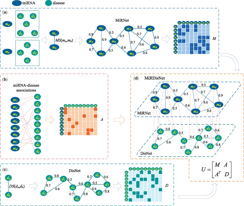
The functional similarity of two miRNAs quantifies how similar their functions are. Based on the observation that miRNAs with similar functions are usually implicated in similar diseases, Wang et al. estimated the functional similarity of two miRNAs by measuring the similarity between their associated two groups of diseases (Wang et al., 2010). Consider Figure 2a as an example, miRNA ma is associated with diseases d1, d2, d3, d4 and d8, and mb is associated with d1, d2, d5 and d8. The similarity between and is calculated as the functional similarity of ma and mb and denoted as .
Fig. 2.
Construction of a miRNA-disease bilayer network and its matrix representation. (a) Calculate the functional similarity of two miRNAs based on their associated diseases and construct a miRNA network (MiRNet) and its adjacent matrix M. (b) Construct an adjacent matrix A according to the known miRNA-disease associations. (c) Calculate the similarity of two diseases based on their common semantic annotations and shared symptoms, and construct a disease network (DisNet) and its adjacency matrix D. (d) Construct the miRNA-disease bilayer network (MirDisNet) and its adjacent matrix U
The miRNA similarity is calculated by using Wang’s measurement method. We firstly compute the similarity between a disease, such as d1, and a group of diseases, such as DTb. It is defined as follows,
| (5) |
where . The similarity of two miRNAs, such as ma and mb, is obtained by calculating the similarity of DTa and DTb. It is defined as,
| (6) |
where and is the numbers of diseases in DTa and DTb respectively. is the similarity between and the disease group DTb, and is the similarity between and DTa. The similarity of two miRNAs also ranges between 0 and 1.
2.3 Construction of miRNA-disease bilayer network
We construct a miRNA-disease bilayer network which contains two kinds of nodes (miRNAs and diseases) and three types of relationships (miRNA-miRNA similarity relationship and disease-disease similarity relationship, as well as miRNA-disease association relationship). The bilayer network is composed of a miRNA functional network, a disease network and the edges connecting the two networks. Figure 2 demonstrates the workflow of constructing the network and its matrix representation.
Construction of MiRNet. The miRNA functional network (MiRNet) is constructed by connecting any two miRNAs whose functional similarity is more than 0. The topology structure of MiRNet and the functional similarities between miRNAs are captured by a weighted graph . Each vertex represents a miRNA, and an edge connects two vertices indicating there is a functional link between them. The weight of em quantifies the functional similarity degree of these two vertices. Let be an adjacency matrix of GM. Nm is the number of miRNAs, denotes the set of real numbers, and represents real coordinate space of dimensions. Mij is defined as follows,
| (7) |
where is the functional similarity of mi and mj. Obviously, M is a symmetric matrix.
Construction of DisNet. In terms of the disease network (DisNet), its topology structure and the similarities between diseases are denoted by a weighted graph (Fig. 2c). Each vertex represents a disease, and an edge captures the relation between two diseases. The weight wd of edge ed quantifies how similar two diseases are. Two disease nodes in DisNet are connected if their similarity is greater than 0. Let be an adjacency matrix of GD. Nd is the number of diseases, and Dij is defined as follows,
| (8) |
where is the similarity of the diseases di and dj. D is also a symmetric matrix.
Edges between MiRNet and DisNet. If a miRNA within MiRNet has been experimentally validated to be associated with a disease within DisNet, an edge is added to connect them (Fig. 2b). is a matrix representing the edges between MiRNet and DisNet. Aij is 1 if miRNA mi is associated with disease dj, and it is 0 if their association has not been observed.
Finally, the miRNA-disease bilayer network, MirDisNet, is constructed by integrating MiRNet, DisNet and the edges between them (Fig. 2d). It is represented by a block adjacency matrix ,
| (9) |
where and AT is the transpose of A.
2.4 Non-negative matrix factorization based model for disease miRNA prediction
Let Pij be the association score reflecting how likely miRNA mi is associated with disease dj. The score matrix for all the miRNAs and diseases is , where each row corresponds to a miRNA (number of miRNAs is Nm) and each column corresponds to a disease (number of diseases is Nd). An objective function is established by integrating the multiple kinds of information within the bilayer network MiRDisNet.
Modelling the edges between MiRNet and DisNet. As mentioned previously, Aij is 1 if the association between miRNA mi and disease dj has been observed, and 0 if their association is unobserved. Furthermore, matrix A is very sparse and only a limited number of its entries are 1. In such cases, the model based on matrix factorization is usually optimized only over the actually observed entries (Natarajan and Dhillon, 2014).
Let Ω be the set of the observed miRNA-disease associations. In the case of , the target association score between mi and dj, Pij, needs to reflect as closely as possible to the observed association between the two, i.e. Aij. is the deviation of the expected scores from the observations and can be computed as
| (10) |
where is the Frobenius norm of a matrix and is the Hadamard product. W is an observation indicator matrix where Wij is set to 1 if , and 0 otherwise.
Modelling MiRNet. For one thing, Mij represents the actual functional similarity (FS) between mi and mj within MiRNet. For another, the well-known biological assumption means that if two miRNAs are associated with more similar diseases, they have higher FS. It indicates the miRNA FS is not only dependent on their associated diseases but also related to the similarities between diseases. Therefore, M can be factorized as PDPT and . The expected FS of mi and mj is calculated as,
| (11) |
where PT is the transpose of P. The ith row of P records the case that the diseases are associated with miRNA mi and it is composed of Pir () which reflects the possibility that mi is associated with the rth disease dr. Similarly, Pjs () reflects the possibility that miRNA mj is associated with disease ds. Drs is the similarity of dr and ds. As the expected FSs over all pairs of miRNAs should be as close as possible to their actual FSs, their squared loss is given as follows to quantify the difference between them,
| (12) |
Modelling DisNet. Dij records the actual similarity between disease di and dj within DisNet. On the other hand, the known biological premise also indicates that two diseases associated with functionally similar miRNAs is more similar. In other words, two groups of miRNAs associated with di and dj and the FSs between these miRNAs are the latent factors affecting the similarity of di and dj. Hence we factorize matrix D as and . The expected similarity of di and dj, is , and its formal definition is as follows,
| (13) |
The ith column of P records the case that the miRNAs are associated with disease di and it is composed of Pri () which reflects the possibility that di is associated with the rth miRNA mr. In the same way, Psj () reflects the possibility that dj is associated with the sth miRNA ms. Mrs is the FS of mr and ms. The difference between the expected disease similarities like and the actual similarities like Dij can be calculated as follows,
| (14) |
The Unified model. By integrating the information from the multiple components of MiRDisNet, we have the unified objective function as follows,
 |
(15) |
where λM and λD are regularization parameters adjusting the contribution of the latter two terms. As the association score between a miRNA and a disease should be greater than or equal to 0, the nonnegative property of matrix P is enforced as a constraint.
In addition, since only a small number of miRNAs are associated with a specific disease, it seems reasonable that P should have a limited number of non-zero entries. So we add a sparse penalty term of P to the objective function as in (15),
 |
(16) |
θ is the regularization parameter and denotes the norm.
2.5 Optimization
As the function in (16) is not convex, it is impractical to get its globally optimal solution. We give an iterative algorithm based on coordinate descent to obtain its locally optimal solution. On the basis of the properties of the trace and Frobenius norm of matrix, the function L(P) can be rewritten as,
| (17) |
where Tr() denotes the trace of a matrix. Considering the nonnegative constraint on P, we introduce a Lagrange multiplier and establish the Lagrange function as follows,
| (18) |
After taking derivative of with respect to P and setting it to zero, we obtain
| (19) |
where is a matrix whose elements are all 1. Both sides of Equation (19) are multiplied by Pij and then the Karush-Kuhn-Tucker conditions () is used to get the following equation,
| (20) |
Finally, according to the gradient decent algorithm (Tan and Févotte, 2009), the value of Pij is updated by multiplying its current value with the ratio of the negative terms to positive terms of (20),
| (21) |
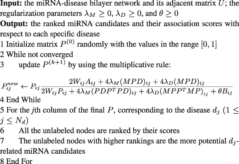
Given an initial value of P, the solution of P can be obtained iteratively by using the above updating rule. The iterative process terminates when the difference between the values of L(P) at the kth iteration and at the (k + 1)th is less than . At last, in terms of disease dj, jth column contains the association scores between dj and all the miRNAs including the labeled nodes and the unlabeled nodes. Since a higher score reveals a more possible association between a miRNA candidate and dj, all the unlabeled nodes are ranked by their scores. The iterative algorithm of predicting disease miRNAs is demonstrated in Figure 3.
Fig. 3.
Iterative algorithm for predicting the miRNA candidates associated with diseases
3 Results and discussion
3.1 Data preparation
The human miRNA-disease database (HMDD) has collected thousands of the miRNA-disease association pairs that had been confirmed by the biological experiments (Li et al., 2014a). As done in previous work (Chen and Chen, 2014; Wang et al., 2010; Xuan et al., 2015), we merged the redundant miRNA-disease associations that produce the same mature miRNAs and obtained 5090 distinct associations between 490 miRNAs and 326 diseases. The disease terms within the disease directed acyclic graphs and their hierarchies were acquired from the U.S. National Library of Medicine (MeSH, http://www.ncbi.nlm.nih.gov/mesh).
3.2 Performance evaluation metrics
To evaluate our approach and the state-of-the-art disease-miRNA-prediction methods, 5-fold cross validation was performed for the well-characterized diseases firstly. For a specific disease d that has known related miRNAs, the d-related miRNAs (labeled nodes) were randomly divided into 5 subsets, 4 of which were used for training a prediction model, while the left out subset was added into a dataset for testing. The testing dataset also contains all the miRNAs that have not been observed to be associated with d (unlabeled nodes). The labeled and unlabeled nodes are regarded as the positive samples and the negative ones, respectively. After the association scores of the testing samples are estimated, the samples will be ranked by their scores. The higher the positive samples are ranked, the better the prediction performance is.
We are also interested in evaluating the ability to correctly identify the miRNAs associated with the new diseases. As there is no any miRNA observed to be related to a new disease so far, the evaluation is simulated by using a disease with known related miRNAs, such as d, and removing all the d-related associations in the training process. In this way, d-related miRNA candidates are predicted by only exploiting the information about the remaining diseases. All the removed d-related miRNAs are taken as positive samples for testing.
Given a threshold δ, if the score of a labeled node is greater than δ, it is deemed as a correctly identified positive sample. If the score of an unlabeled node is smaller than δ, it is a successfully identified negative sample. To obtain a receiver operating characteristic (ROC) curve, the true positive rates (TPRs) and the false positive rates (FPRs) at various δ values are calculated,
| (22) |
where TP and TN are the numbers of correctly identified positive and negative samples. FP and FN are the numbers of misidentified positive and negative samples. The area under the ROC curve (AUC) is used to measure the global performance of a prediction method.
In addition, the top section of prediction result is usually selected by the biologists to further validate with the wet-lab experiments, and the more accurate top k candidates contribute to the success of discovering the novel disease miRNAs. Therefore, the recall rates within top 30, 60, … and 240 candidates are demonstrated, which reveals how many positive samples are successfully recovered within top k. Moreover, the proportion of misidentified negative samples and the proportion of total positive and negative samples identified correctly within top k ranking list are shown as well.
In the current miRNA-disease association data, most of diseases are only associated with several miRNAs, which results in lack of sufficient associations to evaluate the prediction performance. Hence we performed the cross-validation and simulation experiments on 15 well-characterized diseases each of which has at least 80 related miRNAs.
3.3 Comparison with other methods
As most of previous methods can only be applied to the well-characterized diseases, we estimated the prediction performances on these diseases and the new ones, respectively. Firstly, our method, DMPred, was compared with RWRMDA (Chen, 2012), Chen’s method (Chen and Zhang, 2013), RLSMDA (Chen and Chen, 2014), MIDP (Xuan et al., 2015) and Liu’s method (Liu et al., 2016) which are state-of-the-art prediction methods for the well-characterized diseases.
The regularization parameters of each method should be tuned to obtain its best performance. The parameters λM, λD and θ of DMPred were chosen from 1/10, 1/30,…, 1/90, 1, 10, 30,…, 90. The parameter r for both RWRMDA and Chen’s method varied from 0.1 to 0.9. As its literature suggested, the parameters ηM and ηD of RLSMDA were set as 1 according to the prior knowledge, and w ranged from 0.1 to 0.9. The parameters rQ and rU of MIDP and the parameters γ, λ, δ and η of Liu’s method ranged from 0.1 to 0.9. The performances of these methods obtained by using the optimum parameters are demonstrated in Table 1 (λM = 1/70, λD = 1/10 and θ = 1/20 for DMPred, r = 0.9 for RWRMDA, r = 0.8 for Chen’s method, ηM = 1, ηD = 1 and w = 0.9 for RLSMDA, rQ = 0.4 and rU = 0.1 for MIDP, γ = 0.5, λ = 0.8, δ = 0.9 and η = 0.1 for Liu’s method).
Table 1.
Prediction results of DMPred and other methods for the well-characterized diseases
| Disease name | AUC | |||||
|---|---|---|---|---|---|---|
| DMPred | RWRMDA | Chen’s method | RLSMDA | MIDP | Liu’s method | |
| Acute myeloid leukemia | 0.896 | 0.839 | 0.716 | 0.853 | 0.913 | 0.878 |
| Breast neoplasms | 0.940 | 0.785 | 0.653 | 0.832 | 0.838 | 0.847 |
| Colorectal neoplasms | 0.839 | 0.793 | 0.662 | 0.831 | 0.845 | 0.850 |
| Glioblastoma | 0.906 | 0.680 | 0.607 | 0.714 | 0.786 | 0.841 |
| Heart failure | 0.986 | 0.722 | 0.761 | 0.738 | 0.821 | 0.815 |
| Hepatocellular carcinoma | 0.902 | 0.749 | 0.613 | 0.794 | 0.807 | 0.835 |
| Lung neoplasms | 0.945 | 0.827 | 0.606 | 0.855 | 0.876 | 0.912 |
| Melanoma | 0.911 | 0.784 | 0.642 | 0.807 | 0.837 | 0.852 |
| Ovarian neoplasms | 0.928 | 0.882 | 0.644 | 0.909 | 0.923 | 0.898 |
| Pancreatic neoplasms | 0.915 | 0.871 | 0.684 | 0.887 | 0.945 | 0.899 |
| Prostatic neoplasms | 0.950 | 0.823 | 0.629 | 0.841 | 0.882 | 0.857 |
| Renal cell carcinoma | 0.899 | 0.815 | 0.627 | 0.839 | 0.862 | 0.820 |
| Squamous cell carcinoma | 0.901 | 0.819 | 0.676 | 0.849 | 0.870 | 0.877 |
| Stomach neoplasms | 0.901 | 0.779 | 0.628 | 0.797 | 0.821 | 0.827 |
| Urinary bladder neoplasms | 0.924 | 0.821 | 0.632 | 0.845 | 0.897 | 0.863 |
As shown in Table 1, the average AUCs of DMPred, RWRMDA, Chen’s method, RLSMDA, MIDP and Liu’s method on the 15 tested diseases are 91.63, 79.93, 65.20, 82.61, 86.15 and 85.81%, respectively. DMPred performed the best for most of these diseases and its average AUC is 11.7, 26.43, 9.02, 5.48 and 5.82% higher than the other methods, respectively. Note that MIDP and RWRMDA exploited the information of miRNA network, and Chen’s method utilized the information of disease network. DMPred, RLSMDA and Liu’s method not only concentrated on miRNA network but also on disease network, and they all achieved relatively better performances. Chen’s method worked much worse than the other methods, primarily because it did not use the information of miRNA network. Therefore, the use and integration of information of miRNAs and diseases are essential. The improvement of DMPred over the existing methods is mainly due to its seamless integration of multiple kinds of information.
In addition, a paired t-test was performed to measure whether DMPred’s AUCs across 15 diseases are significantly higher than another method. The p-values are listed in Table 2. The statistical result indicates DMPred achieves significantly better performance than all of other methods at the significance level 0.05.
Table 2.
A pairwise comparison with a paired t-test on the prediction results based on AUCs
| RWRMDA | Chen’s method | RLSMDA | MIDP | Liu’s method | |
|---|---|---|---|---|---|
| P-value between DMPred and another method | 2.9441e-06 | 1.8670e-12 | 4.1391e-05 | 8.4149e-04 | 7.3586e-05 |
The higher recall value within top k ranking list means the more positive testing samples (real disease-related miRNAs) are identified successfully. The average recall values across 15 tested diseases within the top k candidates are shown in Figure 4. DMPred consistently outperformed the other methods at various k cutoffs, and ranked 49.6% of positive samples in top 30, 87.1% in top 90 and 97.8% in top 150. MIDP had the second-best accuracy and ranked 43.6% in top 30, 78.4% in top 90 and 90.9% in top 150. Liu’s method ranked 41.8% in top 30, 77.2% in top 90 and 89.0% in top 150, which is worse than MIDP but better than RLSMDA (32.8, 73.4 and 86.9%). RWRMDA achieved inferior performance and its corresponding recall rates are 26.7, 68.4 and 83.7%. Chen’s method ranked 8.5% in top 30, 33.7% in top 90 and 61.3% in top 150, which is still much worse than other methods.
Fig. 4.
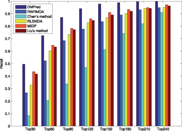
The average recalls across all the tested diseases at different top k values
Specificity measures the proportion of correctly identified negative samples accounting for all the negative samples. Thus, 1-specificity reflects the proportion of misidentified negative samples. A lower 1-specificity value on the top k ranking list means less negative samples are misidentified. As shown in Figure 5, DMPred yields the lowest 1-specificity values at different k cutoffs. In addition, accuracy is the proportion of true positive and negative samples that are identified correctly. DMPred also achieves higher accuracies than the other methods at various k values (Fig. 6).
Fig. 5.
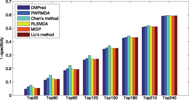
The average 1-specificity values across all the tested diseases at different top k values
Fig. 6.
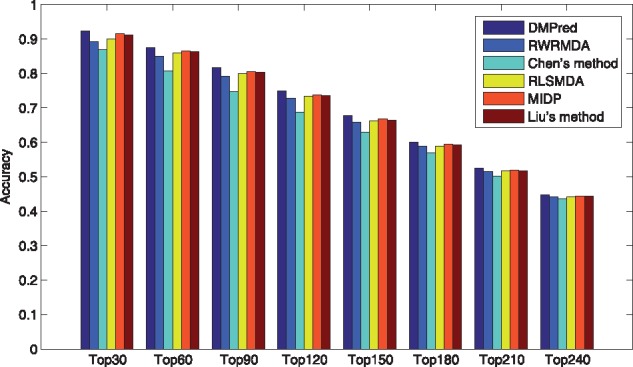
The average accuracies across all the tested diseases at different top k values
To evaluate DMPred’s performance for the new diseases without known related miRNAs, we performed the simulation experiments on the same 15 diseases as the ones in cross validation procedure. Unlike the cross validation experiments, all the associations related to a tested disease d were removed during training period. This operation ensured that predicting d-related candidates only utilized the association information of the remaining diseases and the miRNA and disease similarity information of MiRDisNet. All the removed d-related miRNAs were taken as the positive testing samples.
As only RLSMDA, MIDP and Liu’s method can be applied to the new diseases, DMPred was compared with them and the results are shown in Table 3. The average AUCs of DMPred, RLSMDA, MIDP and Liu’s method across 15 diseases are 0.876, 0.837, 0.839 and 0.832. DMPred consistently performed the best for nearly all of 15 diseases, and MIDP achieved slightly better performance than RLSMDA for most of the diseases. The performance of Liu’s method is relatively inferior. The primary reason is that DMPred considered the correlation between the candidates of various diseases, relative to MIDP and Liu’s method. Meanwhile, DMPred integrated the multiple kinds of information within MiRDisNet completely, relative to RLSMDA. In addition, the p-values of DMPred versus other three methods obtained by performing the paired t-test are 1.7635e-04, 4.4946e-06 and 9.4690e-06. It confirms DMPred’s performance is also significantly higher in terms of the new diseases. In addition, DMPred consistently had the highest average recall rates (Fig. 7), the lowest 1-specificity values (Fig. 8) and the highest accuracies (Fig. 9) on 15 tested diseases at different top k cutoffs.
Table 3.
Prediction results of DMPred and the other methods for the diseases whose respective associations were removed
| Disease name | AUC | |||
|---|---|---|---|---|
| DMPred | RLSMDA | MIDP | Liu’s method | |
| Acute myeloid leukemia | 0.868 | 0.852 | 0.860 | 0.864 |
| Breast neoplasms | 0.877 | 0.803 | 0.821 | 0.806 |
| Colorectal neoplasms | 0.856 | 0.812 | 0.829 | 0.815 |
| Glioblastoma | 0.868 | 0.831 | 0.833 | 0.828 |
| Heart failure | 0.895 | 0.792 | 0.814 | 0.801 |
| Hepatocellular carcinoma | 0.865 | 0.789 | 0.804 | 0.785 |
| Lung neoplasms | 0.921 | 0.897 | 0.874 | 0.878 |
| Melanoma | 0.876 | 0.817 | 0.825 | 0.817 |
| Ovarian neoplasms | 0.906 | 0.894 | 0.876 | 0.875 |
| Pancreatic neoplasms | 0.891 | 0.895 | 0.891 | 0.891 |
| Prostatic neoplasms | 0.854 | 0.844 | 0.829 | 0.827 |
| Renal cell carcinoma | 0.878 | 0.809 | 0.824 | 0.810 |
| Squamous cell carcinoma | 0.886 | 0.883 | 0.864 | 0.865 |
| Stomach neoplasms | 0.844 | 0.781 | 0.806 | 0.788 |
| Urinary bladder neoplasms | 0.860 | 0.852 | 0.836 | 0.832 |
Fig. 7.
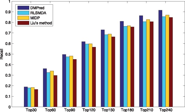
The average recalls across all the simulated new diseases at different top k values
Fig. 8.
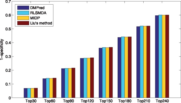
The average 1-specificity values across all the simulated new diseases at different top k values
Fig. 9.
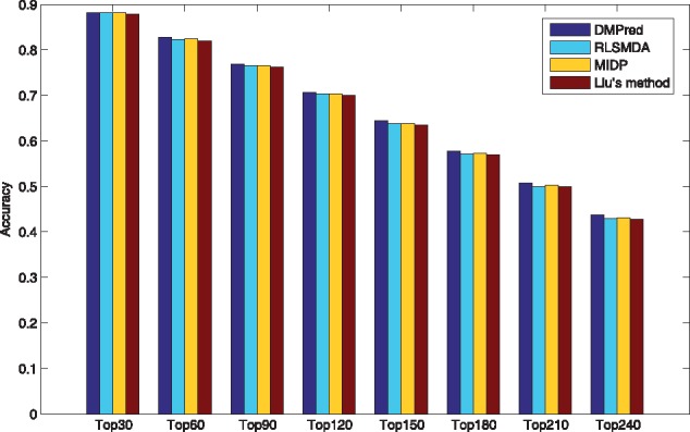
The average accuracies across all the simulated new diseases at different top k values
3.4 Comparison with the prediction instance without sparse penalty
In order to validate the effect of exploiting sparseness characteristic, we further compared the prediction instance with sparse penalty (DMPred) and the one without penalty (DMPred*). The penalty item was eliminated from the original objective function L(P) to form a new function . The prediction instance based on is referred to as DMPred*. As shown in Table 4, the left part demonstrates the results by performing 5-fold cross validation over 15 diseases, and the right part lists the results of simulation experiments after removing the associations related to the tested disease. DMPred achieves consistently higher prediction performances than DMPred* for the well-characterized diseases and the simulated new ones. In terms of the well-characterized diseases, AUC of DMPred increased at least by 1.1%, increased at most by 9.7% and increased by 5.2% on average. For the new diseases, AUC of DMPred increased at least by 1.4%, increased at most by 5.5% and increased by 4% on average. It indicates that introducing sparse penalty is effective for the improvement of the discriminative ability of prediction model.
Table 4.
Prediction results obtained by performing the prediction instance with sparse penalty (DMPred) and the one without sparse penalty (DMPred*)
| Disease name | AUC | |||
|---|---|---|---|---|
| DMPred | DMPred* | DMPred | DMPred* | |
| Acute myeloid leukemia | 0.896 | 0.835 | 0.868 | 0.821 |
| Breast neoplasms | 0.940 | 0.874 | 0.877 | 0.850 |
| Colorectal neoplasms | 0.839 | 0.813 | 0.856 | 0.804 |
| Glioblastoma | 0.906 | 0.822 | 0.868 | 0.840 |
| Heart failure | 0.986 | 0.929 | 0.895 | 0.877 |
| Hepatocellular carcinoma | 0.902 | 0.805 | 0.865 | 0.842 |
| Lung neoplasms | 0.945 | 0.913 | 0.921 | 0.876 |
| Melanoma | 0.911 | 0.824 | 0.876 | 0.862 |
| Ovarian neoplasms | 0.928 | 0.910 | 0.906 | 0.851 |
| Pancreatic neoplasms | 0.915 | 0.904 | 0.891 | 0.808 |
| Prostatic neoplasms | 0.950 | 0.891 | 0.854 | 0.814 |
| Renal cell carcinoma | 0.899 | 0.855 | 0.878 | 0.858 |
| Squamous cell carcinoma | 0.901 | 0.824 | 0.886 | 0.837 |
| Stomach neoplasms | 0.901 | 0.830 | 0.844 | 0.801 |
| Urinary bladder neoplasms | 0.924 | 0.872 | 0.860 | 0.807 |
3.5 Case studies: breast neoplasms, colorectal neoplasms, lung neoplasms and 32 diseases
To further demonstrate DMPred’s ability to discover potential disease miRNA candidates for the well-characterized diseases, we executed the case studies on breast neoplasms, colorectal neoplasms and lung neoplasms. The top 50 candidates related to breast neoplasms are taken as examples and analyzed in detail.
First, a database named PhenomiR was established to demonstrate the miRNAs which have different expression in disease tissues relative to the normal ones (Ruepp et al., 2010). PhenomiR contained 675 miRNAs that had been identified by analyzing the results of microarray experiments, northern blot experiments and PCR experiments. Similarly, the dbDEMC database included 607 miRNAs that had abnormal expression in 14 kinds of cancers through analysis of microarray datasets (Yang et al., 2010). As shown in Table 5, 39 of 50 candidates are contained by PhenomiR and 39 candidates are included by dbDEMC, which indicates they have been upregulated or downregulated in breast cancer (malignant breast neoplasm).
Table 5.
The top 50 breast neoplasms-related candidates
| Rank | MiRNA name | Description | Rank | MiRNA name | Description |
|---|---|---|---|---|---|
| 1 | hsa-mir-130a | PhenomiR, dbDEMC, miRCancer | 26 | hsa-mir-211 | PhenomiR, dbDEMC, literature1 |
| 2 | hsa-mir-99a | PhenomiR, dbDEMC, miRCancer | 27 | hsa-mir-212 | PhenomiR, dbDEMC |
| 3 | hsa-mir-138 | PhenomiR, dbDEMC, literature1 | 28 | hsa-mir-449b | literature2 |
| 4 | hsa-mir-192 | PhenomiR, dbDEMC | 29 | hsa-mir-181c | PhenomiR, dbDEMC |
| 5 | hsa-mir-142 | PhenomiR, literature1 | 30 | hsa-mir-144 | PhenomiR, dbDEMC |
| 6 | hsa-mir-378a | PhenomiR, dbDEMC | 31 | hsa-mir-302f | literature1 |
| 7 | hsa-mir-106a | PhenomiR, dbDEMC | 32 | hsa-mir-574 | dbDEMC |
| 8 | hsa-mir-130b | PhenomiR, dbDEMC | 33 | hsa-mir-491 | PhenomiR, dbDEMC |
| 9 | hsa-mir-15b | PhenomiR, dbDEMC | 34 | hsa-mir-184 | PhenomiR, dbDEMC |
| 10 | hsa-mir-186 | PhenomiR, dbDEMC | 35 | hsa-mir-208a | PhenomiR, dbDEMC |
| 11 | hsa-mir-542 | literature1 | 36 | hsa-mir-371a | PhenomiR |
| 12 | hsa-mir-150 | PhenomiR, dbDEMC, miRCancer | 37 | hsa-mir-363 | dbDEMC |
| 13 | hsa-mir-92b | literature1 | 38 | hsa-mir-190a | literature1 |
| 14 | hsa-mir-95 | PhenomiR, dbDEMC | 39 | hsa-mir-376a | PhenomiR, dbDEMC |
| 15 | hsa-mir-330 | PhenomiR, dbDEMC | 40 | hsa-mir-517a | PhenomiR, dbDEMC |
| 16 | hsa-mir-185 | PhenomiR, dbDEMC | 41 | hsa-mir-503 | dbDEMC |
| 17 | hsa-mir-99b | PhenomiR, dbDEMC, miRCancer | 42 | hsa-mir-302e | literature2 |
| 18 | hsa-mir-449a | PhenomiR, dbDEMC | 43 | hsa-mir-483 | PhenomiR, dbDEMC |
| 19 | hsa-mir-98 | PhenomiR, dbDEMC, miR2disease, miRCancer | 44 | hsa-mir-455 | PhenomiR |
| 20 | hsa-mir-32 | PhenomiR, dbDEMC | 45 | hsa-mir-650 | dbDEMC |
| 21 | hsa-mir-370 | PhenomiR, dbDEMC | 46 | hsa-mir-381 | PhenomiR, dbDEMC |
| 22 | hsa-mir-181d | PhenomiR, dbDEMC, miR2disease | 47 | hsa-mir-30e | PhenomiR |
| 23 | hsa-mir-494 | PhenomiR, dbDEMC, miRCancer | 48 | hsa-mir-744 | dbDEMC |
| 24 | hsa-mir-196b | PhenomiR, dbDEMC, miRCancer | 49 | hsa-mir-134 | PhenomiR, dbDEMC |
| 25 | hsa-mir-372 | PhenomiR, dbDEMC | 50 | hsa-mir-518b | PhenomiR |
Note: (1) ‘PhenomiR’ means that a miRNA was identified to have abnormal expression in breast cancer by analyzing the results of microarray experiments, northern blot experiments and PCR experiments. (2) With analysis of the microarray datasets, a miRNA is considered to have different expression levels in breast cancer compared with normal tissues. This kind of miRNAs is labeled with ‘dbDEMC’. (3) ‘miR2Disease’ means that a miRNA is contained by the manually curated miRNA-disease association database, miR2Disease and confirmed to be associated with breast cancer. (4) ‘miRCancer’ means an association between a miRNA and breast cancer is included by the database miRCancer. (5) ‘literature1’ means that there is a published literature to support that a miRNA is upregulated or downregulated in breast neoplasm, compared with normal breast tissues. (6) ‘literature2’ means that a miRNA is related to some important factors affecting the development of breast neoplasms.
Second, a miRNA-cancer association database, miRCancer, included the experimentally validated 878 associations between 236 miRNAs and 79 cancers (Xie et al., 2013). The associations were extracted from the published literatures by using text mining technique and then the dysregulation cases of the miRNAs were confirmed manually. miR2disease is also a database which contained manually curated miRNAs that had dysregulation in various diseases (Jiang et al., 2009). Seven candidates are contained by miRCancer and 2 candidates are recorded by miR2disease. Therefore, they have been verified to be breast cancer-related miRNAs.
Finally, 9 candidates labeled with ‘literature’ are supported by the published literatures and the detailed interpretation is listed in Supplementary Table ST1. Several studies verified that 7 of 9 miRNAs were dysregulated in breast tumors versus normal breast tissues. In addition, hsa-mir-449b is a direct transcriptional target of E2F1 which is an important transcription factor relative to breast cancer (Yang et al., 2009). Estrogen receptor-alpha (ER-α) has become one of the most important target in breast cancer therapeutics. Hsa-mir-302e was inferred to inhibit the expression levels of ER-α and negatively regulate ER-α-mediated signaling pathways in breast cancer (Li et al., 2014b). Hence hsa-mir-449b and hsa-mir-302e are the promising breast cancer-related candidates.
In terms of colorectal neoplasms, the top 50 candidates are demonstrated in Supplementary Table ST2. Seven candidates were contained by PhenomiR and 40 candidates were included by dbDEMC to have abnormal expression in colorectal cancer. MiR2Disease and miRCancer respectively confirmed that the expression levels of 3 candidates and 13 candidates varied significantly between the colorectal tumors and normal colorectal tissues. Five candidates were supported by the literatures to be dysregulated in colorectal neoplasms.
The top 50 lung neoplasms-related candidates are listed in Supplementary Table ST3. PhenomiR and dbDEMC respectively identified 38 candidates and 43 candidates whose abnormal expressions have been found in lung cancer. miRCancer confirmed 25 candidates to have differential expression in lung tumors versus normal lung tissues. Ten candidates were verified by miR2disease to have been associated with the disease. A candidate was supported by the literature to be dysregulated in lung neoplasms.
In addition, since RLSMDA and MIDP concentrated on 32 new diseases to show their ability to effectively determine the potential candidates, DMPred was also applied to the diseases. The top 3 potential candidates for each disease were validated by the literatures and the related database. Forty-six miRNA-disease associations were supported by the literatures and one association has been recorded by miR2Disease (see details in Supplementary Table ST4). On the whole, the case studies indicate that DMPred has powerful ability to discover potential candidates for not only well-characterized diseases but also new ones.
3.6 Predicting novel disease-related miRNAs
After having confirmed its prediction performance by cross validation and simulation experiments, as well as case studies, we further applied DMPred to all the diseases including the ones with known related miRNAs and the new ones. All the known miRNA-disease associations were taken as training data to predict the novel disease-related miRNAs. The potential candidates for all the diseases are listed in Supplementary Table ST5.
4 Conclusions
A novel method based on non-negative matrix factorization with sparseness constraints, DMPred, was developed for predicting disease miRNAs. DMPred integrated multiple kinds of information within the miRNA-disease bilayer network seamless, which exploited the consensus relationship between them completely. Furthermore, DMPred took the correlation between the candidates of various diseases into account and predicted their respective candidates for all the diseases at the same time. In addition, incorporating the sparseness characteristic of miRNA-disease associations also contributed to the improvement of prediction performance. The results of cross validation and simulation experiments on 15 common diseases confirmed the superiority of DMPred for the well-characterized diseases and the new ones. The case studies on 3 well-characterized diseases and 32 new diseases further demonstrated DMPred’s ability to discover the potential candidates. DMPred will be useful in screening the promising candidates for subsequent studies concerning their involvement in the etiology and pathogenesis of diseases.
Funding
The work was supported by the Natural Science Foundation of China (61302139, 61702296), the United States National Institutes of Health (R01GM100364), the Natural Science Foundation of Heilongjiang Province (F2015013, F201430), the Young Reserve Talents Research Foundation of Harbin Science and Technology Bureau (2015RAQXJ004, 2016RQQXJ135), the China Postdoctoral Science Foundation (2014M550200, 2015T80367), the Postdoctoral Foundation of Heilongjiang Province (LBH-Z14152), and the Distinguished Youth Foundation of Heilongjiang University (JCL201405, QL200702).
Conflict of Interest: none declared.
Supplementary Material
References
- Bandyopadhyay S. (2010) Development of the human cancer microRNA network. Silence, 1, 6.. [DOI] [PMC free article] [PubMed] [Google Scholar]
- Bartel D.P. (2004) MicroRNAs: genomics, biogenesis, mechanism, and function. Cell, 116, 281–297. [DOI] [PubMed] [Google Scholar]
- Bartel D.P. (2009) MicroRNAs: target recognition and regulatory functions. Cell, 136, 215–233. [DOI] [PMC free article] [PubMed] [Google Scholar]
- Calin G.A., Croce C.M. (2006) MicroRNA-cancer connection: the beginning of a new tale. Cancer Res., 66, 7390–7394. [DOI] [PubMed] [Google Scholar]
- Chatterjee S., Grosshans H. (2009) Active turnover modulates mature microRNA activity in Caenorhabditis elegans. Nature, 461, 546–549. [DOI] [PubMed] [Google Scholar]
- Chen H., Zhang Z. (2013) Prediction of associations between OMIM diseases and microRNAs by random walk on OMIM disease similarity network. Sci. World J., 2013, 204658.. [DOI] [PMC free article] [PubMed] [Google Scholar]
- Chen X. (2012) RWRMDA: predicting novel human microRNA-disease associations. Mol. BioSystems, 8, 2792–2798. [DOI] [PubMed] [Google Scholar]
- Chen X., Yan G.Y. (2014) Semi-supervised learning for potential human microRNA-disease association inference. Scientific Reports, 4, 5501. [DOI] [PMC free article] [PubMed] [Google Scholar]
- Goh K.I. et al. (2007) The human disease network. Proc. Natl. Acad. Sci. USA, 104, 8685–8690. [DOI] [PMC free article] [PubMed] [Google Scholar]
- Hamosh A. et al. (2005) Online Mendelian Inheritance in Man (OMIM), a knowledgebase of human genes and genetic disorders. Nucleic Acids Res., 33, D514–D517. [DOI] [PMC free article] [PubMed] [Google Scholar]
- He L., Hannon G.J. (2004) MicroRNAs: small RNAs with a big role in gene regulation. Nat. Rev. Genet., 5, 522–531. [DOI] [PubMed] [Google Scholar]
- Hoehndorf R. et al. (2015) Analysis of the human diseasome using phenotype similarity between common, genetic, and infectious diseases. Sci. Rep., 5, 10888.. [DOI] [PMC free article] [PubMed] [Google Scholar]
- Jiang Q. et al. (2009) miR2Disease: a manually curated database for microRNA deregulation in human disease. Nucleic Acids Res., 37, D98–D104. [DOI] [PMC free article] [PubMed] [Google Scholar]
- Jiang Q. et al. (2010) Prioritization of disease microRNAs through a human phenome-microRNAome network. BMC Syst. Biol., 4, S2. [DOI] [PMC free article] [PubMed] [Google Scholar]
- Kertesz M. et al. (2007) The role of site accessibility in microRNA target recognition. Nat. Genet., 39, 1278–1284. [DOI] [PubMed] [Google Scholar]
- Kosik K.S. (2006) The neuronal microRNA system. Nat. Rev. Neurosci., 7, 911–920. [DOI] [PubMed] [Google Scholar]
- Lewis B.P. et al. (2003) Prediction of mammalian microRNA targets. Cell, 115, 787–798. [DOI] [PubMed] [Google Scholar]
- Li X. et al. (2011) Prioritizing human cancer microRNAs based on genes functional consistency between microRNA and cancer. Nucleic Acids Res., 39, 1–10. [DOI] [PMC free article] [PubMed] [Google Scholar]
- Li Y. et al. (2014a) HMDD v2.0: a database for experimentally supported human microRNA and disease associations. Nucleic Acids Res., 42, D1070–D1074. [DOI] [PMC free article] [PubMed] [Google Scholar]
- Li X. et al. (2014b) A systematic in silico mining of the mechanistic implications and therapeutic potentials of estrogen receptor (ER)-α in breast cancer. PloS ONE, 9, e91894. [DOI] [PMC free article] [PubMed] [Google Scholar]
- Liu B. et al. (2014) Identifying miRNAs, targets and functions. Brief. Bioinf., 15, 1–19. [DOI] [PMC free article] [PubMed] [Google Scholar]
- Liu Y. et al. (2016) Inferring microRNA-disease associations by random walk on a heterogeneous network with multiple data sources. IEEE/ACM Trans. Comput. Biol. Bioinf., 99, 1–11. [DOI] [PubMed] [Google Scholar]
- Lu M. et al. (2008) An analysis of human microRNA and disease associations. PLoS ONE, 3, e3420.. [DOI] [PMC free article] [PubMed] [Google Scholar]
- Meola N. et al. (2009) MicroRNAs and genetic diseases. Pathogenetics, 2, 1. [DOI] [PMC free article] [PubMed] [Google Scholar]
- Natarajan N., Dhillon I.S. (2014) Inductive matrix completion for predicting gene Cdisease associations. Bioinformatics, 30, i60–i68. [DOI] [PMC free article] [PubMed] [Google Scholar]
- Ritchie W. et al. (2009) Predicting microRNA targets and functions: traps for the unwary. Nat. Methods, 6, 397–398. [DOI] [PubMed] [Google Scholar]
- Ruepp A. et al. (2010) PhenomiR: a knowledgebase for microRNA expression in diseases and biological processes. Genome Biol., 11, R6.. [DOI] [PMC free article] [PubMed] [Google Scholar]
- Sayed D., Abdellatif M. (2011) MicroRNAs in development and disease. Physiol. Rev., 91, 827–887. [DOI] [PubMed] [Google Scholar]
- Shi H. et al. (2013) Walking the interactome to identify human miRNA-disease associations through the functional link between miRNA targets and disease genes. BMC Syst. Biol., 7, 101. [DOI] [PMC free article] [PubMed] [Google Scholar]
- Tan V.Y., Févotte C. (2009) Automatic relevance determination in nonnegative matrix factorization. In: SPARS’09-Signal Processing with Adaptive Sparse Structured Representations.
- Wang D. et al. (2010) Inferring the human microRNA functional similarity and functional network based on microRNA-associated diseases. Bioinformatics, 26, 1644–1650. [DOI] [PubMed] [Google Scholar]
- Weinreich S.S. et al. (2008) Orphanet: a European database for rare diseases. Nederlands Tijdschrift Voor Geneeskunde, 152, 518–519. [PubMed] [Google Scholar]
- Xie B. et al. (2013) miRCancer: a microRNA Ccancer association database constructed by text mining on literature. Bioinformatics, 29, 638–644. [DOI] [PubMed] [Google Scholar]
- Xuan P. et al. (2013) Prediction of microRNAs associated with human diseases based on weighted k most similar neighbors. PLoS ONE, 8, e70204. [DOI] [PMC free article] [PubMed] [Google Scholar]
- Xuan P. et al. (2015) Prediction of potential disease-associated microRNAs based on random walk. Bioinformatics, 31, 1805–1815. [DOI] [PubMed] [Google Scholar]
- Yang X. et al. (2009) MiR-449a and miR-449b are direct transcriptional targets of E2F1 and negatively regulate pRb-E2F1 activity through a feedback loop by targeting CDK6 and CDC25A. Genes Dev., 23, 2388–2393. [DOI] [PMC free article] [PubMed] [Google Scholar]
- Yang Z. et al. (2010) dbDEMC: a database of differentially expressed miRNAs in human cancers. BMC Genomics, 11, S5. [DOI] [PMC free article] [PubMed] [Google Scholar]
Associated Data
This section collects any data citations, data availability statements, or supplementary materials included in this article.


