

Abstract
Decision-making requires choosing from treatments on the basis of correctly estimated outcome distributions under each treatment. In the absence of randomized trials, 2 possible approaches are the parametric g-formula and agent-based models (ABMs). The g-formula has been used exclusively to estimate effects in the population from which data were collected, whereas ABMs are commonly used to estimate effects in multiple populations, necessitating stronger assumptions. Here, we describe potential biases that arise when ABM assumptions do not hold. To do so, we estimated 12-month mortality risk in simulated populations differing in prevalence of an unknown common cause of mortality and a time-varying confounder. The ABM and g-formula correctly estimated mortality and causal effects when all inputs were from the target population. However, whenever any inputs came from another population, the ABM gave biased estimates of mortality—and often of causal effects even when the true effect was null. In the absence of unmeasured confounding and model misspecification, both methods produce valid causal inferences for a given population when all inputs are from that population. However, ABMs may result in bias when extrapolated to populations that differ on the distribution of unmeasured outcome determinants, even when the causal network linking variables is identical.
Keywords: agent-based models, causal inference, decision analysis, individual-level models, mathematical models, medical decision making, Monte Carlo methods, parametric g-formula
Editor's note: Invited commentaries on this article appear on pages 143 and 000.
Clinical and public health decision-making requires choices among treatment strategies. For these decisions to be sound, researchers need to correctly estimate the distribution of the outcome—survival, cost-effectiveness, or another utility function—under each of the candidate strategies. When a randomized trial of these strategies is not feasible, agent-based models (ABMs) (1, 2) and the parametric g-formula (3, 4) are 2 alternative analytical approaches. We compared the relative advantages and disadvantages of these 2 approaches.
The parametric g-formula has been exclusively applied to data from a single prospective study. This reflects the fact that parameter estimates of both the model parameters and intervention distributions based on the data from one population cannot be extrapolated to a second population, except under strong assumptions. As a result, inferences from the parametric g-formula are restricted to populations similar to the study population and to the time horizon and treatment strategies that are observed in the data. In contrast, ABMs combine data from multiple sources, so they are viewed as tools to make more generalized inferences that are not constrained by the population characteristics, time horizon, and treatment strategies observed in any particular study (5).
The greater flexibility of ABMs makes them a key tool for clinical and public health decision-making. However, this greater flexibility comes at a price: For the extrapolations to be correct, the model needs to make implicit or explicit assumptions about the distribution of unmeasured determinants of the outcome that do not confound the effect of interest, given the measured variables. In contrast, because it is not used for extrapolation, the parametric g-formula can be agnostic about the distribution of unmeasured nonconfounders. As a consequence, the input parameters of ABMs are often implicitly (and frequently incorrectly) endowed with a causal interpretation, whereas the input parameters of the parametric g-formula do not necessarily receive a causal interpretation. In other words, the components of ABMs are specified as causal models to yield causal estimates in many populations, whereas the parametric g-formula uses noncausal models to yield causal estimates in a single population (3, 4).
Despite these different interpretations, ABMs and the parametric g-formula use a similar mathematical approach: construction of a sequential model that is the basis for a Monte Carlo simulation of a (counterfactual) population under each treatment strategy of interest. However, ABMs and the parametric g-formula have generally been considered in isolation, and there is typically little overlap in the population of researchers familiar with each method (6, 7).
In this paper we explore the practical consequences of the different interpretation of the model parameters between ABMs and the parametric g-formula. We start with the description of a simplified decision analysis example; the goal is to determine whether we can decrease the 12-month mortality risk of HIV-positive individuals by offering them antiretroviral therapy.
A SIMPLIFIED DECISION-ANALYSIS EXAMPLE
Let Ak be an indicator for initiation of antiretroviral treatment in month k, Lk an indicator for high CD4 cell count (defined as ≥350 cells/μL) measured at the beginning of month k, and Yk+1 an indicator for death by the beginning of month k + 1. We use overbars to represent history. For example, an individual with a high CD4 cell count in months 0 and 1, and low in month 2, has CD4 count history .
As shown in the decision tree (1, 8) depicted in Figure 1, a decision to start treatment may be more likely when previous CD4 cell counts are low, which indicates a worse prognosis (9). Therefore an individual's probability of initiating treatment at k, , depends on her CD4 cell count history. To simplify, we assume that treatment, once initiated, is maintained until death. The probabilities of having a low CD4 cell count, , and of dying, , for an individual alive in month k depend on her CD4 cell count and treatment history.
Figure 1.
Simplified decision process for the use of treatment among HIV-positive individuals at each month k. Square black nodes represent decision points where intervention is possible, white circles represent nodes where an individual's path depends on the conditional probability distribution specified, and triangles represent terminal nodes.
Suppose we are interested in the effect of treatment on 12-month mortality risk. We might specify treatment strategies, such as “always treat” and “never treat.” We can then create an ABM where treatment at each time point is assigned based on one of these strategies and compare the (counterfactual) 12-month mortality risk under each. Similarly, we can use the parametric g-formula to estimate these mortality risks.
Agent-based model
The model is defined by nonoverlapping, mutually exclusive states based on Lk (i.e., low and high CD4 cell count) and Yk (i.e., dead and alive) specified by the investigators. The transition probabilities and govern movement between states conditional on prior history. These probabilities are obtained from published sources, including randomized trials and observational studies (10). The dependence of these probabilities on prior history is often achieved through modeling. For example, a model for the monthly conditional probability of mortality may be , where h(t) is a flexible function (e.g., restricted cubic splines) of time k, and the vector of parameters β is replaced by published estimates from a similar model fitted to data from a particular population. Similarly, a model for the monthly conditional probability of high CD4 cell count may be where the vector of estimated parameters is also obtained from one or more observational studies or randomized trials that may differ from the study used to estimate the model for Yk.
Investigators then use these models to simulate individuals’ trajectories under a strategy of interest. For example, if we were interested in comparing the 12-month mortality risk under the strategies “always treat” and “never treat,” we would set the probability of treatment to 1 for all times and conduct a Monte Carlo simulation (1) with a large number of simulated individuals and, separately, set the probability of treatment to 0 at all times and conduct another Monte Carlo simulation. The 12-month mortality risks estimated from these simulations would then be compared.
The parametric g-formula
The implementation of the parametric g-formula (3, 4, 11) has the same 2 steps as that of ABMs: specification of parametric models for and followed by Monte Carlo simulation under the treatment strategies of interest. The parameters of these models are estimated from a single study (here, a follow-up study of HIV-positive individuals with monthly measurements of CD4 cell count, treatment, and mortality). The parametric g-formula could be based on exactly the same parametric models that define the ABM. Then the mortality under different treatment strategies is estimated by simulation as described above.
ABM users routinely make inferences across settings, populations, and time frames. This extrapolation generally requires that the model parameters are interpreted as causal effects. In contrast, this causal interpretation has not been necessary for the parametric g-formula because users have exclusively restricted their inferences to settings, populations, and time frames very similar to those of the study population. In the next section we examine the implications of this different interpretation of the model parameters when treatment-confounder feedback exists.
TREATMENT-CONFOUNDER FEEDBACK
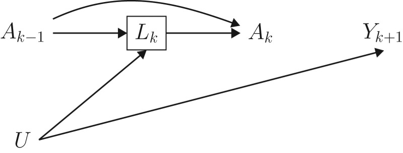
The causal diagram in Figure 2 represents 2 time points for the setting described in the previous sections. We say that there is treatment-confounder feedback because, at each time point k, the confounder CD4 cell count Lk affects subsequent treatment Ak and is affected by prior treatment Ak−1. The causal diagram also includes an unmeasured prognostic factor U which independently affects both the confounder CD4 cell count and the mortality outcome. Unmeasured common causes of confounders and outcome are likely to exist in most settings. In our example U could represent the underlying damage to the immune system.
Figure 2.
Causal directed acyclic graph depicting 2 arbitrary time points from a setting with a time-varying treatment A that has no causal effect on the outcome Y. Conventional adjustment for the confounder L by regression or stratification is expected to introduce bias, because L is affected by prior treatment and shares a cause (U) with the outcome.
The simultaneous presence of treatment-confounder feedback and the unmeasured U prevents conventional methods (e.g., outcome regression) that adjust for the confounder Lk from validly estimating the counterfactual probabilities or causal effects (even when null) under the treatment strategies of interest. The variable Lk is referred to as a collider on the path from Ak−1 to Yk because it is a common effect of 2 variables (Ak−1 and U) on that path. Because conditioning on a collider will generally induce an association between its causes (12), conditioning on Lk would create an association between Ak−1 and U, and therefore between Ak−1 and Yk (because U is associated with Yk).
As an example, consider the outcome regression model for described in the previous section. The parameter β5 for past treatment quantifies the conditional association between Ak−1 and Yk. Part of this association may be due to the direct causal effect on Ak−1 on Yk that is not mediated through Lk and the other variables in the model, and another part of this association may be due to bias because of conditioning on Lk. That is, the parameter β5 is expected to be nonzero even if treatment Ak−1 had no effect on any individual's outcome Yk and therefore cannot be interpreted causally as the direct effect of past treatment that is not mediated through the other variables in the model.
The impossibility of endowing the parameter β5 with a causal interpretation is not a problem for the parametric g-formula, which simply uses the models for and as an intermediate step to estimate the counterfactual probability of death in the study population (3, 4). ABMs, on the other hand, implicitly endow individual model parameters with a causal interpretation to allow for extrapolation to new populations. Thus the parameter β5 in the outcome model of the ABM is interpreted as the direct effect of Ak−1 on Yk. This can result in biased estimates of counterfactual risks and causal effects (even when null). In fact, as we discuss in Appendix 1, such biases may even occur when U is a cause of Lk or Yk but not both, if the effect of treatment is non-null.
In the next section, we present simulation studies that quantify this bias in our example with multiple treatment decisions over time when ABMs are used to extrapolate from one population to another. Because the bias in extrapolating risk from one population to the other is affected by the mortality risks in the absence of treatment, our simulations include scenarios with different underlying mortality risks. The results for both risks and causal contrasts follow directly from the g-formula (see Appendix 1, Appendix Figures 1–4, and Appendix Tables 1–4) and, for risks, also from the graphical results of Bareinboim and Pearl (13, 14). In all simulations an unmeasured variable U was a common cause of the Lk and Yk. Appendix 1 considers the case when this is not so.
SIMULATIONS UNDER A NULL TREATMENT EFFECT
We simulated 3 scenarios by varying the distribution of the unmeasured variable U in Figure 2: a base scenario with a 12-month risk of approximately 10%, a high-risk scenario with a risk of approximately 50%, and a low-risk scenario with a risk of approximately 1%. For each scenario, we simulated a cohort of 105 HIV-positive individuals followed for 12 months under the data-generating mechanism in Figure 2. We simulated monthly CD4 count, treatment, and death status, with no missing data, for each individual. Treatment had no effect on mortality, which could represent the comparison of 2 active treatments of equal effectiveness or the comparison of an ineffective treatment with no treatment. (To simplify the simulations, we let U correspond to a subject's time of death under no treatment.)
In each scenario, we estimated the counterfactual 12-month mortality risk under the treatment strategies “always treat” and “never treat.” We first estimated these risks using the parametric g-formula applied to the simulated data. We then estimated these risks using ABMs with the same model specification as the parametric g-formula.
In the high- and low-risk scenarios, we implemented 4 ABMs depending on the origin of the model parameters:
The scenario of interest (high or low risk). ABM 1 is expected to provide an unbiased risk estimate and thus an unbiased estimate of the null causal effect of treatment.
The base scenario. ABM 2 is expected to provide a risk estimate that is unbiased for the base scenario but biased for the high- and low-risk scenarios, because of nontransportability. However, the estimate of the causal effect should correctly be null.
The parameter for prior treatment β5 from the base scenario and all other parameters from the scenario of interest. ABM 3 is expected to provide biased risk estimates. In fact, the estimate of the null causal effect is expected to be biased, because the magnitude of the association between prior treatment and the outcome conditional on a collider generally varies across populations with different outcome risk in the absence of treatment.
The parameter for prior treatment β5 from the scenario of interest and all other parameters from the base scenario. Like ABM 3, ABM 4 is expected to provide biased estimates of risks and the null causal effect.
The data were simulated following the algorithm described by Robins (15) and Young et al. (16) (Web Appendix 1 and Web Table 1, available at https://academic.oup.com/aje). We estimated the 12-month risk of death and effect of treatment on the additive scale using the g-formula and each of the 4 ABMs in each population (Web Appendix 2 and Web Table 2). SAS, version 9.4 (SAS Institute, Inc., Cary, North Carolina), was used for all analyses, and the code is provided in Web Appendix 3.
SIMULATION RESULTS
The first row of Table 1 shows the 12-month mortality risk in the 3 simulated scenarios.
Table 1.
Null Treatment Effect Simulation: 12-Month Risk of Death Estimated Under 2 Interventions in Different Scenarios
| Estimation Method and Intervention | Base Scenario | High-Risk Scenario | Low-Risk Scenario | |||
|---|---|---|---|---|---|---|
| 12-Month Risk, % | 95% CI | 12-Month Risk, % | 95% CI | 12-Month Risk, % | 95% CI | |
| Simulated data | 10.8 | 47.9 | 1.2 | |||
| Parametric g-formula | ||||||
| Always treat | 10.6 | 10.3, 10.9 | 47.6 | 47.3, 47.9 | 1.1 | 1.0, 1.2 |
| Never treat | 10.5 | 10.2, 10.8 | 47.7 | 47.4, 48.0 | 1.2 | 1.1, 1.3 |
| Risk difference | 0.1 | −0.4, 0.5 | −0.1 | −0.5, 0.4 | −0.1 | −0.3, 0.1 |
| ABM 1a | ||||||
| Always treat | 10.6 | 47.6 | 1.1 | |||
| Never treat | 10.5 | 47.7 | 1.2 | |||
| Risk difference | 0.1 | −0.1 | −0.1 | |||
| ABM 2b | ||||||
| Always treat | 10.6 | 10.6 | ||||
| Never treat | 10.5 | 10.5 | ||||
| Risk difference | 0.1 | 0.1 | ||||
| ABM 3c | ||||||
| Always treat | 22.3 | 2.1 | ||||
| Never treat | 47.7 | 1.2 | ||||
| Risk difference | −25.4 | 1.0 | ||||
| ABM 4d | ||||||
| Always treat | 29.9 | 5.7 | ||||
| Never treat | 10.5 | 10.5 | ||||
| Risk difference | 19.4 | −4.8 | ||||
Abbreviations: ABM, agent-based model; CI, confidence interval.
a All parameters from scenario of interest.
b All parameters from base scenario.
c Parameter for past treatment from base scenario; all others from scenario of interest.
d Parameter for past treatment from scenario of interest; all others from base scenario.
Table 1 shows estimates under “always treat” and “never treat” for the parametric g-formula and ABM 1. As expected under the null, both methods estimated identical risks. Table 1 shows the 95% confidence intervals around the g-formula estimates. (Owing to the so-called “null paradox” (17), one might be concerned that the parametric models used in the g-formula are misspecified and bias might result. However, in the simulation studies performed here, this bias will be much less than the standard error, so the “null paradox” can be safely ignored throughout.) See Web Appendix 4 and Web Table 3 for uncertainty intervals around the ABM estimates (18). Although the uncertainty intervals obtained from these sensitivity analyses are not interpretable as confidence intervals, they can provide some insight into the range of possible outcome distributions consistent with variations of the model (19).
Next, Table 1 shows estimates for ABMs 2, 3, and 4 for the high- and low-risk scenarios. ABM 2 predictably replicates the g-formula estimates from the base scenario, and the risk estimates are therefore biased for the high- and low-risk scenarios. However, because the effect is null in all populations, the causal effect estimate from ABM 2 is correct for the high- and low-risk scenarios. ABM 3 and ABM 4 yield biased estimates of the risk and causal effect for both scenarios.
SIMULATIONS UNDER A NON-NULL TREATMENT EFFECT
We conducted 2 additional sets of simulations that were identical to the one described above except that the treatment effects were non-null. In one, treatment was designed to have a harmful effect on survival, with treated individuals expected to have a mortality rate approximately twice that of as untreated individuals. In the second, treatment was designed to have a beneficial effect on survival, such that individuals who were treated were expected to have a mortality rate approximately half that of individuals who were untreated.
When the treatment was harmful, 12-month risk increased in all scenarios (Table 2). As expected, ABM 2 replicated the base scenario 12-month mortality. However, since the treatment effect was no longer null, the causal effect estimates from ABM 2 were now biased for the high- and low-risk populations. ABMs 3 and 4 remained biased for both the high- and low-risk scenarios.
Table 2.
Harmful Treatment Effect Simulation: 12-Month Risk of Death Estimated Under 2 Interventions in Different Scenarios
| Estimation Method and Intervention | Base Scenario | High-Risk Scenario | Low-Risk Scenario | |||
|---|---|---|---|---|---|---|
| 12-Month Risk, % | 95% CI | 12-Month Risk, % | 95% CI | 12-Month Risk, % | 95% CI | |
| Simulated data | 18.3 | 56.1 | 2.2 | |||
| Parametric g-formula | ||||||
| Always treat | 23.1 | 23.0, 23.2 | 64.3 | 64.2, 64.4 | 2.8 | 2.7, 2.8 |
| Never treat | 10.7 | 10.6, 10.8 | 46.2 | 46.1, 46.3 | 1.2 | 1.2, 1.2 |
| Risk difference | 12.4 | 12.3, 12.6 | 18.1 | 18.0, 18.3 | 1.6 | 1.5, 1.6 |
| ABM 1a | ||||||
| Always treat | 23.1 | 64.3 | 2.8 | |||
| Never treat | 10.7 | 46.2 | 1.2 | |||
| Risk difference | 12.4 | 18.1 | 1.6 | |||
| ABM 2b | ||||||
| Always treat | 23.1 | 23.1 | ||||
| Never treat | 10.7 | 10.7 | ||||
| Risk difference | 12.4 | 12.4 | ||||
| ABM 3c | ||||||
| Always treat | 49.3 | 3.4 | ||||
| Never treat | 46.2 | 1.2 | ||||
| Risk difference | 3.2 | 2.2 | ||||
| ABM 4d | ||||||
| Always treat | 34.0 | 19.1 | ||||
| Never treat | 10.7 | 10.7 | ||||
| Risk difference | 23.3 | 8.4 | ||||
Abbreviations: ABM, agent-based model; CI, confidence interval.
a All parameters from scenario of interest.
b All parameters from base scenario.
c Parameter for past treatment from base scenario; all others from scenario of interest.
d Parameter for past treatment from scenario of interest; all others from base scenario.
These results also held when the treatment was protective, except the 12-month risk decreased in all scenarios (Table 3).
Table 3.
Beneficial Treatment Effect Simulation: 12-Month Risk of Death Estimated Under 2 Interventions in Different Scenarios
| Estimation Method and Intervention | Base Scenario | High-Risk Scenario | Low-Risk Scenario | |||
|---|---|---|---|---|---|---|
| 12-Month Risk, % | 95% CI | 12-Month Risk, % | 95% CI | 12-Month Risk, % | 95% CI | |
| Simulated data | 7.4 | 39.7 | 0.8 | |||
| Parametric g-formula | ||||||
| Always treat | 5.2 | 5.1, 5.2 | 30.7 | 30.6, 30.8 | 0.5 | 0.5, 0.6 |
| Never treat | 10.3 | 10.2, 10.4 | 48.0 | 47.9, 48.1 | 1.1 | 1.1, 1.1 |
| Risk difference | −5.1 | −5.2, −5.0 | −17.3 | −17.5, −17.1 | −0.6 | −0.6, −0.5 |
| ABM 1a | ||||||
| Always treat | 5.2 | 30.7 | 0.5 | |||
| Never treat | 10.3 | 48.0 | 1.1 | |||
| Risk difference | −5.1 | −17.3 | −0.6 | |||
| ABM 2b | ||||||
| Always treat | 5.2 | 5.2 | ||||
| Never treat | 10.3 | 10.3 | ||||
| Risk difference | −5.1 | −5.1 | ||||
| ABM 3c | ||||||
| Always treat | 14.0 | 2.8 | ||||
| Never treat | 48.0 | 1.1 | ||||
| Risk difference | −34.1 | 1.6 | ||||
| ABM 4d | ||||||
| Always treat | 23.2 | 2.0 | ||||
| Never treat | 10.3 | 10.3 | ||||
| Risk difference | 12.9 | −8.2 | ||||
Abbreviations: ABM, agent-based model; CI, confidence interval.
a All parameters from scenario of interest.
b All parameters from base scenario.
c Parameter for past treatment from base scenario; all others from scenario of interest.
d Parameter for past treatment from scenario of interest; all others from base scenario.
DISCUSSION
We showed that ABMs that transport the risks and causal effects estimated in one population to another population will often result in bias. The bias has 2 distinct sources: 1) nontransportability of the input parameter estimates due to nonconfounding unmeasured causes of the outcome or of the time-dependent covariates, and 2) lack of causal interpretation of parameters in the regression of the outcome on past treatment and covariates, owing to unmeasured common causes of the outcome and of time-varying confounders affected by earlier treatment.
The first source of bias is relatively obvious. ABM 2 used input parameters from the base-case scenario only and therefore did not provide correct risk estimates in the high- and low-risk scenarios. In addition, whenever the risks are biased and the causal effect is non-null, the causal effect estimate will also generally be biased. This lack of transportability is expected (13, 14) and not unique to ABMs. The same problem would arise if we tried to transport the g-formula estimates from one population to another population with different outcome risk in the absence of treatment. However, the reason for using ABMs is precisely the need to make valid inferences in multiple populations. Therefore, the potential bias due to a lack of transportability is of much greater concern for ABMs, especially because their inputs (parameter estimates) are taken from multiple different sources rather than from a single source population.
The second source of bias is less obvious. ABMs 3 and 4 estimated the parameter for past treatment in the outcome model from a different population than all other input parameters. Because the outcome model is conditional on a confounder for subsequent treatment that is also a collider on the path between past treatment and the outcome, the parameter for past treatment cannot be interpreted causally. The lack of causal interpretation of this parameter is not a problem if, as in all published applications of the g-formula, the estimates are not transported to populations different from the one under study. However, this lack of causal interpretation results in biased estimates of the causal effect, even under the causal null hypothesis (as demonstrated by ABMs 3 and 4), when transporting the estimates to different populations, as the ABMs are meant to do.
In general, extrapolation bias cannot be wholly eliminated. In certain situations, considering one or more of following approaches to ABM construction may help decrease the bias.
As a first step, the models used in the ABM could include adjustment for the common causes of the outcome and of the time-dependent confounding factors affected by earlier treatment. Unfortunately, it would rarely be possible to adjust for all such common causes. For instance, in our HIV example, this strategy would require adjustment for the common causes U of CD4 cell count and the outcome in Figure 2. Because a subject's unknown underlying immune status is a component of U, full adjustment is not possible.
Even if adjustment for these common causes were possible, the models used in the ABM would also require adjustment for a large set of nonconfounding determinants of either the outcome or the time-varying covariates. Furthermore, the distribution of this set would need to be known in the target population one hopes to extrapolate to. Unfortunately, many elements of this set will either be unmeasured due to technical or resource limitations or simply be unknown to the analyst.
Because of the above difficulties, the ABM could be parameterized using estimates from populations where the joint distribution of outcome determinants is known to be identical to that in the population of interest. Not only are such populations essentially impossible to identify but even if it were possible, it would severely limit the applicability of the ABM.
A more realistic approach is to conduct sensitivity analyses. Although applications of the parametric g-formula to selected populations may help design these sensitivity analyses, a complete theory of the design and interpretation of sensitivity analyses for ABMs remains an open question that is beyond the scope of the present work. One partial approach that is frequently tried is to assume that various effect estimates can be extrapolated between populations that differ in baseline risk. However, this approach requires one to specify the scale on which the effect is transportable and thus should not be relied on.
In summary, in the absence of unmeasured confounding and model misspecification, both the parametric g-formula and ABMs may ignore unmeasured nonconfounding determinants of the outcome when causal inference is restricted to the population from which all inputs (parameter estimates) were obtained. However, ABMs constructed from data in one or more populations may result in biased estimates of the risk or causal effect in another population, when, as is commonly the case, the populations differ in the distribution of unmeasured determinants of the outcome and/or the time-varying covariates, even when the causal network linking all variables is identical in both populations.
Supplementary Material
ACKNOWLEDGMENTS
Author affiliations: Department of Epidemiology, Harvard T.H. Chan School of Public Health, Boston, Massachusetts (Eleanor J. Murray, James M. Robins, George R. Seage III, Miguel A. Hernán); Department of Biostatistics, Harvard T.H. Chan School of Public Health, Boston, Massachusetts (James M. Robins, Miguel A. Hernán); Medical Practice Evaluation Center, Department of Medicine, Massachusetts General Hospital, Boston, Massachusetts (Kenneth A. Freedberg); Department of Health Policy and Management, Harvard T.H. Chan School of Public Health, Boston, Massachusetts (Kenneth A. Freedberg); Clinical Epidemiology and Outcomes Research Program, Center for AIDS Research, Harvard University, Boston, Massachusetts (Kenneth A. Freedberg); and Harvard-MIT Program of Health Sciences and Technology, Boston, Massachusetts (Miguel A. Hernán).
This work was supported in part by the National Institutes of Health (grants R01-AI073127 to M.A.H., R01-AI042006 to K.A.F., R01-AI112339 to J.M.R., and R01-GM116525 to G.R.S. III).
We thank Dr. Jessica Young and Dr. Roger Logan for their technical assistance.
Conflict of interests: none declared.
Appendix 1: Formalizing the lack of transportability in agent-based models
In this section, we summarize the results for transportability in the 4 agent-based models (ABMs) described in the main text, except that we only consider a point treatment A, because the main issues arise even with a point treatment.
The causal graph in Appendix Figure 1 depicts the point treatment A, an outcome Y, a measured covariate L, and an unmeasured variable U with prevalence p. For readers interested in performing their own calculations, Appendix Table 1 shows data generated under this causal graph for 10,000 individuals in 2 populations: a high-risk population with prevalence of U = 1 of 45% and a low-risk population with prevalence of 15%.
The 2 populations differ in the marginal distribution of U. They agree on the distribution of Y given U, L, and A, and on the distribution of L given U and A. Because the 2 populations differ in the distribution of U, the distributions of L given A, of Y given L and A, of Y given A, and of Y will generally differ under the causal graph in Appendix Figure 1.
Now let represent a probability in the low-risk population and a probability in the high-risk population. When these probabilities are equal, we write Pr without a subscript. Our goal is to estimate counterfactual risk in the low-risk population if all individuals had received treatment value a.
Under the causal graph in Appendix Figure 1, the g-formula based on the low-risk data that adjusts only for L, the g-formula that adjusts for no confounders, and the g-formula that adjusts for U and L are equal to one another and to the counterfactual risk in the low-risk population. The g-formula that adjusts for L is the estimand associated with ABM 1 in the main body of the paper. The 3 g-formulas are as follows:
g-formula adjusting for L only (ABM 1):
| (1) |
g-formula adjusting for no confounders:
| (2) |
g-formula adjusting for L and U:
| (3) |
The fact that all the g-formulas are equal follows from the fact that the counterfactuals Ya, La are jointly independent of A conditional on U and unconditionally. Equivalently there are no unblocked backdoor paths from A to Y or L when we condition on U or do not condition.
One can verify that each of the 3 g-formulas equals 21% in the low-risk population under treatment a = 1.
As in the text, we will examine the conditions under which the following estimands corresponding to ABMs 2, 3, and 4 differ from the counterfactual risk in the low-risk population (i.e., the ABM 1 estimand (1)).
Under the causal graph in Appendix Figure 1 these ABM estimands are given by
ABM 2:
| (4) |
ABM 3:
| (5) |
ABM 4:
| (6) |
It can be seen from the data in Appendix Table 1 that the ABM 2, ABM 3, and ABM 4 estimands of the counterfactual risk under treatment a = 1 are, respectively, 33%, 30%, and 23%. Hence the difference in the distribution of U between the 2 populations implies a lack of transportability by any of the 3 ABMs under the causal graph in Appendix Figure 1.
We now provide some formal mathematical results to show why this is the case. Our results will be based on the following lemma, which follows directly from the laws of probability.
Lemma: Given U independent of A, the identities given in (7) and (8) hold
| (7) |
| (8) |
Hence, given U independent of A, the ABM estimands can be rewritten as follows.ABM 1:
| (9) |
ABM 2:
| (10) |
ABM 3:
| (11) |
ABM 4:
| (12) |
Thus under the causal graph in Appendix Figure 1, we can see that the summand of ABM 1 differs from ABM 2 by the term , from ABM 4 by the term , and from ABM 3 by .
Consider next the graph in Appendix Figure 2, which differs from the graph in Appendix Figure 1 only in that the arrow from U to Y is no longer present. The data for the high- and low- risk populations under this scenario are provided in Appendix Table 2. In this case, is the same in the 2 populations. It follows from (1), (5) that ABM 3 now equals ABM 1, but ABM 2 and ABM 4 still differ from ABM 1.
Next consider the graph in Appendix Figure 3, which differs from the graph in Appendix Figure 1 only in that the arrow from U to L is missing (data in Appendix Table 3). In this case, is the same in the 2 populations. It follows from (1), (6) that ABM 4 now equals ABM 1, but ABM 2 and ABM 3 do not.
The null subgraphs associated with Appendix Figures 1 and 2 as well as Appendix Figure 3 have 2 additional arrows missing: the arrows from L to Y and from A to Y (see Appendix Figures 4B through 4D). We say an ABM effect is valid under the null if the ABM estimand does not depend on the treatment A under the null subgraph.
Below we give the formula for the 4 ABM estimands under the null subgraph of Appendix Figure 1:
ABM 1:
| (13) |
ABM 2:
| (14) |
ABM 3:
| (15) |
ABM 4:
| (16) |
We observe that although ABM 1 and ABM 2 have no dependence on the treatment A, ABM 3 and ABM 4 continue to depend on A. Further, ABM 1 and ABM 2 are not equal.
Under the null subgraph of Appendix Figure 2, in which the U to Y arrow is also missing, we see that all 4 ABM estimands are equal and do not depend on A because .
Under the null subgraph of Appendix Figure 3, in which the U to L arrow is missing, all 4 ABM estimands do not depend on A. However, only ABM 4 is equal to ABM 1.
Appendix Table 4 and Appendix Figure 4 present a summary of these transportability results for the 4 ABMs.
Appendix Table 1.
Example Data for 10,000 Individuals in 2 Populations (High-Risk and Low-Risk) for a Scenario in Which the Unmeasured Covariate U Is a Common Cause of a Measured Covariate L and the Outcome Ya
| Unmeasured Variable and Covariateb | High-Risk Population | Low-Risk Population | ||||||
| A = 0 | A = 1 | A = 0 | A = 1 | |||||
| Y = 1 | Y = 0 | Y = 1 | Y = 0 | Y = 1 | Y = 0 | Y = 1 | Y = 0 | |
| U = 0 | ||||||||
| L = 1 | 260 | 1,473 | 37 | 211 | 402 | 2,276 | 57 | 326 |
| L = 0 | 318 | 1,799 | 210 | 1,192 | 491 | 2,781 | 325 | 1,842 |
| U = 1 | ||||||||
| L = 1 | 607 | 496 | 446 | 364 | 202 | 166 | 149 | 121 |
| L = 0 | 1,126 | 921 | 297 | 243 | 375 | 307 | 99 | 81 |
a The causal graph for this scenario is depicted in Appendix Figure 1. In the example data, the true causal effects of treatment A and measured covariate L on the outcome Y are null.
bA is an indicator for treatment (1 if treated, 0 otherwise), L is an indicator for a measured covariate (such as CD4 count), Y is an indicator for mortality, and U is an indicator for an unmeasured covariate, such as underlying immune function.
Appendix Table 2.
Example Data for 10,000 Individuals in 2 Populations (High-Risk and Low-Risk) for a Scenario in Which the Unmeasured Covariate U Is a Cause of a Measured Covariate L Onlya
| Unmeasured Variable and Covariateb | High-Risk Population | Low-Risk Population | ||||||
| A = 0 | A = 1 | A = 0 | A = 1 | |||||
| Y = 1 | Y = 0 | Y = 1 | Y = 0 | Y = 1 | Y = 0 | Y = 1 | Y = 0 | |
| U = 0 | ||||||||
| L = 1 | 607 | 1,126 | 87 | 161 | 937 | 1,741 | 134 | 249 |
| L = 0 | 741 | 1,376 | 491 | 911 | 1,145 | 2,127 | 758 | 1,409 |
| U = 1 | ||||||||
| L = 1 | 386 | 717 | 284 | 526 | 129 | 239 | 95 | 175 |
| L = 0 | 716 | 1,331 | 189 | 351 | 239 | 443 | 63 | 117 |
a The causal graph for this scenario is depicted in Appendix Figure 2. In the example data, the true causal effects of treatment A, measured covariate L, and unmeasured covariate U on the outcome Y are null.
bA is an indicator for treatment (1 if treated, 0 otherwise), L is an indicator for a measured covariate (such as CD4 count), Y is an indicator for mortality, and U is an indicator for an unmeasured covariate, such as underlying immune function.
Appendix Table 3.
Example Data for 10,000 Individuals in 2 Populations (High-Risk and Low-Risk) for a Scenario in Which the Unmeasured Covariate U Is a Cause of the Outcome Y Onlya
| Unmeasured Variable and Covariateb | High-Risk Population | Low-Risk Population | ||||||
| A = 0 | A = 1 | A = 0 | A = 1 | |||||
| Y = 1 | Y = 0 | Y = 1 | Y = 0 | Y = 1 | Y = 0 | Y = 1 | Y = 0 | |
| U = 0 | ||||||||
| L = 1 | 260 | 1,473 | 37 | 211 | 402 | 2,276 | 57 | 326 |
| L = 0 | 318 | 1,799 | 210 | 1,192 | 491 | 2,781 | 325 | 1,842 |
| U = 1 | ||||||||
| L = 1 | 780 | 638 | 112 | 91 | 260 | 213 | 37 | 31 |
| L = 0 | 953 | 779 | 631 | 516 | 317 | 260 | 210 | 172 |
a The causal graph for this scenario is depicted in Appendix Figure 3. In the example data, the true causal effects of treatment A, and measured covariate L on the outcome Y are null.
bA is an indicator for treatment (1 if treated, 0 otherwise), L is an indicator for a measured covariate (such as CD4 count), Y is an indicator for mortality, and U is an indicator for an unmeasured covariate, such as underlying immune function.
Appendix Table 4.
Summary of Potential for Bias in Risk and Causal Effect Estimates Obtained by the 4 ABMs for 8 Scenariosa
| Model that produces bias for | ||
| Scenario | Risk estimate | Effect estimate (difference or ratio) |
| A) A is not a cause of Y, and U is not a cause of L or Y | None | None |
| B) A is not a cause of Y, and U is a cause of Y only | ABM 2, ABM 3 | None |
| C) A is not a cause of Y, and U is a cause of L only | None | None |
| D) A is not a cause of Y, and U is a common cause of L and Y | ABM 2, ABM 3, ABM 4 | ABM 3, ABM 4 |
| E) A is a cause of Y, and U is not a cause of L or Y | None | None |
| F) A is a cause of Y, and U is a cause of Y only | ABM 2, ABM 3 | ABM 2, ABM 3 |
| G) A is a cause of Y, and U is a cause of L only | ABM 2, ABM 4 | ABM 2, ABM 4 |
| H) A is a cause of Y, and U is a common cause of L and Y | ABM 2, ABM 3, ABM 4 | ABM 2, ABM 3, ABM 4 |
a The causal graphs for these 8 scenarios are shown in Appendix Figure 4. The 8 scenarios define the relationships between treatment A, a measured covariate L, an unmeasured covariate U, and an outcome Y, when the causal structure is the same for all populations used for parameterization and/or inference, and only the distribution of U differs between these populations. In all cases A causes L.
Appendix Figure 1.
Causal graph depicting a point treatment A, an outcome Y, a measured covariate L, and an unmeasured variable U, when U is a common cause of L and Y.
Appendix Figure 2.
Causal graph depicting a point treatment A, an outcome Y, a measured covariate L, and an unmeasured variable U, when U is a cause of L and not a cause of Y.
Appendix Figure 3.
Causal graph depicting a point treatment A, an outcome Y, a measured covariate L, and an unmeasured variable U, when U is a cause of Y and not a cause of L.
Appendix Figure 4.
Causal graphs representing the 8 scenarios summarized in Appendix Table 4, showing the potential for bias in risk and causal effect estimates obtained by the ABMs when only the distribution of U differs between populations used for parameterization and/or inference. A is not a cause of Y, and U is not a cause of L or Y (A); A is not a cause of Y, and U is a cause of Y only (B); A is not a cause of Y, and U is a cause of L only (C); A is not a cause of Y, and U is a common cause of L and Y (D); A is a cause of Y, and U is not a cause of L or Y (E); A is a cause of Y, and U is a cause of Y only (F); A is a cause of Y, and U is a cause of L only (G); A is a cause of Y, and U is a common cause of L and Y (H).
REFERENCES
- 1. Sonnenberg FA, Beck JR. Markov models in medical decision making: a practical guide. Med Decis Making. 1993;13(4):322–338. [DOI] [PubMed] [Google Scholar]
- 2. Beck JR, Pauker SG. The Markov process in medical prognosis. Med Decis Making. 1983;3(4):419–458. [DOI] [PubMed] [Google Scholar]
- 3. Robins JM, Hernán MA. Estimation of the causal effects of time-varying exposures In: Fitzmaurice G, Davidian M, Verbeke G, et al., eds. Longitudinal Data Analysis. New York, NY: Chapman and Hall/CRC Press; 2008:553–599. [Google Scholar]
- 4. Robins J. A new approach to causal inference in mortality studies with sustained exposure periods—application to control of the healthy worker survivor effect [published erratum appears in Comput Math Appl 1987;14(9–12):917–921]. Math Model. 1986;7(9–12):1393–1512. [Google Scholar]
- 5. Siebert U, Alagoz O, Bayoumi AM, et al. State-transition modeling: a report of the ISPOR-SMDM Modeling Good Research Practices Task Force-3. Med Decis Making. 2012;32(5):690–700. [DOI] [PubMed] [Google Scholar]
- 6. Marshall BD, Galea S. Formalizing the role of agent-based modeling in causal inference and epidemiology. Am J Epidemiol. 2015;181(2):92–99. [DOI] [PMC free article] [PubMed] [Google Scholar]
- 7. Hernán MA. Invited commentary: agent-based models for causal inference-reweighting data and theory in epidemiology. Am J Epidemiol. 2015;181(2):103–105. [DOI] [PMC free article] [PubMed] [Google Scholar]
- 8. Hunink MGM. Decision Making in Health and Medicine: Integrating Evidence and Values. New York, NY: Cambridge University Press; 2001:305–338. [Google Scholar]
- 9. Günthard HF, Aberg JA, Eron JJ, et al. Antiretroviral treatment of adult HIV infection: 2014 recommendations of the International Antiviral Society–USA Panel. JAMA. 2014;312(4):410–425. [DOI] [PubMed] [Google Scholar]
- 10. Beck JR, Pauker SG, Gottlieb JE, et al. A convenient approximation of life expectancy (the “DEALE”): II. Use in medical decision-making. Am J Med. 1982;73(6):889–897. [DOI] [PubMed] [Google Scholar]
- 11. Young JG, Cain LE, Robins JM, et al. Comparative effectiveness of dynamic treatment regimes: an application of the parametric g-formula. Stat Biosci. 2011;3(1):119–143. [DOI] [PMC free article] [PubMed] [Google Scholar]
- 12. Hernán MA, Hernandez-Diaz S, Robins JM. A structural approach to selection bias. Epidemiology. 2004;15(5):615–625. [DOI] [PubMed] [Google Scholar]
- 13. Pearl J, Bareinboim E External validity and transportability: a formal approach [abstract]. Presented at JSM Proceedings, Miami Beach, FL, July 30–August 4, 2011.
- 14. Bareinboim E, Pearl J. A general algorithm for deciding transportability of experimental results. J Causal Inference. 2013;1(1):107–134. [Google Scholar]
- 15. Robins J. Estimation of the time-dependent accelerated failure time model in the presence of confounding factors. Biometrika. 1992;79(2):321–334. [Google Scholar]
- 16. Young JG, Hernán MA, Picciotto S, et al. Simulation from structural survival models under complex time-varying data structures [abstract]. Presented at JSM Proceedings, Section on Statistics in Epidemiology, Alexandria VA, August 2–7, 2008.
- 17. Robins J, Wasserman L Estimation of effects of sequential treatments by reparameterizing directed acyclic graphs [abstract]. Presented at Proceedings of the Thirteenth Conference on Uncertainty in Artificial Intelligence, Providence, Rhode Island, August 1–3, 1997.
- 18. Eddy DM, Hollingworth W, Caro JJ, et al. Model transparency and validation: a report of the ISPOR-SMDM Modeling Good Research Practices Task Force–7. Value Health. 2012;15(6):843–850. [DOI] [PubMed] [Google Scholar]
- 19. Abuelezam NN, Rough K, Seage GR 3rd. Individual-based simulation models of HIV transmission: reporting quality and recommendations. PLoS One. 2013;8(9):e75624. [DOI] [PMC free article] [PubMed] [Google Scholar]
Associated Data
This section collects any data citations, data availability statements, or supplementary materials included in this article.