A two-part mixed-effects model for analyzing longitudinal microbiome compositional data

Abstract

Motivation: The human microbial communities are associated with many human diseases such as obesity, diabetes and inflammatory bowel disease. High-throughput sequencing technology has been widely used to quantify the microbial composition in order to understand its impacts on human health. Longitudinal measurements of microbial communities are commonly obtained in many microbiome studies. A key question in such microbiome studies is to identify the microbes that are associated with clinical outcomes or environmental factors. However, microbiome compositional data are highly skewed, bounded in [0,1), and often sparse with many zeros. In addition, the observations from repeated measures in longitudinal studies are correlated. A method that takes into account these features is needed for association analysis in longitudinal microbiome data.

Results: In this paper, we propose a two-part zero-inflated Beta regression model with random effects (ZIBR) for testing the association between microbial abundance and clinical covariates for longitudinal microbiome data. The model includes a logistic regression component to model presence/absence of a microbe in the samples and a Beta regression component to model non-zero microbial abundance, where each component includes a random effect to account for the correlations among the repeated measurements on the same subject. Both simulation studies and the application to real microbiome data have shown that ZIBR model outperformed the previously used methods. The method provides a useful tool for identifying the relevant taxa based on longitudinal or repeated measures in microbiome research.

Availability and Implementation: https://github.com/chvlyl/ZIBR

Contact: hongzhe@upenn.edu

1 Introduction

The human microbial communities are associated with many human diseases such as obesity, diabetes and inflammatory bowel disease (IBD) ( Kostic et al. , 2014 ; Qin et al. , 2012 ; Turnbaugh et al. , 2006 ). In order to decipher the function and impact of the microbes on the human well-being, two high-throughput sequencing-based approaches have been widely used in microbiome studies. One is the 16S ribosomal RNA (rRNA) sequencing approach, which profiles bacterial community by sequencing the 16S rRNA marker gene. Another approach is the shotgun sequencing, which sequences all the microbial genomes presented in the sample, rather than just one marker gene. Both 16S rRNA and shotgun sequencing approaches are quite useful and have been widely applied in human microbiome studies, such as the Human Microbiome Project (HMP) ( Turnbaugh et al. , 2007 ) and the Metagenomics of the Human Intestinal Tract (MetaHIT) project ( Qin et al. , 2010 ). To quantify the microbial abundances, the sequencing reads usually are aligned to some known reference sequences ( Segata et al. , 2012 ). Due to the uneven total sequence counts of samples, the microbial abundances measured in read counts are not comparable across samples. Therefore, it is common that the read counts are normalized to the relative abundances by dividing total sequence count in the sample so that the relative abundances of all microbes in one sample sum to one ( Tyler et al. , 2014 ), resulting in compositional data with lots of zeros.

It is of great interest to study how microbial abundance changes across time and its association with treatments, clinical outcomes or other covariates. To address this question, many microbiome studies employed the longitudinal study design (for reviews, see Faust et al. , 2015 ; Gerber, 2014 ; González et al. , 2012 ). For example, Lewis et al. (2015) studied the gut microbiome from pediatric IBD patients during an 8-week treatment. One interesting question in this study is to identify the bacterial taxa that change their abundances under different treatments across time. In another longitudinal microbiome study, Bäckhed et al. (2015) studied the microbiome changes during the first years of newborn babies with different delivery methods and feeding activities.

Modeling such sparse longitudinal compositional data is challenging for several reasons. First, the microbiome compositional data is non-normally distributed and bounded in [0,1). Methods with normal distributional assumption are not expected to perform well. Second, the microbiome data is often observed with many zeros, which leads to great heterogeneity in the data. Third, in microbiome studies, it is important to adjust for the other covariates/confounders such as patient’s age or antibiotic use. Therefore, a multivariate regression based method is more preferred than univariate tests such as the t -test or Wilcoxon rank-sum test. Fourth, the repeated measurements in longitudinal data are correlated, i.e. observations from the same subject across different time points are not independent. This renders the methods with independence assumption not directly applicable. Ignoring the correlations among the repeated measures can lead to incorrect inferences. Therefore, taking into account the correlations among repeated measurements is necessary.

Several methods have been used to analyze longitudinal microbiome data in order to identify the covariate-associated taxa, but each has its own limitations. To overcome the issue of non-independence of the data across time points, most of the longitudinal microbiome studies analyze data at individual time point ( Arrieta et al. , 2015 ; Cox et al. , 2014 ; David et al. , 2014 ; Rutten et al. , 2015 ; Schulz et al. , 2014 ; Zhou et al. , 2015 ) or compare two time points but ignore the other time points ( Bäckhed et al. , 2015 ; Koren et al. , 2012 ). To take into account the excessive zeros in the data, a two-part test combining a Z -test for testing the proportion of zeros and a Wilcoxon rank-sum test for testing the non-zero values, was developed for identifying differential abundant microbes between two groups ( Markle et al. , 2013 ; Wagner et al. , 2011 ). Such tests cannot be applied to longitudinal correlated data and are limited to only two-group comparison. Romero et al. (2014) developed a zero-inflated Poisson regression model with random effects to account for the correlations in the longitudinal data, but the model can only be applied to count data. A linear mixed-effects model with arcsine square root transformation on the microbiome compositional data was used ( Kostic et al. , 2015 ; La Rosa et al. , 2014 ), however, this method does not explicitly handle the excessive zeros in the data. This motivates us to develop a flexible method that identifies the covariate-associated taxa while handling the features of the microbiome compositional data and jointly modeling data from all time points.

The focus of this paper is to develop a statistical model for identifying the bacterial taxa that are associated with covariates while addressing the above limitations. We propose a two-part mixed-effects Beta regression model, which is a mixture of a logistic regression component and a Beta regression component, with the random effects being included in the model to allow the correlations among the repeated measures. This model takes into account the nature of the microbiome compositional data and allows for multiple covariates in the regression setting. In addition, the model can jointly analyze data from all the time points. Simulation results show that our method outperforms previously used methods in terms of increased power in detecting covariate-associated taxa. We apply ZIBR to a real microbiome study and identify several bacterial taxa that are associated with different treatments of inflammatory bowel disease. ZIBR model was implemented in R package ZIBR and is freely available at https://github.com/chvlyl/ZIBR .

2 A two-part mixed-effects regression model for longitudinal microbiome data

To illustrate the features of the sparse compositional data observed in microbiome studies, Figure 1 shows the distribution of the relative abundance of two bacterial genera from a real microbiome data set ( Lewis et al. , 2015 ) that we will analyze in Section 4. The data show several important features: (i) bounded in [0,1); (ii) highly skewed; (iii) include excessive zeros. In addition, if the microbiome data are measured in a longitudinal study, the repeated measures from the same subjects across time points are expected to be correlated. In order to identify the microbes that are associated with clinical outcomes, we develop a two-part logistic-Beta regression model with random effects to model such longitudinal data.

Fig. 1.

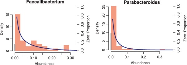
Examples of two genera from the real human microbiome data. Red bars represent the density of the non-zero data (left Y axis). Black bars represent the zero proportion (right Y axis). Back curves show the fit of the non-zero data using a Beta distribution

Our model considers each taxon separately. For each given bacterial taxon, let $Y_{it}\hspace{0.5em}(i=1,2,\dots ,N,t=1,2,\dots ,T)$ be its relative abundance for subject i at time t , where $0\le Y_{it}<1$ . We assume that

$$Y_{it}\mathrm{\sim }0\text{\hspace{0.5em}with\hspace{0.5em}probability\hspace{0.5em}}1-p_{it}$$ (1)

$$\mathrm{\sim }\text{Beta}({\mu }_{it}\varphi ,(1-{\mu }_{it})\varphi )\text{\hspace{0.5em}with\hspace{0.5em}probability\hspace{0.5em}}{p}_{it},$$ (2)

where the density function of the Beta distribution is parameterized as

$$f(y_{it};{\mu }_{it},\varphi )=\frac{\Gamma (\varphi )}{\Gamma ({\mu }_{it}\varphi )\Gamma ((1-{\mu }_{it})\varphi )}{y}_{it}^{{\mu }_{it}\varphi -1}{(1-y_{it})}^{(1-{\mu }_{it})\varphi -1}$$ (3)

with μ _it$(0<{\mu }_{it}<1)$ and $\varphi$$(\varphi >0)$ being the mean and dispersion parameters of the Beta distribution, respectively. The parameter p _it is the probability that the observation Y _it is generated from the Beta component. Figure 1 shows that the Beta distribution fits the non-zero values of the real data well. In addition, we let the probability p _it of the logistic component and the mean of the Beta component μ _it depend on the covariates through the logit link functions,

$$\text{logit}(p_{it})=\log \left(\frac{p_{it}}{1-p_{it}}\right)={\alpha }_0+X_{it}^T\alpha +a_i,$$ (4)

$$\text{logit}({\mu }_{it})=\log \left(\frac{{\mu }_{it}}{1-{\mu }_{it}}\right)={\beta }_0+Z_{it}^T\beta +b_i,$$ (5)

where α ₀ and β ₀ are intercepts, a _i and b _i are the individual-specific random intercepts, X _i and Z _i are the covariates that can be time-dependent and are not necessarily the same, and α and β are the corresponding vectors of the regression coefficients.

This model can be considered as a two-part model with a logistic component and a Beta component. The logistic component models the presence/absence of the taxon in the samples and the Beta component models the non-zero abundance of the taxon. A covariate can affect the microbiome composition in two different ways: (i) it affects the presence/absence of the taxon in the samples, which is modeled through the logistic regression part in the model; (ii) it affects the relative abundance when the taxon presents in the samples. This is modeled by the Beta regression in the model. The data observed are from a mixture of these two models. This model is flexible to allow that the covariates affecting the presence/absence of the microbial species are different from the covariates affecting microbial abundance.

If the data are measured at repeated times, the responses at different time points within a subject are expected to be correlated. The repeated measures Y _it ( $t=1,\dots ,T)$ on the same subject i share the same individual-specific random effects of a _i and b _i across different time points, which can be used to model such correlations and to account for multiple sources of variance. We only include the random intercepts in the model since such simple random intercepts are often adequate in practice to capture the longitudinal correlations ( Min and Agresti, 2005 ). However, it is easy to extend our model to include random slopes. The random effects are assumed to follow an independent normal distribution,

$$a_i\sim N(0,{\sigma }_1^2),b_i\sim N(0,{\sigma }_2^2).$$

The parameters can be estimated by the standard maximum likelihood estimation (MLE), where the likelihood function is given as

$$\begin{array}{l}L(\alpha ,\beta ,\varphi ,{\sigma }_1^2,{\sigma }_2^2)\\ ={\displaystyle \prod _{i=1}^N{\displaystyle {\int }_{-\infty }^{\infty }{\displaystyle {\int }_{-\infty }^{\infty }{\displaystyle \prod _{t=1}^T{(1-p_{it})}^{I(Y_{it}=0)}}}}}{[p_{it}f({\mu }_{it},\varphi )]}^{I(Y_{it}>0)}\\ \times g(a_i,b_i|{\sigma }_1^2,{\sigma }_2^2)\text{\hspace{0.17em}d}{a}_i\text{d}{b}_i,\end{array}$$

where p _it and μ _it are defined through the logistic regression models (4)–(5), $f({\mu }_{it},\varphi )$ is the Beta density function given in (3) and $g(a_i,b_i|{\sigma }_1^2,{\sigma }_2^2)$ is the product of two normal density functions.

To evaluate this likelihood function, we first integrate out the unobserved random effects to obtain a marginal likelihood. Since the integrals are analytically intractable, the marginal likelihood does not have a closed-form expression. We use Gauss-Hermite quadrature to approximate the integral by a finite sum. The MLE of $(\alpha ,\beta ,\varphi ,{\sigma }_1^2,{\sigma }_2^2)$ can be obtained numerically. The likelihood ratio test can be applied to test the following three biologically relevant null hypotheses:

• I the covariates are associated with the bacterial taxon by affecting its presence or absence, $H_0:{\alpha }_j=0$ ;

• II the taxon is associated with the covariates by showing different abundances, $H_0:{\beta }_j=0$ ;

• III the covariates affect the taxon both in terms of presence/absence and its abundance, $H_0:{\alpha }_j=0$ and ${\beta }_j=0$ for each covariate X _j and Z _j .

The P value can be obtained for each of these hypotheses. If the covariate X and Z are the same, the joint null (III) is $H_0:{\alpha }_j=0$ and ${\beta }_j=0$ , which tests the overall association between the covariate and the taxon abundance. We have implemented this model and the likelihood ratio tests as an R package ZIBR .

3 Simulation studies

To evaluate the performance of our proposed method ZIBR for longitudinal microbiome data, we carried out simulation studies first. We compared our method with the linear mixed-effects model with arcsine square root transformation (LMM) on the microbiome abundance as proposed in La Rosa et al. (2014) and Kostic et al. (2015) . LMM was compared since it was the only method that can jointly model data measured over all the time points in longitudinal microbiome studies.

We first evaluated the type I errors of the two methods. One binary covariate for both logistic and Beta components was used to mimic the case–control study design, where $X=Z=0$ for $\frac{1}{2}N$ subjects and $X=Z=1$ for the other $\frac{1}{2}N$ subjects. We set the regression coefficients as $\alpha =({\alpha }_0,{\alpha }_1)=(0,0),\beta =({\beta }_0,{\beta }_1)=(-0.5,0)$ , the variance of the mixed-effects as ${\sigma }_1={\sigma }_2=0.5$ and the dispersion parameter of the Beta distribution as $\varphi =5$ . These parameters were chosen to mimic the parameters estimated based on the real dataset analyzed in Section 4. The likelihood ratio test was performed to test the null hypothesis

$$H_0:{\alpha }_1={\beta }_1=0.$$

The simulation was carried out with different number of subjects ( N  = 50, 100, 150), each with T  = 5 time points. The simulations were repeated 10,000 times under each sample size setting. The type I error was calculated for two different nominal levels of 0.01 and 0.05.

The results are shown in Table 1 , indicating that both our proposed method ZIBR and LMM both controlled the type I errors reasonably well. We also evaluated the running time of ZIBR. It took 2.3, 4.0 and 7.0 s per simulation to run on a MacBook Pro laptop for sample size of N  =   50, 100, 150, respectively, indicating that the algorithm was very efficient.

Table 1.

Type I error for testing $H_0:{\alpha }_1={\beta }_1=0$ based on ZIBR and LMM for α-level of 0.01 and 0.05 for various sample sizes

	ZIBR	LMM	ZIBR	LMM
Sample size	0.01		0.05
N =50	0.0130	0.0107	0.0584	0.0484
N =100	0.0105	0.0096	0.0532	0.0507
N =150	0.0095	0.0100	0.0493	0.0494

Simulations were repeated 10 000 times.

We then evaluated the power of ZIBR for identifying the true association. We simulated 1000 bacterial species, of those, 400 were associated with the binary covariate and the rest, 600, were not associated. For each species, we simulated N  =   50 subjects with T  =   5 time points for each subject. We simulated the regression coefficients $({\alpha }_0,{\alpha }_1,{\beta }_0,{\beta }_1)$ either from a uniform distribution or set them to zero. Particularly, they were set to

1. $(-0.5,U(0.1,1),-0.5,U(0.1,1))$ for 100 species;

2. $(0.5,U(-1,-0.1),0.5,U(-1,-0.1))$ for 100 species;

3. $(-0.5,U(0.1,1),0.5,U(-1,-0.1))$ for 100 species;

4. $(0.5,U(-1,-0.1),-0.5,U(0.1,1))$ for 100 species;

5. $(0,0,-0.5,0)$ for 600 species.

Here scenarios (1) and (2) indicate that the associations in the logistic and Beta components have the same direction while scenarios (3) and (4) indicate different directions. Scenario (5) indicates no association in either logistic or Beta component. We simulated variance of the random effect as ${\sigma }_1\sim U(0.1,1),{\sigma }_2\sim U(0.1,1)$ and Beta dispersion parameter as $\varphi \sim U(2,10)$ . The performance of ZIBR and LMM were evaluated based on the receiver operating characteristic (ROC) curve for identifying the covariate-associated species. The ROC and area under the curve (AUC) analysis were performed using pROC package in R ( Robin et al. , 2011 ). The results are shown in Figure 2 . The AUC for ZIBR was 92.0 compared to 79.1 for LMM, showing a significant difference ( $P<2.2\times {10}^{-16}$ by DeLong’s test).

Fig. 2.

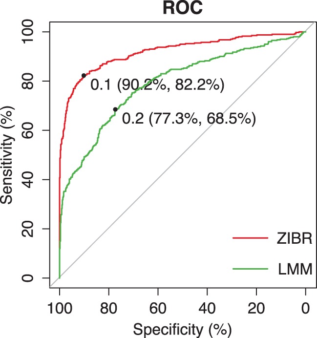
ROC curves for identifying association by ZIBR and LMM, where 1000 species were simulated and 400 of them had true association with the covariate. The simulations were carried out with N  = 50 subjects and T  = 5 time points for each subject. LMM is the linear mixed-effects model with arcsine square root transformation on the microbial abundance. The best cutoff and the corresponding specificity and sensitivity for each method are indicated, where the best cutoff is defined as the value such that the sum of sensitivity and specificity is the largest (Color version of this figure is available at Bioinformatics online.)

We also performed simulations to evaluate the power of ZIBR and LMM as a function of the proportion of zeros in the data as the value of α ₀ varied. The intercept α ₀ controls the proportion of zeros presented in the data. Four different parameter settings for $({\alpha }_0,{\alpha }_1,{\beta }_0,{\beta }_1)$ were considered, where α ₀ was evenly chosen from the above intervals to generate the power curves. The power curves are plotted in Figure 3 as the α ₀ value increases, which corresponds to decreased proportion of zeros presented in the data. Similar to the previous simulations, scenario (1) assumed that the associations in the logistic and Beta components had the same direction while scenario (2) implied different directions. Scenario (3) assumed no association in logistic component and scenario (4) assumed no association in the Beta component. In each scenario, we simulated N  =   50 subjects with T  =   5 time points for each subject. The covariates X and Z as well as ${\sigma }_1,{\sigma }_2,\varphi$ were simulated in the same way as in the previous simulations. The simulation for each α ₀ value was repeated 10 000 times. For ZIBR, we tested the null hypothesis $H_0:{\alpha }_1={\beta }_1=0$ with an α-level of 0.05.

Fig. 3.

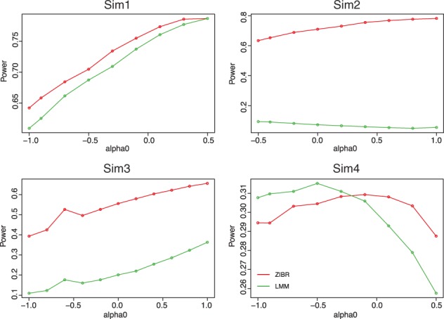
Power curves for identifying association by ZIBR and LMM. In each plot, the power was plotted against the α ₀ value, which controlled the proportion of zeros presented in the data, where a larger α ₀ value indicated smaller proportion of zeros presented in the data. Four different scenarios were simulated (see Section 3 for details). The simulation for each α ₀ value was repeated 10 000 times (Color version of this figure is available at Bioinformatics online.)

1. $([-1,0.5],0.5,0.5,0.5)$ ,

2. $([-0.5,1],-0.5,0.5,0.5)$ ,

3. $([-1,1],0,0.5,0.5)$ ,

4. $([-1,0.5],0.5,0,0)$ ,

As the proportion of zeros decreased in the data, the power of detecting the true association increased for both ZIBR and LMM except for scenario (4). Generally, ZIBR had greater power than LMM especially when the association in the logistic and Beta components had different directions [scenario (2)] or no association was assumed in logistic component [scenario (3)]. When the association in the logistic and Beta components had the same direction, ZIBR and LMM had the similar power [scenario (1)]. When the association was assumed only for the logistic component, the power of ZIBR and LMM decreased as the proportion of zeros in the data decreased.

4 Real data analysis

We applied ZIBR to a real microbiome study comparing different therapies for pediatric IBD patients ( Lee et al. , 2015 ; Lewis et al. , 2015 ). The study collected 90 children with IBD who received one of the three study therapies, including 52 children receiving anti-TNF, 22 receiving exclusive enteral nutrition (EEN) and 16 receiving partial enteral nutrition with ad lib diet (PEN). Adequate stool samples were available from 86 individuals to conduct shotgun metagenomic analysis. Gut microbiome samples were collected at four time points: baseline, 1 week, 4 weeks and 8 weeks into the therapy. The bacterial abundances at genus level were quantified using MetaPhlAn 1.7.6 ( Segata et al. , 2012 ). The low sequencing depth samples and low abundant genus were removed as in Kostic et al. (2015) , Romero et al. (2014) and Stein et al. (2013) . After filtering, we had a total of 236 samples with 59 subjects (47 anti-TNF and 12 EEN) and four time points for each subject as well as 18 most common bacterial genera. Our goal was to identify the bacterial genera that showed overall different abundances over three time points between EEN and anti-TNF treatments, adjusting for time effect and the abundance at the baseline. We fitted ZIBR with the baseline abundance, week and treatment as covariates and compared the results from fitting the linear mixed-effects model ( Kostic et al. , 2015 ; La Rosa et al. , 2014 ) with the same covariates and a subject-specific random effect. For the LMM, the relative abundance was arcsine square root transformed before fitting the model. The linear mixed-effects model was fitted using the lme function from nlme package in R. The P -values were adjusted using the Benjamini–Hochberg procedure to control the FDR.

At FDR = 5%, LMM identified seven genera, including Ruminococcus , Faecalibacterium , Bifidobacterium , Dialister , Streptococcus , Haemophilus and Alistipes . ZIBR identified all those seven genera and also identified four additional genera, Lactobacillus, Veillonella, Collinsella and Eubacterium ( Fig. 4 ). Table 2 shows the FDR-adjusted P -value for each of the three covariates in the model, indicating that the initial abundance of these four genera had large effects for their abundance during the course of the treatment. However, these genera were relatively stable in their abundance during the 8 weeks of treatments.

Fig. 4.

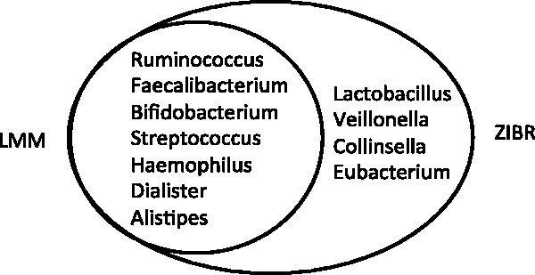
.Bacterial genera that showed different abundances between anti-TNF and EEN treatments identified by ZIBR and LMM after adjusting for the initial abundance. LMM identified seven genera, which were also identified by ZIBR. ZIBR identified four additional genera

Table 2.

Comparison of the results from ZIBR and LMM for four bacterial genera, where three covariates, including the baseline abundance, time and treatment, were included in each model

	LMM			ZIBR
Species	Baseline	Time	Treatment	Baseline	Time	Treatment
Lactobacillus	1.10E-11	5.68E-02	4.97E-01	2.46E-07	5.38E-01	9.41E-03
Veillonella	9.04E-07	8.04E-01	5.27E-01	4.81E-07	9.89E-01	1.76E-02
Collinsella	2.28E-07	9.85E-01	2.91E-01	6.14E-09	5.38E-01	1.57E-02
Eubacterium	1.03E-02	1.84E-02	5.04E-02	1.18E-02	2.43E-01	2.67E-02

For each genus, the FDR-adjusted P -value is shown for each of the three covariates in the model.

After adjusting the baseline abundance, these four genera showed different abundances between anti-TNF and the EEN treatments. Figure 5 shows the abundances of those four genera over time. Lactobacillus and Veillonella were observed more frequently in the anti-TNF-treated group across different time points than in the EEN group. However, no significant difference was observed for the non-zero abundance when they were observed. In contrast, Collinsella and Eubacterium showed consistent differences across all three time points in the non-zero abundance but not the frequencies being observed. Results from ZIBR showed that different treatments led to different probabilities of observing Lactobacillus and Veillonella (FDR-adjusted P  =   0.0049, FDR adjusted P  =   0.0085), but not Collinsella or Eubacterium (FDR-adjusted P  =   0.30, FDR-adjusted P  =   0.50). In addition, different treatments seemed to lead to different abundances for Collinsella and Eubacterium (FDR-adjusted P  =   0.025, FDR-adjusted P  =   0.025), but not for Lactobacillus or Veillonella (FDR-adjusted P  = 0.42, FDR-adjusted P  = 0.93). The advantage of ZIBR is that it considers these two types of differences simultaneously, and therefore, potentially leads to more power in detecting the differences in abundances between the two treatment groups.

Fig. 5.

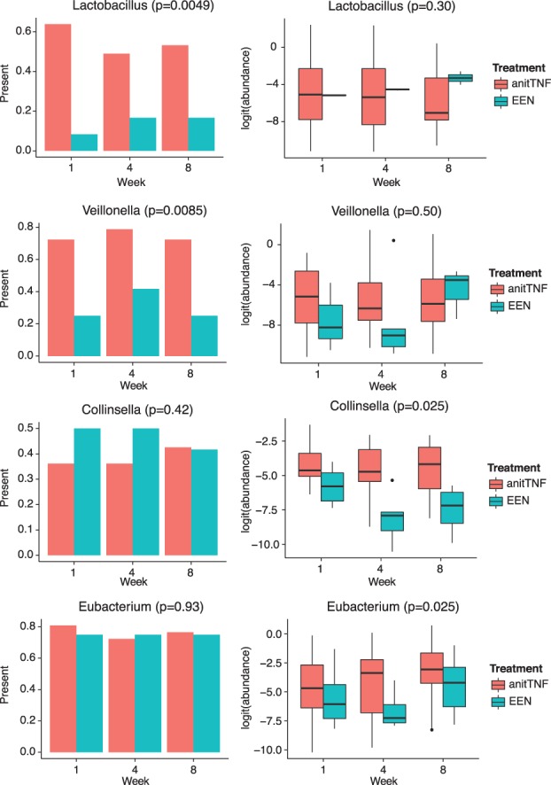
Four genera identified by ZIBR but not by LMM. Left panel shows the percentage of samples in EEN or anti-TNF groups where the genus was present. Right panel shows the non-zero abundance in EEN or anti-TNF groups, where the abundances were logit-transformed (Color version of this figure is available at Bioinformatics online.)

5 Discussion

We have proposed a two-part mixed-effects model to identify the taxa that are associated with clinical covariates in the longitudinal microbiome studies. Our model takes into account the compositional and sparse nature of the microbiome data as well as the correlations among the repeated measures in the longitudinal studies. We have demonstrated that our proposed model outperformed the commonly used linear mixed-effects models in identifying the covariates-associated taxa. We applied our method to a real human microbiome study of IBD treatment and identified a number of bacterial genera that showed different abundances between two commonly used treatments during the 8-week treatment period.

The model we proposed in this paper can be applied to proportion data obtained from either 16S rRNA sequencing or shotgun metagenomic sequencing. For shotgun metagenomic data, it is not clear how to summarize the sequencing reads into bacterial counts since many reads can be aligned to multiple bacterial genomes. Therefore, most commonly used methods such as MetaPhlAn only output the relative abundances or proportions of the bacteria in the sample. For 16S count data, methods developed for testing associations for RNA-seq count data such as DEseq ( Anders and Huber, 2010 ) and EdgeR ( Robinson and Smyth, 2007 ) have been applied to the microbiome studies ( McMurdie and Holmes, 2014 ). However, compared to RNA-seq data, 16S counts often include excessive zeros, which can violate the assumptions made for RNA-seq count data. To deal with the problem of excessive zeros, Paulson et al. (2013) developed a zero-inflated Gaussian model with the log-transformation on the read counts for 16S rRNA sequencing data, where an empirical Bayes procedure was developed to estimate the moderated variances. However, those methods are developed for 16S count data and thus not suitable for proportion data. In addition, it is not clear how to extend the empirical Bayes method of Paulson et al. (2013) to repeatedly measured count data. It is not trivial to extend these methods to simply include certain random effects.

The zero-inflated beta regression model ( Peng et al. , 2015 ) and zero-or-one inflated beta regression model ( Ospina and Ferrari, 2012 ) have been developed for proportion data. However, none of the methods can handle repeatedly measured proportion data such as the longitudinal data considered in this paper. The difference between these models and our model is that our model includes two random intercept terms in order to model the dependency of the data measured over time. This is important for analyzing longitudinal data since the observations are not independent. Including random effects also allows us to model multiple sources of variance that cannot be accounted for by the observed covariates.

The two-part mixed-effects regression model we proposed here is similar to what were studied in literature, e.g. zero-inflated Poisson, binomial and negative binomial regression with random effects ( Hall, 2000 ; Min and Agresti, 2005 ). In all these models, shared subject-specific random effect is included in the model in order to model the dependency of the observations across time. Our model [ Equations (4) and (5) ] allows two components to have different individual-specific random effects to allow for possible different dependency structures for the zero and non-zero parts of the data. These random effects are also used to account for multiple sources of variance. Our model does not assume that the correlation across time is purely caused by the covariates X and Z , it is the random effects that lead to the observed correlations across time.

One of the characteristics of the compositional data is the relative abundances of all taxa in the sample sum to one. Joint analysis of all the taxa needs to account for this unit sum constraint and several methods have recent been developed ( Li, 2015 ). However, in our application, each taxon is analyzed independently using the proposed ZIBR model and differential abundant taxa are selected by controlling the FDR. In such analyses, the sum-to-one constraint in the compositional microbiome data is not relevant. The unit sum of the data may lead to certain dependency the likelihood ratio statistics among the taxa, which may affect the performance of the FDR controlling procedure of Benjamini and Hochberg (1995) .

In our simulations and analysis of real data, the ZIBR model involves the same covariates for logistic regressions and Beta regression. However, our model is more flexible, which can include multiple covariates and different covariates in two different components of the model. Besides identifying bacterial taxa, the model proposed here can also be applied to identify microbial genes or pathways that show different profiles in longitudinal microbiome studies.

References

- Anders S., Huber W. ( 2010. ) Differential expression analysis for sequence count data . Genome Biol ., 11 , R106.. [DOI] [PMC free article] [PubMed] [Google Scholar]
- Arrieta M.C. et al. . ( 2015. ) Early infancy microbial and metabolic alterations affect risk of childhood asthma . Sci. Transl. Med ., 7 , 307ra152 – 307ra152 . [DOI] [PubMed] [Google Scholar]
- Bäckhed F. et al. . ( 2015. ) Dynamics and stabilization of the human gut microbiome during the first year of life . Cell Host Microbe , 17 , 690 – 703 . [DOI] [PubMed] [Google Scholar]
- Benjamini Y., Hochberg Y. ( 1995. ) Controlling the false discovery rate: a practical and powerful approach to multiple testing . J. R. Stat. Soc. Ser. B , 57 , 289 – 300 . [Google Scholar]
- Cox L.M. et al. . ( 2014. ) Altering the intestinal microbiota during a critical developmental window has lasting metabolic consequences . Cell , 158 , 705 – 721 . [DOI] [PMC free article] [PubMed] [Google Scholar]
- David L.A. et al. . ( 2014. ) Diet rapidly and reproducibly alters the human gut microbiome . Nature , 505 , 559+ . [DOI] [PMC free article] [PubMed] [Google Scholar]
- Faust K. et al. . ( 2015. ) Metagenomics meets time series analysis: unraveling microbial community dynamics . Curr. Opin. Microbiol ., 25 , 56 – 66 . [DOI] [PubMed] [Google Scholar]
- Gerber G.K. ( 2014. ) The dynamic microbiome . FEBS Lett ., 588 , 4131 – 4139 . [DOI] [PubMed] [Google Scholar]
- González A. et al. . ( 2012. ) Characterizing microbial communities through space and time . Curr. Opin. Biotechnol ., 23 , 431 – 436 . [DOI] [PMC free article] [PubMed] [Google Scholar]
- Hall D.B. ( 2000. ) Zero-inflated Poisson and binomial regression with random effects: a case study . Biometrics , 56 , 1030 – 1039 . [DOI] [PubMed] [Google Scholar]
- Koren O. et al. . ( 2012. ) Host remodeling of the gut microbiome and metabolic changes during pregnancy . Cell , 150 , 470 – 480 . [DOI] [PMC free article] [PubMed] [Google Scholar]
- Kostic A.D. et al. . ( 2014. ) The microbiome in inflammatory bowel disease: current status and the future ahead . Gastroenterology , 146 , 1489 – 1499 . [DOI] [PMC free article] [PubMed] [Google Scholar]
- Kostic A.D. et al. . ( 2015. ) The dynamics of the human infant gut microbiome in development and in progression toward type 1 diabetes . Cell Host Microbe , 17 , 260 – 273 . [DOI] [PMC free article] [PubMed] [Google Scholar]
- La Rosa P.S. et al. . ( 2014. ) Patterned progression of bacterial populations in the premature infant gut . Proc. Natl. Acad. Sci. U. S. A ., 111 , 12522 – 12527 . [DOI] [PMC free article] [PubMed] [Google Scholar]
- Lee D. et al. . ( 2015. ) Comparative effectiveness of nutritional and biological therapy in North American children with active Crohn’s disease . Inflamm. Bowel Dis . [DOI] [PubMed] [Google Scholar]
- Lewis J.D. et al. . ( 2015. ) Inflammation, antibiotics, and diet as environmental stressors of the gut microbiome in pediatric Crohn’s disease . Cell Host Microbe , 18 , 489 – 500 . [DOI] [PMC free article] [PubMed] [Google Scholar]
- Li H. ( 2015. ) Microbiome, metagenomics, and high-dimensional compositional data analysis . Annu. Rev. Stat. Appl ., 2 , 73 – 94 . [Google Scholar]
- Markle J.G. et al. . ( 2013. ) Sex differences in the gut microbiome drive hormone-dependent regulation of autoimmunity . Science , 339 , 1084 – 1088 . [DOI] [PubMed] [Google Scholar]
- McMurdie P.J., Holmes S. ( 2014. ) Waste not, want not: why rarefying microbiome data is inadmissible . PLoS Comput. Biol ., 10 , e1003531.. [DOI] [PMC free article] [PubMed] [Google Scholar]
- Min Y., Agresti A. ( 2005. ) Random effect models for repeated measures of zero-inflated count data . Stat. Modell ., 5 , 1 – 19 . [Google Scholar]
- Ospina R., Ferrari S.L. ( 2012. ) A general class of zero-or-one inflated beta regression models . Comput. Stat. Data Anal ., 56 , 1609 – 1623 . [Google Scholar]
- Paulson J.N. et al. . ( 2013. ) Differential abundance analysis for microbial marker-gene surveys . Nat. Methods , 10 , 1200 – 1202 . [DOI] [PMC free article] [PubMed] [Google Scholar]
- Peng X. et al. . ( 2015. ) Zero-inflated beta regression for differential abundance analysis with metagenomics data . J. Comput. Biol , 23 , 102 – 110 . [DOI] [PMC free article] [PubMed] [Google Scholar]
- Qin J. et al. . ( 2010. ) A human gut microbial gene catalogue established by metagenomic sequencing . Nature , 464 , 59 – 65 . [DOI] [PMC free article] [PubMed] [Google Scholar]
- Qin J. et al. . ( 2012. ) A metagenome-wide association study of gut microbiota in type 2 diabetes . Nature , 490 , 55 – 60 . [DOI] [PubMed] [Google Scholar]
- Robin X. et al. . ( 2011. ) proc: an open-source package for r and s+ to analyze and compare roc curves . BMC Bioinformatics , 12 , 77.. [DOI] [PMC free article] [PubMed] [Google Scholar]
- Robinson M., Smyth G. ( 2007. ) Small-sample estimation of negative binomial dispersion, with applications to sage data . Biostatistics , 9 , 321 – 332 . [DOI] [PubMed] [Google Scholar]
- Romero R. et al. . ( 2014. ) The composition and stability of the vaginal microbiota of normal pregnant women is different from that of non-pregnant women . Microbiome , 2 , 4.. [DOI] [PMC free article] [PubMed] [Google Scholar]
- Rutten N.B.M.M. et al. . ( 2015. ) Long term development of gut microbiota composition in atopic children: impact of probiotics . PloS One , 10 , e0137681.. [DOI] [PMC free article] [PubMed] [Google Scholar]
- Schulz M.D. et al. . ( 2014. ) High-fat-diet-mediated dysbiosis promotes intestinal carcinogenesis independently of obesity . Nature , 514 , 508 – 512 . [DOI] [PMC free article] [PubMed] [Google Scholar]
- Segata N. et al. . ( 2012. ) Metagenomic microbial community profiling using unique clade-specific marker genes . Nat. Methods , 9 , 811 – 814 . [DOI] [PMC free article] [PubMed] [Google Scholar]
- Stein R.R. et al. . ( 2013. ) Ecological modeling from time-series inference: insight into dynamics and stability of intestinal microbiota . PLoS Comput. Biol ., 9 , e1003388.. [DOI] [PMC free article] [PubMed] [Google Scholar]
- Turnbaugh P.J. et al. . ( 2006. ) An obesity-associated gut microbiome with increased capacity for energy harvest . Nature , 444 , 1027 – 1131 . [DOI] [PubMed] [Google Scholar]
- Turnbaugh P.J. et al. . ( 2007. ) The human microbiome project . Nature , 449 , 804 – 810 . [DOI] [PMC free article] [PubMed] [Google Scholar]
- Tyler A.D. et al. . ( 2014. ) Analyzing the human microbiome: a how to guide for physicians . Am. J. Gastroenterol ., 109 , 983 – 993 . [DOI] [PubMed] [Google Scholar]
- Wagner B.D. et al. . ( 2011. ) Application of two-part statistics for comparison of sequence variant counts . PloS One , 6 , e20296–e20296.. [DOI] [PMC free article] [PubMed] [Google Scholar]
- Zhou Y. et al. . ( 2015. ) Longitudinal analysis of the premature infant intestinal microbiome prior to necrotizing enterocolitis: a case-control study . PloS One , 10 , e0118632–e0118632.. [DOI] [PMC free article] [PubMed] [Google Scholar]