How Does Household Income Affect Child Personality Traits and Behaviors?

Abstract

We examine the effects of a quasi-experimental unconditional household income transfer on child emotional and behavioral health and personality traits. Using longitudinal data, we find that there are large beneficial effects on children’s emotional and behavioral health and personality traits during adolescence. We find evidence that these effects are most pronounced for children who start out with the lowest initial endowments. The income intervention also results in improvements in parental relationships which we interpret as a potential mechanism behind our findings.

Social scientists have spent a considerable amount of effort uncovering the theoretical and empirical linkages between family resources and human capital formation in children (Currie and Almond 2011; Cunha et al. 2006; Becker and Tomes 1986; Duncan and Brooks-Gunn 1997; Cameron and Heckman 1998; Blau 1999). Their findings suggest that the intergenerational transmission of disadvantage is closely related to factors determined by the household environment. Public policy intended to remedy this situation has often favored programs that counteract family characteristics and household practices via interventions delivered in institutional settings, such as a school or health clinic. A substantial literature has evaluated the effectiveness of these interventions; researchers have investigated Head Start, Perry Preschool Study, TN STAR program, the Abecedarian Project experiment in North Carolina, and the Jamaica Study.¹ These types of institution-based programs have been shown to increase scores on measures of personality traits and improve different types of behaviors all of which result in improved long-run outcomes for children.

What if it were possible to remediate deficits in the household environment directly at the household level independently from institution-based interventions? For instance, some studies have found a causal link between parental resources and children’s test scores, physical health in childhood, long-term educational attainment, and social outcomes (Duncan, Brooks-Gunn, and Klebanov 1994; Duncan et al. 1998; Duncan, Morris, and Rodrigues 2011; Shea 2000; Plug and Vijverberg 2003; Milligan and Stabile 2011; Akee et al. 2010). Research evaluating the effect of household income on child outcomes has shown that income interventions can have positive long-run effects on children’s health (Hoynes, Schanzenbach, and Almond 2016; Aizer et al. 2016; Hoynes, Miller, and Simon 2015). It is now clear that “nature” alone does not determine the well-documented underperformance of children from poor households. While unconditional income transfers appears to be a costly policy, the resulting improvements in child outcomes may provide significant long-run societal benefits that may justify the costs. Thus, income-enhancing programs that provide an alternative to institution-based programs are increasingly gaining favor among economists (Banerjee et al. 2015).

Existing studies have been able to show the link between increased household income and child health and labor market outcomes. However, the literature rarely presents evidence on the mechanisms behind the observed effects. It is clear how most institution-based interventions function to improve child outcomes due to, for example, smaller class sizes, increased health awareness, counseling, or improved parenting skills; the same cannot be said with any certainty about household-level cash-based interventions.

Our study allows us to peer into this black box at the household level and identify some of the mechanisms that translate extra household income into better child outcomes. We examine the effect of an unconditional cash transfer program on children using a longitudinal dataset. The Great Smoky Mountains Study (GSMS) covers a representative sample of children from 11 counties in North Carolina at ages 9, 11, and 13 at the beginning of the survey who were interviewed annually until age 16. Their parents were also interviewed in the same survey waves. There is an oversample of American Indian children in the GSMS. These American Indian households began to receive, five years into the initial survey, direct cash transfers from the Eastern Band of Cherokee Indians tribal government from the revenues of a new casino on their reservation.² These transfers are provided to all adult enrolled citizens of the tribe, regardless of employment conditions, marital status, presence of young children, or residence on the reservation. The longitudinal nature of the data allows us to investigate changes at the household level before and after the introduction of the unconditional cash transfers and compare those who receive them to households that never received the transfers. Furthermore, since the survey was primarily intended to collect data on behavioral and mental health, we have a wealth of information on the child’s emotional and behavioral well-being as well as a few measures for the parents.

This unique quasi-experimental setting enables us to make several contributions to the existing literature on the determinants of child well-being in the short run and into adulthood. First, we show that the increase in unconditional household income improves child personality traits, emotional well-being, and behavioral health. Because of the panel nature of the dataset, we can demonstrate these improvements within the same child and using the same measures over time. The formation of positive personality traits, such as conscientiousness and agreeableness, is crucial in determining long-term socioeconomic standing and may also have strong effects on long-term health, educational attainment, and economic outcomes (see, e.g., Almlund et al. 2011; Heckman, Pinto, and Savelyev 2013; Campbell et al. 2014; Cunha and Heckman 2008; Cunha, Heckman, and Schennach 2010).

There is a socioeconomic status (SES) gradient to this aspect of child well-being as well. Mental health conditions, such as attention deficit hyperactivity disorder and developmental delays, are more likely to affect poorer children (Currie and Lin 2007). Indeed, low SES might work as an early-life stressor that determines part or all of the relationship between low parental income and children’s mental health problems (see Lundberg 1997, McLeod and Shanahan 1993). To our knowledge, ours is the first study to examine the direct effect of changes in unconditional household income on personality traits and children’s mental health in a quasi-experimental framework (see review by Duncan, Magnuson, and Votruba-Drzal 2014). Our results suggest that the effect of an increase in household income on these important child characteristics is nontrivial among children first treated in their early teenage years.³

Second, we demonstrate that conscientiousness, agreeableness, and symptoms of emotional distress are malleable into the teenage years. While existing research suggests that personality traits may be plastic into late adolescence and even into young adulthood, most of the prior evidence on this point is based on observational studies.⁴ School-based interventions in early childhood, on the other hand, have shown quite conclusively that personality traits can be altered during childhood and these changes are predictive of adult outcomes (see, for instance, Gertler et al. 2014 or Heckman, Pinto, and Savelyev 2013).⁵ If income transfers are effective in improving emotional well-being into the adolescent years, as our findings suggest, then the window of opportunity and policy options available to break the intergenerational transmission of low SES are greater than previously thought.

Third, because of the panel nature of the survey data at the child level, our results are identified off within-child changes to behavioral and emotional distress symptoms, and personality traits. This allows us to net out any unobserved family-specific and child-specific factors that might confound the estimated treatment effects. Fourth, we can test for heterogeneous effects of the transfers across the initial distribution of the outcomes of interest. We find that the children that start out with the most severe personality or behavioral deficits are the ones who exhibit the greatest improvements.

Finally, the detailed nature of our survey data allows us to examine some of the potential mechanisms through which the additional unconditional household income affects child personality traits and behavioral disorders. We find that the unconditional cash transfers resulted in an improvement in parental mental health, the relationship between parents, and the relationship between the parents and children in the treated households. Thus, increases in household income may improve long-run child outcomes via the improvement in parental behaviors, stress-reduction, and improvements in decision making in the household. We are also able to rule out changes in marital status, changes in labor force participation, or full- or part-time employment as alternative explanations in this analysis.

Our results on mental health correspond to findings in the existing literature. The small literature on lottery winnings and mental health implies a small positive effect of a one-time positive income transfer on mental health (Lindahl 2005; Apouey and Clark 2015; Cesarini et al. 2014). Previous research has suggested that parents’ emotional and physical well-being are positively affected by increases in household income (Evans and Garthwaite 2014; Milligan and Stabile 2011; Jones, Milligan, and Stabile 2015). At the same time, McGue, Bacon, and Lykken (1993) suggest that changes in personality traits are due primarily to permanent changes in environment and Cunha and Heckman (2008) emphasize that parents have a large role in personality formation.

The next section discusses related literature, and we describe the data used in our analysis in Section II. We discuss the conceptual framework for our analysis in Section III and provide the empirical framework in Section IV. Section V presents the empirical results from our analysis, the potential mechanisms at work, and Section VI outlines several robustness checks. In Section VII we discuss our findings, their potential long-run effects for treated children, and conclude.

I. Related Literature

A. Identifying the Effects of Extra Income on Child Outcomes

Using the Fragile Families and Child Well-Being Study, Berger, Paxson, and Waldfogel (2009) find a strong correlation between measures of children’s mental health at age three, cognitive skills test scores, and family income. However, they also find a high correlation between other measures likely to affect child well-being (such as the physical environment in the home) and child outcomes. The presence of multiple correlates of child well-being and household conditions underscores the main difficulty in identifying the effect of family income on children. It is likely that a number of observable and unobservable variables are related to income and the outcome variable of interest. A number of recent papers have attempted to overcome this difficulty by using exogenous changes in policies or economic shocks to investigate how changes to household resources affect child development.

One branch of the literature focuses on exogenous changes to family income due to tax benefits or welfare increases. Milligan and Stabile (2011) find that child-specific tax benefits for Canadian households improve child achievement and health outcomes. Dahl and Lochner (2012) and Duncan, Morris, and Rodrigues (2011) show that better household financial standing leads to an improvement in achievement test scores for low-income children. One frequently cited caveat in generalizing these findings is that because Earned Income Tax Credit (EITC) and welfare programs affect mostly the bottom part of the SES distribution, these findings are not generalizable to the entire population. Such programs also require positive labor market earnings and usually lead to changes in labor market participation and earned income, so that the pure income effects are hard to disentangle from possible substitution effects (Currie 2009; Heckman and Mosso 2014).

A number of studies have examined the effects of a conditional cash transfer program in Mexico known as both Oportunidades and PROGRESA.⁶ Less is known about the impact of unconditional and permanent cash transfers. One example is the extension of pension benefits in South Africa. Case (2004) found that an unexpected increase in household economic standing due to pension extension in South Africa improved the self-reported health of the recipient and of the rest of the household, while Duflo (2003) reports an additional positive effect on child height and weight.

The evidence from advanced economies is limited. In the United States, the Opportunity NYC–Family Rewards program provided about $3,000 per year to poor families in New York City, which is about 13 percent of the treatment group’s initial household income. This conditional cash transfer program was found to have improved graduation rates for a subset of children who were already proficient readers. Overall, it reduced the incidence of family poverty and hardship (Riccio et al. 2013). Using a large dataset of lottery winners from Sweden, Cesarini et al. (2015) investigate whether unexpected exogenous money receipts affect child health and development. They find no indication of improvements in children’s health, schooling outcomes, or cognitive and noncognitive skills as measured for males in the Swedish Army draft exams.⁷ There are several important differences between our study and theirs. First, winning the lottery is a rare event and the resulting income is likely perceived as a one-time income shock, as opposed to the permanent and regular semi-annual cash transfer we examine. Second, the social safety net in Sweden is much better developed than in the United States and differences in children’s access to adequate health care and schooling across SES are much less pronounced. Further, despite the richness of Swedish registry data, their dataset does not contain variables that measure the quality of household relationships. Information on household relationships and attitudes can only be collected using survey instruments such as the GSMS. Last but not least, the measure of noncognitive skills in young males as assessed by the Swedish Army draft is substantially different from the more standard and general measures captured by the GSMS.⁸

In the United States, Akee et al. (2010, 2013) used the Great Smoky Mountain Study data to examine the effect of changes in household income on child educational attainment, arrests, and obesity. Increased income has a strong effect on reducing criminality and improving educational attainment for the initially poorest households. However, there are differences in effects for childhood obesity depending upon initial household income level. Aizer et al. (2016) study a much earlier period in the United States and find that acceptance into the Mother’s Pension program, which provided up to 25 percent increase in family income for eligible mothers, resulted in better education and health outcomes for the household’s children. In addition to the different time periods, a substantial difference between their study and ours is that only eligible single mothers were selected into the Pension program and that the program lasted for about three years.

B. Household Income and Parental Behaviors

One potential channel linking children’s behavioral health and household income is related to parental well-being. Recent studies have found connections between exogenous income receipts and parental physiological and psychological health. In the United States, increasing EITC receipts has been linked to an improvement in maternal mental and physical health (Evans and Garthwaite 2014), while studies of the increase in Canadian child care subsidies have revealed a decreased incidence of maternal depression (Milligan and Stabile 2011) and a general improvement in household environment (Jones, Milligan, and Stabile 2015). Wolfe et al. (2012) use tribal casino operations (not receipt of casino transfer payments) to predict household income for American Indians in the Behavioral Risk Factors Surveillance System data. They find that opening a casino is associated with a reduction in adult anxiety, which may also be related to children’s long-term well-being.

The corresponding literature in psychology is in favor of the Family Stress model, which posits that economic hardships lead to increased emotional distress and ultimately marital strife (Conger, Rueter, and Elder 1999). In a series of papers, Conger and coauthors report that marital stress due to economic hardship has led to poorer parenting and more difficulty in adolescent boys’ emotional development (Conger et al. 1992) and that the onset of economic hardship leads to worse parenting behaviors (Conger et al. 2002).

To our knowledge, ours is the first study that uses longitudinal data on both parents and children to demonstrate that children’s personality traits and emotional well-being respond positively to permanent unconditional cash transfers and that there are concurrent positive changes in the household environment related to parental strife.

II. Great Smoky Mountains Study of Youth: Design and Background

A. Dataset Creation

The Great Smoky Mountains Study of Youth (GSMS) is a longitudinal survey of 1,420 children aged 9, 11, and 13 years at the survey intake, who were recruited from 11 counties in western North Carolina. The children were selected from a population of approximately 20,000 school-aged children using an age-at-intake-cohort-based design.⁹ American Indian children from the Eastern Band of Cherokee Indians (EBCI) were oversampled for this data collection effort.

The EBCI tribal reservation is situated in 2 of the 11 counties within the study. The initial survey contained 350 American Indian children and 1,070 non-Indian children. Proportional weights were assigned according to the probability of selection into the study; therefore, the data are representative of the school-aged population of children in this region. Attrition and non-response rates across different survey waves were found to be equal across racial and income groups (Akee et al. 2010).

The survey began in 1993 and followed three cohorts of children (ages 9, 11, 13 at survey intake) annually up to the age of 16, and then reinterviewed them at ages 19, 21, 24, and 25. Both parents and children were interviewed separately up until (and including) the year when the child was 16 years old; interviews after that were conducted with the child alone. In Appendix Figure 1, we provide a table identifying the survey timing for all three cohorts across survey waves. Both American Indian and non-Indian children were surveyed across all survey waves. Individuals are interviewed regardless of where they are living (whether on their own, or still living with their parents). No child is dropped from the survey simply because they moved out of their parent’s home.

We find no statistically significant difference in attrition between the sample of Native American children and the rest of the surveyed individuals. American Indians comprise 24 percent of the sample in the very first survey wave and comprise approximately 27 percent of the sample at age 21. The interviewers were residents of the study area who received one month of training for the study. They were randomly assigned to families across survey waves. Two of the interviewers were Native Americans (one of whom was Cherokee). Families received $10 to complete the initial wave of the survey and the compensation has increased over time (Costello et al. 1997).

B. Quasi-Experimental Income Intervention

After the fourth wave of the study, a casino opened on the Eastern Cherokee reservation. The Eastern Cherokee tribal government manages the revenues from the casino. A portion of the profits is distributed on a per capita basis to all adult tribal members. Disbursements from the casino revenues are made every six months to all enrolled tribal citizens and are subject to US federal income taxes. There are no means testing or other requirements other than tribal citizenship in order to receive the payments. Individual tribal members are eligible for the transfer payments whether they reside on or off the reservation; cash transfers are based on tribal enrollment status only. Based on other tribes’ experiences with similar revenue programs, the unconditional transfers were perceived as a permanent increase in income, although its size could vary from year to year. We estimate the amount of change in household incomes for those that were eligible for the unconditional transfers to be approximately $3,500 on average per year during the study period.¹⁰ This amount is roughly comparable to established government cash assistance programs such as Temporary Assistance for Needy Families (TANF) or the Supplemental Nutrition Assistance Program (SNAP) (French 2009).¹¹ The size of the per capita unconditional transfer during the study period is nontrivial in absolute and relative terms. The average income of AI households in the first three (pre-casino) survey waves was $22,781, so the initiation of the casino transfer increased household income by almost 15.4 percent on average (which is also roughly similar to amounts for recent US-based conditional cash transfer programs such as the Opportunity NYC–Family Reward (Riccio et al. 2013)).¹²

C. Creation and Description of Personality Traits and Psychological Measures

The Great Smoky Mountains Study was designed to assess mental health and well-being in children. Survey questions were specifically created to identify symptoms of behavioral and emotional disorders. Questions on the survey align with standard definitions for diagnoses and disorders from the Diagnostic and Statistical Manual of Mental Disorders IV (DSM-IV) (American Psychiatric Association 2000). In extracting the measures of personality traits from the survey instrument, we rely on recent developments in the child psychology literature that argue in favor of a continuum of measures of personality traits (see, e.g., Almlund et al. 2011 and Krueger and Eaton 2010).¹³ Extreme values of these measures are considered psychopathologies and are used to diagnose emotional/behavioral disorders (Wiggins and Pincus 1989). Non-extreme values are considered character traits, such as agreeableness or conscientiousness, with some individuals displaying stronger traits than others. That is why survey instruments (such as the GSMS), designed to map onto the DSM-IV, can be used to provide measures of personality and construct indices of behavioral and emotional disorder symptoms within the same analytical framework. A volume edited by Robert Cloninger (1999) discusses the relationship between personality traits and psychopathologies, as measured via the DSM-IV.

Costello et al. (1997) provide evidence on the presence of initial psychiatric disorders in the first survey wave. We use the count of behavioral and emotional disorders as identified in the survey as outcome variables. Behavioral disorders are defined as any conduct, oppositional, or antisocial personality disorder as defined in the Diagnostic and Statistical Manual of Mental Disorders IV (DSM-IV). Emotional disorders are defined as any anxiety or depression symptoms. These are constructed based on two sets of survey questions: parents’ reported observed behavior of their children and the children’s responses to direct questions from the interviewers. We use the union of the answers given by parents and children: i.e., if either respondent’s answer indicates a symptom, that symptom is considered present. A larger value indicates greater or more frequent instances of the outcome variable (higher probability of psychiatric diagnosis, more behavioral problems, more emotional problems). The counts of behavioral and emotional symptoms have been standardized with mean zero and unit standard deviation across all individuals by age. We provide the summary statistics for these two outcome variables for the first survey wave aggregated across all age cohorts by American Indian status in Table 1; due to this aggregation the mean and standard deviations are not exactly 0 and 1.

Table 1.

Table of Means for Outcomes at Initial Survey Wave

	American Indian		Non-Indian		Tests of equality of means
	Mean	Standard deviation	Mean	Standard deviation	Diff. in means	SE of diff.
Number of children < 6 years old	0.486	0.781	0.289	0.866	−0.197	0.051
Average household income in first three survey waves ($)	22,781	13,893	35,624	26,283	12,842	1,131
Biological parents married	0.443	0.497	0.578	0.738	0.134	0.036
Behavioral disorders	−0.228	0.694	−0.212	0.812	0.015	0.046
Emotional disorders	−0.268	0.804	−0.027	1.295	0.241	0.060
Conscientiousness	0.207	0.998	0.091	1.373	−0.116	0.071
Agreeableness	0.043	1.289	−0.164	1.534	−0.207	0.089
Neurotic	0.160	1.040	−0.123	1.698	−0.282	0.080
Adequate supervision of mothera	1.963	0.240	1.972	0.257	0.009	0.017
Enjoyable activities with mothera	1.875	0.389	1.897	0.505	0.022	0.028
Full-time employed mother	0.574	0.495	0.575	0.744	0.001	0.039
Poor relationship between parents	0.343	0.475	0.443	0.752	0.099	0.037
Arguments with parents	3.553	14.864	4.687	15.260	1.134	0.960

Notes: The number of observations for non-Indians ranges between 884–1,015 due to missing information for some variables; the number of observations for American Indians ranges between 323–270 due to missing information for some variables. Means and standard deviations are weighted using sample probability weights.

^aOn a scale of 0 to 2, higher values indicates more supervision or enjoyable activities.

We use a number of questions contained in the GSMS data that align with the Big Five Measures of Personality, commonly referred to measures of “noncognitive skills” or “social skills” or “personality,” that have been used in the prior literature in economics. Three dimensions of the Big Five are well suited to the GSMS survey questions. They are (i) Conscientiousness: tendency to be organized, responsible and hardworking; (ii) Agreeableness: tendency to act in a cooperative and unselfish manner; (iii) Neuroticism (also called Emotional Stability): chronic level of emotional instability and prone to psychological distress. The two remaining dimensions of the Big Five that we cannot measure with our data are Extraversion and Openness. Extraversion is intended to capture qualities such as the ability to inspire people, preference for human contact, empathy, and assertiveness. Openness to experience is a general tendency to engage in bold ideas and experiences, exhibit a high level of curiosity and adventure.¹⁴

Using data from the GSMS survey questionnaires, we found comparable questions which are similar to those that have been used in the determination of Conscientiousness, Agreeableness, and Neuroticism as personality traits in the existing economics literature. For these sets of questions, we only use answers from the parents. Self-reported answers may be unreliable at certain ages for adolescents.¹⁵ The full set of survey questions that were used to determine the three subparts of the Big 5 Personality traits are listed in Appendix Table 1.¹⁶ We recoded the personality trait measures so that a higher score indicates an increased intensity of one of the Big 5 personality traits (more conscientious, more agreeable, more neurotic). Thus an increase in a personality trait would be reflected in an increase of the measured level of the trait, while a deterioration in personality traits will be reflected in a decrease in the measured level of the trait. This positive association holds for conscientiousness and agreeableness; however, excessive increases in neuroticism can be classified as a pathology and a large increase in this trait is not necessarily a beneficial outcome.

Once we assembled those questions, we used principal component analysis, a method of multidimensional scaling. The method involves taking a linear transformation of a number of variables to reduce the number of dimensions (variables) to one. We retain the eigenvectors from the covariance matrix of all of these variables and use them to weight the contribution of each variable to the new (single dimensional) index; variables which contribute most are weighted more heavily in this index. Others have used variants of this method to create indices from survey questions in order to label the underlying indices of personality traits (Heckman, Pinto, and Savelyev 2013). We discuss the methods to create the personality traits indices in more detail in Appendix Section D.

Comparing our measures to those used by others in the literature reveals that they have similar correlations with income, educational attainment, and the child’s own age. In Appendix Table 2, we provide correlations between personality traits and several related SES outcomes estimated using our definitions and sample, as compared to what has been reported in other published work. Overall, the correlations we find are similar to what has been reported in other studies using different survey instruments to extract measures of personality.

Finally, we use a set of GSMS questions to construct variables measuring the quality of parental relationships and parental behaviors. These variables are measured in categories and increasing values indicate either better outcomes or improved relationships. Only one parent (the primary caregiver) is asked about the quality of the relationship between the parents. The child is asked whether they enjoy time spent with their mothers. A question about the number of arguments with children is asked of the primary caregiver only and is a count variable for the past three months. The data also include information regarding parental supervision. We describe these variables in Table 1.

Before the introduction of the unconditional transfers, American Indian households received about $13,000 less in annual income as compared to the rest of the sample. Income is recorded in $5,000 bins in the original data. We have transformed the categorical variable into a continuous variable in dollar terms in this table and subsequent analysis by multiplying income values in the respective bins by $5,000. American Indian households were more likely to have children younger than 6 and the parents were less likely to be married. American Indian children were somewhat less likely to report emotional problems and had higher levels of agreeableness, but they were also scored higher on neuroticism compared to the rest of the sample. Costello et al. (1997) report that the prevalence of psychiatric disorders in the survey population at baseline was in line with what was found in other epidemiological studies of similarly-aged children in the United States.

Appendix Table 3 summarizes data from several additional sources to demonstrate comparability of the American Indian population sampled in the GSMS to other demographic groups in the United States. The first two columns show summaries of characteristics for the Eastern Band of Cherokee Indians who resided on the tribal reservation for 1990 that allow us to compare them to the residents of the 11 counties in the GSMS study area. The tribal reservation residents were poorer on average by about $10,000, which is close to the income difference we find in the GSMS, and have comparable home ownership, marital status, and proportion of adults with a high school degree. The American Indians have almost double the unemployment rate of the 11-county average.

The next five columns compare the survey respondents to other disadvantaged minority groups and the rest of the United States using the 1990 IPUMS 1 percent sample (Ruggles et al. 2015). Median family income is similar for EBCI and other Native Americans while average family size is slightly smaller for the EBCI. Home ownership, marital status, and high school degree completion are similar across the three groups. The EBCI have a slightly lower unemployment rate and lower per capita income than the other two groups of Native Americans. The next column provides descriptive statistics for the rural African American population, the minority group most likely to exhibit similar characteristics to rural American Indians. There are many similarities with regard to income levels, home ownership, and unemployment levels as compared to the EBCI. However, rural African Americans have larger family sizes and lower high school degree completion rates. The final column provides the comparable data for the United States as a whole. Even though in 1990 the EBCI were clearly very economically disadvantaged compared to the average person in the United States, their socioeconomic standing was similar to that of other American Indians and African Americans residing in rural areas.

III. Conceptual Framework

A. Effects of Exogenous Income Shocks on Child Well-Being

Models of returns to investment in children generally build on Becker and Tomes (1979) and study how exogenous changes in the returns on child endowments affect parental behaviors and investments. Heckman (2007), Cunha and Heckman (2008), and Cunha, Heckman, and Schennach (2010) develop a model that allows for dynamic complementarities in skills across different periods of child development and has testable predictions about the shape of the production function for human capital. These models predict that a pure income effect would improve parental investments in children as long as children are viewed as normal goods.

Using our data in the pre-intervention period, we first confirm that there is a strong positive relationship between initial household income and initial personality skill endowment across both racial groups. The positive correlation between household income and child personality traits holds for American Indian children and non-Indian children alike and is suggestive evidence in favor of the predictions from the existing models cited above. In Appendix Figure 2, we provide the initial distribution of two of our outcome measures by initial household income using data prior to the income intervention. Conscientiousness varies positively with initial household income for both American Indian and non-Indian children. Emotional disorders vary inversely with initial household income levels prior to the casino intervention. Both results indicate that income has a direct relationship with both types of measures for American Indians and non-Indians prior to the casino operations.¹⁷ Notably, the income gradients in both measures are similar across racial groups. These figures, however, illustrate simple correlations and do not imply causality. We exploit the quasi-experimental setting of the cash transfers to gauge whether these associations remain when households receive exogenous increases in income.

A related conceptual question is whether there are any heterogeneities in the effect of an increase in this type of income across children with initially differing levels of personality traits and behavioral problems. Specifically, does the initiation of unconditional cash transfers have a differential effect depending upon the initial endowment of the child? If skill begets skill and assuming that families spend the extra income in a similar fashion, then we would expect that children with the largest skill endowment would benefit the most from the cash transfer program. On the other hand, if we see the most initially disadvantaged children catching up after the income transfers begin, then there is evidence of decreasing marginal returns to extra household income in the production of child personality traits and behaviors. Currie and Almond (2011) discuss this possibility using Heckman’s (2007) human capital accumulation model. A similarly-sized income shock could have a larger effect on households that have initially lower human capital investment. The authors note that the difference in the size of effects would be due to those households being on the steeper portion of the human capital production function.

The prediction from this model would be that children from households with lower initial investments in child skills would exhibit greater human capital gains from an increase (shock) in unconditional household income. Thus, both findings (that the best off or the worst off will realize the most benefits from the increase in household incomes) are conceptually possible. Our empirical methodology specified in the next section details our efforts to empirically distinguish between these two potential outcomes.

B. Identifying Mechanisms Affecting Child Outcomes

Our analysis also sheds some light on the mechanisms responsible for improving child outcomes. It is not immediately clear why an increase in household income would improve the conditions for underperforming children. For instance, if the poor are poor due to bad choices or preferences, then providing them with additional income alone will not necessarily achieve any observable improvements in their parenting and thus in children’s outcomes. If this is the case, then institution-based interventions may be more justified in order to improve child outcomes. On the other hand, if household income is a binding constraint for parental behaviors or household environment in general, then a relaxation of the budget constraint should produce observable improvement in child outcomes.

We directly test whether extra income results in changes in parental behaviors or household characteristics that may play a role in explaining the observed child improvement. We hypothesize that the increase in income provides a base level of income for treated households and helps to reduce financial strife within households. Existing research supports this hypothesis in a number of situations where incomes have been increased for parents in a quasi-experimental manner (Evans and Garthwaite 2014; Milligan and Stabile 2011; Jones, Milligan, and Stabile 2015; Conger, Rueter, and Elder 1999; Wolfe et al. 2012).

First, we examine whether the casino payment has an effect on parental behavior and quality of home life. Second, we measure whether the casino transfers affect marital status or parental employment. These measures are directly related to the conditions within the household. Finally, we provide evidence that other tribal government programs or American-Indian-specific programs are unlikely to be responsible for the observed change in child outcomes.

IV. Empirical Methodology

Our goal is to identify the effect of an unconditional cash transfer on child personality traits and behavioral and emotional disorder symptoms. Thus, our treatment will be referred to as either “cash transfer treatment” or the “casino treatment” and it indicates having lived in a household that received the unconditional cash transfers up to (and including) age 16.¹⁸

In this section, we describe our methodology which is based on a triple difference regression specification. However, it is useful to first discuss the foundations of this analysis via the various combinations of difference-in-differences analyses that are possible with our data. Given the cohort nature of the individual panel data, there are several approaches to setting up a difference-in-differences estimation. We discuss each of the possibilities below and conclude with our preferred triple difference specification.

One version of the difference-in-differences setup is to restrict the analysis to American Indian children only and exploit variation in the casino treatment across the three age cohorts. We observe the two youngest age cohorts (age 9 and age 11 at survey intake) residing in households that receive the unconditional transfers for 4 and 2 years, respectively, by the time they turn 16; the oldest cohort of children who were 13 years old at survey intake were not exposed to unconditional transfers by age 16. The identification of the cash transfer effect in this case would rely on the assumption that there are no significant time effects that could bias the estimated coefficients, as the estimated treatment effect would be also picking up any differences in child outcomes between for example the years 1995 and 2000 (comparing the youngest and oldest cohorts at the same age).

Second, we could restrict the sample by cohort and compare American Indian and non-Indian children across time. The assumption here would be that non-Indian children provide an adequate control group for American Indian children of the same age. If the progression of the outcome variables of interest was different among the non-Indian children, the estimated “treatment” effect would be picking up this difference.

A third possible cut of the data is to consider only children of the same ages, and compare outcomes across American Indian and non-Indian children using all cohorts. The identification in this case would come from differences in the cash transfers treatment across cohorts and race within the same age group. The important assumption is that there are no cohort-specific unobserved differences that would confound the coefficient of interest.

We present estimates from the three difference-in-differences frameworks as described above in Table 4. We also provide placebo regressions. The placebo regressions are intended to provide an empirical test of the main assumptions behind the respective difference-in-differences estimation.

Table 4.

Difference-in-Differences Analyses for Various Subgroups

		Behavioral disorder symptoms (1)	Emotional disorder symptoms (2)	Conscientiousness (3)	Agreeableness (4)	Neuroticism (5)
Panel A
Age 15–16 year olds only	Receipt of cash transfer	−0.263 (0.0791)	−0.0686 (0.111)	0.299 (0.0989)	0.301 (0.119)	0.148 (0.106)
	Observations	2,237	2,237	2,005	1,978	2,027
	R2	0.021	0.020	0.062	0.033	0.020
Panel B
Youngest age cohort alone	Receipt of cash transfer	−0.362 (0.153)	−0.565 (0.188)	0.428 (0.216)	0.208 (0.222)	0.481 (0.261)
	Observations	2,698	2,698	2,495	2,419	2,482
	R2	0.026	0.021	0.058	0.065	0.044
Panel C
American Indians alone	Receipt of cash transfer	−0.355 (0.195)	−0.191 (0.198)	0.391 (0.232)	0.773 (0.284)	0.334 (0.300)
	Observations	1,591	1,591	1,494	1,450	1,494
	R2	0.021	0.010	0.019	0.034	0.012
Panel D
Age 12–13 year olds only: placebo	Receipt of cash transfer	−0.0871 (0.101)	0.0663 (0.103)	0.0810 (0.129)	0.121 (0.130)	−0.245 (0.125)
	Observations	1,687	1,687	1,638	1,567	1,637
	R2	0.017	0.019	0.021	0.044	0.047
Panel E
Oldest age cohort alone: placebo	Receipt of cash transfer	0.147 (0.167)	−0.226 (0.173)	−0.306 (0.205)	0.221 (0.216)	−0.0241 (0.241)
	Observations	1,432	1,432	1,371	1,317	1,370
	R2	0.017	0.019	0.015	0.052	0.038
Panel F
Wave 4 observations only: placebo	Receipt of cash transfer	−0.118 (0.0974)	0.0468 (0.101)	0.174 (0.135)	0.0731 (0.131)	0.0254 (0.0977)
	Observations	1,109	1,109	1,068	1,024	1,078
	R2	0.004	0.010	0.018	0.008	0.006
Panel G
Non-Indians alone: placebo	Receipt of cash transfer	0.203 (0.139)	0.0369 (0.117)	−0.0358 (0.158)	0.383 (0.159)	0.229 (0.173)
	Observations	5,083	5,083	4,815	4,634	4,804
	R2	0.011	0.013	0.031	0.055	0.041

Notes: Panels A and D contain controls for treatment age groups, American Indian parents, SurveyWave fixed effects, number of children under six years old in the household, and a constant. Panel B and panel E contain controls for American Indian parents, age fixed effects, number of children under six years old in the household, and a constant. Panel F contains dummies for treatment age groups, American Indian parents, wave fixed effects, number of children under six years old in the household, and a constant. Panels C and G contain dummies for treatment age group, American Indian parents, age fixed effects, number of children under six years old in the household, and a constant. Standard errors clustered at the individual level.

A drawback in using only a difference-in-differences methodology in this setting is that in each case we are restricting the estimation to specific subsets of the data. Our preferred specification, a triple difference, uses all available data and all possible sources of variation in the data. In our analysis we compare outcomes across American Indians and non-Indians over time as well as across different age cohorts.¹⁹ The treatment effect is identified as the difference-in-differences-in-differences across age cohorts and race. The main estimating equation is

$$Y_{it}={\alpha }_0+{\beta }_1{\mathit{\text{YoungestCohorts}}}_i+{\beta }_2{\mathit{\text{After}}}_t+{\beta }_3{\mathit{\text{AmericanIndian}}}_i+{\delta }_1\mathit{\text{YoungestCohorts}}{s}_i\times {\mathit{\text{After}}}_t+{\delta }_2\mathit{\text{YoungestCohorts}}{s}_i\times {\mathit{\text{AmericanIndian}}}_i+\lambda \mathit{\text{YoungestCohorts}}{s}_i\times {\mathit{\text{After}}}_t\times {\mathit{\text{AmericanIndian}}}_i+X^{\prime }\mu +{\epsilon }_{it}.$$ (1)

In this equation, the subscript i denotes an individual child and the subscript t denotes a year (identical to survey wave). The coefficient of interest is λ. We control for all level effects by including indicator variables for survey waves, a dummy for American Indian race and indicators for the various cohorts. YoungestCohorts indicates that the child belonged to the youngest (age 9 at intake) or the second youngest (age 11 at survey start cohorts. The indicator variable After is equal to 1 from survey wave five onward, which is the period after the start of the casino transfer payment. We also include the double-interaction terms AmericanIndian × YoungestCohorts and YoungestCohorts × After with coefficients δ₁ and δ₂ The third double interaction term, After × AmericanIndian is omitted. All American Indian children are treated to the cash transfers at the same time and only the two youngest cohorts are observed after the cash transfer begins; thus, it is not possible to separately identify the coefficient on this double interaction from the triple interaction effects.

The psychology literature suggests that there are age-trends in child development. To account for this we include in the vector X a control for child age and the interaction between age and American Indian race. The vector X also includes calendar-month-specific dummies to account for any unobserved differences correlated with the timing of the survey interview. The vector X also includes a count variable for the number of children younger than six in the household.

To conduct the event-study analysis, we substitute the main interaction variable of interest in (1) AmericanIndian × YoungestCohorts × After with separate interaction dummies for each survey wave, AmericanIndian × YoungestCohorts × SurveyWave, and plot the coefficients on these indicator variables to graphically present the progression of the outcomes of interest over the entire window of observation from three years before treatment starts to four years after treatment.

The panel nature of the data allows us to include individual-specific fixed effects in equation (1). The estimates from these specifications rely on within-child changes in the outcomes of interest, net of any unobserved child-specific characteristics. The results from these models are very similar.

Proper identification of the treatment effect of the unconditional transfers depends on the assumption that the pre-trends for the dependent variables prior to the intervention are similar across treated and untreated groups.²⁰ Appendix Figure 3 tests for differences in the pre-casino trends for the five outcome variables for American Indian children and non-Indian children. The figure plots the coefficients and confidence intervals on interaction variables between year dummies (identical to survey waves) and child treatment status in (1). These five figures indicate that the trends across American Indians and non-Indians are not statistically significantly different across the first three survey waves.

Throughout the main analysis, we cluster the standard errors on the individual child level. Appendix Section C discusses and demonstrates the results from alternative approaches to estimating the standard errors. These alternative methods of estimating standard errors do not change the interpretation of our results.

V. Empirical Results

A. Main Effects of Income Intervention on Child Personality Traits and Behaviors

We start by documenting the effect of the unconditional transfers on household income. In Figure 1 we plot the coefficients on the SurveyWave × YoungestCohorts × AmericanIndian interaction terms in the triple difference specification. The omitted wave is survey wave 4, which happens in the year when the casino first opened. All other coefficients are estimated relative to this omitted category. While we see no significant differences in average income before the casino opens, there is an increase in the household income for American Indian households receiving the casino transfers in the years following the onset of the transfers. The amount is increasing in size over time; confirming anecdotal evidence that the size of the transfers was directly related to the casino revenues and was growing as the operations expanded over time.

Figure 1.

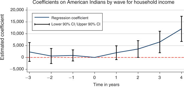
The Effects of Unconditional Transfers on Income around the Start of Casino Operations

Table 2 shows the estimates from the average treatment effects from the triple difference specification and the event-study results. In the first column of Table 2 we find that during the unconditional transfer period average annual income increased by about $3,500. Column 2 provides the estimated coefficients shown graphically in Figure 1.

Table 2.

The Effects of Casino Transfers on Household Income

	Total household income (1)	Total household income (2)
Receipt of cash transfer	3,472 (1,624)
SurveyWave 1 × YoungestCohorts × AI		2,309 (2,416)
SurveyWave 2 × YoungestCohorts × AI		595.1 (1,936)
SurveyWave 3 × YoungestCohorts × AI		850.8 (1,422)
SurveyWave 4 × YoungestCohorts × AI		Omitted category
SurveyWave 5 × YoungestCohorts × AI		1,996 (1,774)
SurveyWave 6 × YoungestCohorts × AI		3,550 (2,149)
SurveyWave 7 × YoungestCohorts × AI		6,527 (2,758)
SurveyWave 8 × YoungestCohorts × AI		12,055 (3,228)
Individual fixed effects	N	N
Observations	6,674	6,674
R2	0.077	0.078

Notes: Receipt of cash transfer is the triple difference coefficient from our empirical specification in (1). It is an interaction of American Indian × YoungestCohorts × After Casino. Casino payments began after wave 4 for only American Indian children. All regressions include secondary interaction variables American Indian × Cohort and Cohort × SurveyWave (indicators) and the main variables. They also include the number of children younger than 6, controls for child age and age interacted with American Indian race, year and month of interview controls, and a constant term. In column 2, Survey Wave Interaction variables are the interactions of American Indian × YoungestCohorts with each individual wave dummy variable. Income is coded in $5,000 income bins in the survey. For ease of interpretation, we transform the categorical variable into a continuous variable and present all amounts adjusted to 2000 US dollars. Standard errors clustered at the individual level.

The average number of dependent children in households receiving the unconditional transfers was 2.8. Therefore, the average household received about $1,250 per dependent child on average per year. We do not have information about how the households spent the cash, but given the low initial income levels in this group it is reasonable to assume that the money was spent, rather than saved or invested.

We provide similar event-style analysis in Figure 2 for the five outcome variables of interest; Appendix Table 5 provides the corresponding regression output that was used to create these figures. The five outcome variables are: behavioral disorder symptoms, emotional disorder symptoms, conscientiousness, agreeableness, and neuroticism. The first two figures show the effects of the casino transfer payments on behavioral and emotional disorder symptoms by year relative to the casino opening. To ease interpretation across different outcomes, these two outcome variables are normalized to mean zero and standard deviation of 1 across all individuals by age. There is a clear downward trend in the prevalence of these symptoms among the affected children after the advent of the transfers.

Figure 2.

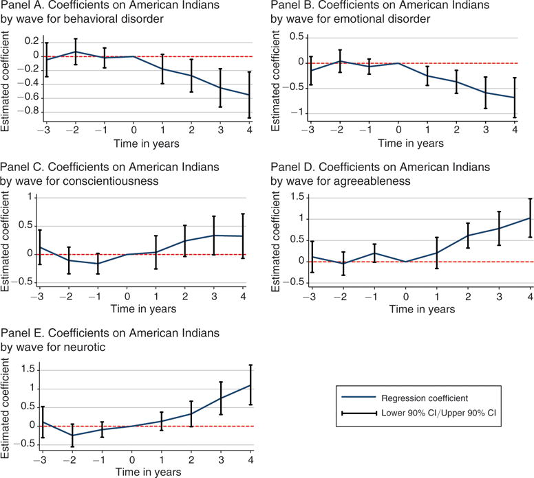
The Effects of Casino Transfers on Child Personality Traits and Behaviors around the Start of Casino Operations

The next three figures provide the corresponding plots for the personality traits. These three personality traits take on both positive and negative values and have mean zero. The outcome variables have been coded so that positive values indicate a higher intensity of the personality trait. There is an increase in the intensity of these traits for all three of the measures although they are of varying degrees of statistical significance across the survey waves.²¹

In Table 3 we provide the regression results showing the average treatment effect estimated using our specification in equation (1). Panel A shows the results without including person-specific fixed effects. Panel B reports the estimates from specifications in which we account also for child-specific fixed effects. The first two columns report effects of the casino transfers on the presence and severity of behavioral and emotional disorder symptoms observed in the child. The coefficient on the treatment variable implies a reduction in the number of behavioral disorder symptoms by 23 percent of a standard deviation. The estimates in the second column imply that the transfers reduced the incidence of emotional disorder symptoms for treated children by 37 percent of a standard deviation.

Table 3.

The Effect of Casino Transfers on Children’s Emotional and Behavioral Disorder Symptoms and Personality Traits

	Behavioral disorder symptoms (1)	Emotional disorder symptoms (2)	Conscientiousness (3)	Agreeableness (4)	Neuroticism (5)
Panel A
Receipt of cash transfer	−0.233 (0.104)	−0.374 (0.104)	0.254 (0.128)	0.374 (0.147)	0.381 (0.141)
Individual fixed effects	N	N	N	N	N
Mean of dependent variable	0	0	0	0	0
Standard deviation of dep. variable	1	1	1.221	1.390	1.454
Observations	6,674	6,674	6,309	6,084	6,298
R2	0.025	0.027	0.049	0.068	0.046
Number of individuals	1,420	1,420	1,414	1,404	1,413
Panel B
Receipt of cash transfer	−0.183 (0.0910)	−0.306 (0.102)	0.200 (0.121)	0.292 (0.146)	0.311 (0.137)
Individual fixed effects	Y	Y	Y	Y	Y
Mean of dependent variable	0	0	0	0	0
Standard deviation of dep. variable	1	1	1.221	1.390	1.454
Observations	6,674	6,674	6,309	6,084	6,298
R2	0.030	0.025	0.045	0.075	0.048
Number of individuals	1,420	1,420	1,414	1,404	1,413

Notes: For panels A and B, receipt of cash transfer is the triple difference coefficient from our empirical specification. It is an interaction of American Indian × YoungestCohorts × After casino. Casino payments began after wave 4 for only American Indian children. All regressions include secondary interactions American Indian × Cohort and Cohort × SurveyWave (indicators) and dummies for wave, cohort, and American Indian, as well as the number of children less than age 6 living in the household, controls for child’s age and the interaction of age with American Indian race, year and month of interview controls, and a constant term. Panel B includes the same controls as in panel A and also individual-specific fixed effects. Standard errors clustered at the individual level.

The next three columns provide the results for personality traits. The results indicate that the increase in household income has a positive effect on child personality traits. The unconditional cash transfer increases conscientiousness by almost 21 percent of a standard deviation; the effect of agreeableness is an increase of 27 percent of a standard deviation. These are substantial positive developments in the progression of these traits. Neuroticism also increases by 26 percent of a standard deviation. It is difficult to perfectly assign the results for neuroticism as purely good or bad: some traits that go into neuroticism may have a positive connotation, while some definitely do not. Thus, we note the positive (increasing) direction of the treatment effect but we cannot definitively interpret it as a purely positive or a purely negative development.

All of these estimates are slightly reduced in size but remain economically and statistically significant in the respective fixed effects specifications as reported in panel B (the coefficient on conscientiousness barely misses statistical significance at the 10 percent level). Overall, Table 3 shows consistent evidence that the unconditional cash transfers improve adolescent personality traits and reduce behavioral and emotional disorder symptoms. All standard errors are clustered on the individual child level. In Appendix Section C we present alternative approaches to estimating the standard errors. The results remain unchanged.

An important take-away from these findings is that personality traits and behavioral and emotional disorder symptoms can be affected by public interventions as late as the adolescent years. This confirms prior findings in economics (McCrae and Costa 1994; Heckman 2007; Borghans et al. 2008; Cunha, Heckman, and Schennach 2010; Morey and Hopwood 2013) and supports recent research in neuroscience that has found that the prefrontal cortex (the region of the brain which controls emotions and regulation) remains malleable into young adulthood (Dahl 2004).

Difference-in-Differences Analyses

Our preferred set of analyses relies on specification (1). In this subsection we provide estimates from various difference-in- differences models that help highlight the sources of the underlying variation. We complement the analysis with placebo tests that demonstrate that the variation driving our results is due to changes in the treated group rather than concurrent changes in the control groups.

Table 4 displays the estimates. Panel A restricts the analysis to children of age 15 or age 16. The estimation relies on differences across treated and untreated cohorts of American Indians and non-Indians at these ages. American Indian households with children in the youngest two cohorts were receiving the transfers when these children were aged 15 and 16. The oldest cohort of American Indian children’s households only started receiving the transfers when these children were 17. The main assumption behind this analysis is that cohort-specific effects are similar across American Indians and non-Indians. We find that the individuals from households that received the tribal government cash transfers experienced a reduction in behavioral and emotional disorder symptoms and an increase in conscientiousness and agreeableness at ages 15–16.

In panel B we report results for the youngest age cohort alone. American Indian children from this cohort were treated to the unconditional transfers for four years during the observation window. The non-Indian children are the control group. The comparison in this setup is across race and survey wave. The identifying assumption is that non-Indians serve as appropriate controls for the American Indians of the same age. We find effects similar to our triple-difference analyses; in unreported analysis we find qualitatively similar results when we use only observations from the second age cohort.

In panel C we restrict the analysis to American Indians only, comparing outcomes across treated and untreated cohorts of children. We note once again that the estimates of the treatment effects rest on the assumption that there are no significant unobserved time-specific effects that are affecting the American Indian population independently of the casino treatment. All of the coefficients are of the expected signs, and the magnitudes are similar or larger than those from the triple difference setup. These results suggest that the treated American Indian children display an improvement in emotional and behavioral disorder symptoms and personality traits as compared to the older cohort of American Indian children that were never treated.

In the next four panels we show estimates from placebo regressions. In panel D we restrict analysis to observations from ages 12 or 13 which predates the casino transfer for all age cohorts. We compare cohorts of American Indians and non-Indians at this age, assigning placebo “treatment” to the two youngest cohorts of American Indians. This setup serves as a test of the assumption that there are no significant differences across American Indians and non-Indians of different cohorts at not-yet-treated ages 12 and 13. Compared to the difference-in-differences treatment estimates from the actual treated ages 15 and 16 in panel A, the coefficients here are much smaller and not significantly different from zero with the exception of neuroticism, which achieves statistical significance at the 10 percent level.

In panel E we restrict the analysis to the oldest age group that was never treated to the cash transfers (during our period of analysis) and compare differences in the outcome variables by age and race. We assign “treatment” to the American Indians from the oldest age group for the same ages at which American Indians from the two youngest age groups were treated. This is a test of the assumption that in the absence of treatment, there are no systematic differences in outcomes across American Indians and non-Indians of the same cohorts. None of the estimated coefficients from these regressions are statistically significant.

In panel F we restrict analysis to wave 4 only which predates the casino transfer payments. The placebo test assigns false “treatment” to American Indians of the two youngest age groups, which were subsequently treated in waves 5 and onward. This setup is intended to demonstrate that there are no preexisting trends that affect the outcomes of the youngest cohorts even before the treatment starts and thus confound the estimate of the treatment effect. All of the placebo coefficients are insignificant and small in size.

Finally, in panel G we restrict analysis only to non-Indians. We assign a placebo “treatment” to the two youngest cohorts and run the exact same specification as in panel C. The estimated coefficients for non-Indians are not statistically significant with the exception of agreeableness. Further, the coefficients on emotional disorders and conscientiousness are very small, and the coefficients on agreeableness and neuroticism are positive, though insignificant. These findings lend support to the assumption that our results are not driven by a deterioration of outcomes among the non-treated (non-Indian) group as a result of the cash transfers.

Overall, the results from the difference in difference analyses emphasize that we observe changes in emotional and behavioral disorder symptoms and personality traits for the treated American Indian children with no indication that any of the control groups experienced significant changes in the outcomes of interest.

The treatment effects we obtain from the triple difference specification are within the ranges of the coefficients yielded by the various difference-in-differences estimations. For behavioral symptoms, the results in Table 4 suggest a reduction of between 0.26 to 0.36 standard deviations; the estimate from the preferred specification based on (1) is 0.23. For emotional symptoms, the size of the reduction is between 0.07 and 0.57 standard deviations; the triple difference coefficient is close to the middle of this range at 0.37. The increase in conscientiousness is between 0.30 and 0.43 across the various difference-in-differences estimates. The preferred triple difference coefficient is slightly lower at 0.25. Improvements in agreeableness range between 0.21 and 0.77. Here the preferred setup yields a coefficient of 0.37. For neuroticism, Table 4 suggests increases between 0.15 and 0.48 associated with the casino transfers. The triple difference estimate is closer to the high end of this range at 0.38.

Testing for Heterogeneities in Treatment

We explore potential heterogeneities in the effects across children with different initial (pre-transfer) endowments in personality skills or disorder symptoms. It is important to test for such heterogeneities because it is not a priori clear how the extra income would affect individuals with different initial conditions. For example, if the best-endowed children gained the most from what the cash transfers could “buy” for their households, then we would expect an additional increase in personality traits (or reduction in disorder symptoms); in this case, skill begets skill. On the other hand, the unearned household income may have a compensatory effect on those children with the initially lowest skill endowment and we would expect a bigger effect for those from the low end of the initial skill endowment. Note that we have standardized all of the outcome variables to have mean zero and as a result they all range in value from negative to positive. In the case of behavioral and emotional symptoms, a negative interaction coefficient would indicate that the extra cash reduced the incidence of the symptoms and thus improved emotional and behavioral outcomes for those who initially were above the median of the outcome variable in the first few survey waves. In the case of personality traits, an increase in the outcome variable is a positive development (especially for conscientiousness and agreeableness) and so a positive interaction coefficient would indicate that children who start out below the median experience significant gains in these outcome variables. Finding these results would provide evidence in favor of diminishing marginal returns to extra income for child personality traits.

In Table 5 we show results from models that include an interaction of an indicator variable that is equal to 1 if the behavioral and emotional disorder symptoms or the personality traits were ever recorded as respectively above or below the median level in the first three survey waves and the treatment variable. The rest of the specification is identical to (1) and we include an indicator variable for whether the initial endowment is above or below the median value. We find that the coefficients on the interaction variables are negative in sign for the first two outcome variables in columns 1 and 2, indicating that starting with above median initial amounts of behavioral or emotional disorder symptoms results in a decrease in these symptoms for children with the worst initial conditions after the start of the unconditional income transfers. In the next three columns, we include the interaction of a binary variable for whether an individual started out with personality traits that were below the median level and the treatment variable. The estimated coefficients for these three personality trait regressions are positive and statistically significant. In other words, children who have below-median endowments of these three personality traits realize the largest increases in these three personality traits after the start of the casino transfers. This suggests that the personality traits production function is concave with respect to family income and thus there are diminishing returns to extra income with respect to initial skill endowments and behavioral traits. Specifications including individual fixed effects produce qualitatively similar results. These are presented in Appendix Table 6.

Table 5.

Heterogeneous Effect of Casino Transfers by Standardized Initial Conditions

	Behavioral disorder symptoms (1)	Emotional disorder symptoms (2)	Conscientiousness (3)	Agreeableness (4)	Neuroticism (5)
Receipt of cash transfer	−0.00430 (0.0942)	−0.0855 (0.121)	−0.0459 (0.121)	0.133 (0.131)	0.156 (0.137)
Pre-casino behavioral disorder symptoms ever above median × receipt of cash transfer	−0.284 (0.0707)
Pre-casino emotional disorder symptoms ever above median × receipt of cash transfer		−0.315 (0.0874)
Pre-casino conscientiousness ever below median × receipt of cash transfer			0.513 (0.113)
Pre-casino agreeableness ever below median × receipt of cash transfer				0.421 (0.112)
Pre-casino neuroticism ever below median × receipt of cash transfer					0.830 (0.203)
Pre-casino outcome variable below / above median	0.645 (0.0277)	0.684 (0.0259)	−1.061 (0.0300)	−0.953 (0.0350)	−1.163 (0.0484)
Individual fixed effects	N	N	N	N	N
Mean of dependent variable	0.000	0.000	0.000	0.000	0.000
Observations	6,674	6,674	6,309	6,084	6,298
R2	0.060	0.058	0.213	0.144	0.185

Notes: Receipt of cash transfer is the triple difference coefficient from our empirical specification in (1). It is an interaction of American Indian × YoungestCohorts × After Casino. Casino payments began after wave 4 for only American Indian children. All regressions include secondary interaction variables American Indian × Cohort and Cohort × SurveyWave (indicators) and dummies for survey wave, American Indian, and cohort. They also include the number of children younger than six in the household, controls for child’s age and its interaction with American Indian, year and month of interview controls and a constant term. Interaction variables are constructed by interacting the Receipt of Cash Transfer with an indicator for the initial endowment of the outcome variable (ever above or ever below median for each respective measure in the first three survey waves). The last row is an indicator for whether an individual was above or below the median for the outcome variable in initial survey waves; for columns 1 and 2 it is above the median measure and it is below the median measure for columns 3–5. Standard errors clustered at the individual level.

B. Mechanisms Explaining Changes in Personality Traits and Behaviors

In this section, we explore several channels through which the unconditional transfers may affect child outcomes.²² We use a regression model as in equation (1) to estimate the transfer effects on these additional outcomes.

Parental Behaviors

One of the potential mechanisms affecting children’s outcomes could be a change in parental behaviors and relationships. Figure 3 provides event study analyses for the four variables that capture parental relationships in the GSMS dataset. We provide the corresponding regression results in Appendix Table 7. In panel A, we show the effect of the casino payment on the level of parental supervision of their child (as reported by the parent). The variable ranges from 0 (worst) to 2 (best). An upward movement after the beginning of the transfers indicates an improvement in this outcome. There is little to no change in this variable prior to survey wave 4 and we observe an upward trend after it. This indicates that there is an improvement in the quality of parental supervision as reported by the parent.

Figure 3.

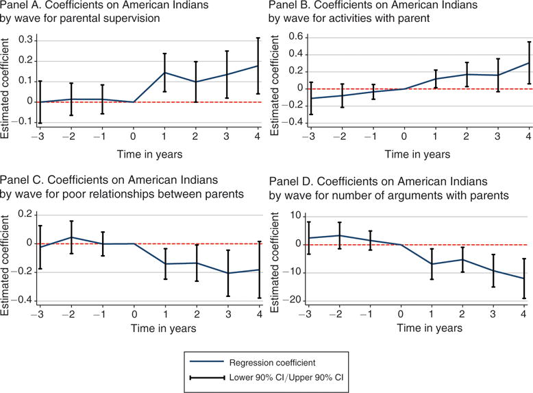
The Effects of Casino Transfers on Parental Behaviors around the Time of Casino Opening

In panel B, we show a similar analysis for the effect of the casino payments on whether the child reports enjoyable activities with the parent. Again, the answers are coded from 0 (not enjoyable) to 2 (most enjoyable). The children from households receiving the casino transfer payments report an increase in the probability of enjoyable activities with their mothers once the casino payments begin and this increase is statistically significant. Overall the effect of having additional household income is an improvement in parental supervision of their children and relationships with their children. Of note, these two outcomes are reported by separate respondents so that we can conclude that the estimated effects are not just a result of improved general outlook on life among parents receiving the transfers.²³

In panel C, we test whether the primary respondent parent reports a poor relationship with the other parent. This is a dummy variable, which takes the value 1 of the relationship between the parents in poor. In the figure, there is little systematic movement in the reporting of this variable by survey wave prior to the casino payments. However, the parents in households receiving the income transfers report a reduction in poor relationships (which indicates an improvement in parents’ relationships once the income transfers begin. Similarly, panel D shows the reporting of the number of arguments between parents and children by survey wave. This is a count variable of the number of arguments with children in the three months prior to the interview, as reported by the primary parent. After the casino payments begin we observe a reduction in the number of arguments between children and parents. Overall, we find convincing evidence that the casino transfers resulted in a large improvement in parents’ relationships with children and with their own spouses.

These findings offer strong evidence that there is a general improvement in the relationships within the household after the unconditional transfers begin. Two possible factors that could drive these results and also affect children’s outcomes may be changes in family composition brought about by divorce or (re) marriage and parental time use. We note that there is no change in parental marital status as a result of the unconditional cash transfers, as evidenced by the estimates reported in Appendix Table 8. Thus, we infer that these results are driven by changes within existing couples rather than endogenous (dissolution of) marriage in response to the transfers. In Appendix Table 9 we show that the results do not appear to be driven by changes in parental leisure or work activities, as we find no effects of the transfers on a variety of employment-related outcomes; additionally, the estimated coefficients themselves are quite small in magnitude and never achieve statistical significance at conventional levels.

Parental Mental Health Outcomes

The unconditional transfers may contribute to an improvement in a parent’s own mental health and a reduction in their own stress levels as found in other studies (Evans and Garthwaite 2014; Milligan and Stabile 2011; Jones, Milligan, and Stabile 2015). We are limited in our investigation of this potential channel by the availability of survey questions about the parents’ own health and stress levels. In Figure 4, we examine the evolution of parental mental health during the period of observation using an indicator of whether none, one, or both parents ever sought treatment by a mental health professional. The variable is reported by the respondent parent, typically the mother in the household, and ranges from 0 to 2. The results indicate that receiving casino payments reduces the likelihood that parents would seek treatment by a mental health professional; it is statistically significant at the 90 percent level 2, 3, and 4 years after the start of the casino transfers. We provide the regression results for the receipt of the casino transfer in Appendix Table 10.

Figure 4.

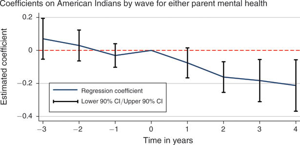
The Effects of Casino Transfers on Parental Mental Health around the Time of Casino Opening

Of course, the results here only indicate that after the casino payments, parents were less likely to report having to seek mental health treatment. This may mean that parents experienced less mental health problems or that they simply avoided treatment more systematically. It is not possible to distinguish between the two possibilities. Notably, similar evidence is presented by Cesarini et al. (2015), who use prescription data from Sweden and find reductions in the use of anti-anxiety and sleep-related medication by adults who won the lottery.

VI. Robustness Checks and Specification Checks

This section presents sensitivity and robustness checks, and it explores the possibility of heterogeneous effects across predetermined characteristics. Previous research suggests that there may be important differences in transfer effects by the households’ initial poverty status (Akee et al. 2010, 2013; Costello et al. 2003).²⁴ In Appendix Table 11 we provide the main analysis from Table 3 by initial household poverty status. The results indicate that the coefficients are of the expected signs for the first four columns in both panels and attain statistical significance in four out of the eight regressions. Overall, the coefficients show some slight differences, but the effects are not consistently different across initial poverty level.

In Appendix Table 12 we separate out the behavioral and emotional disorder reports contained in the survey by whether they are reported by the parent alone, child alone or both combined. In our main analysis we use the combined reports as is standard in the psychology literature. The analysis of the separate responses by parent and child suggests that the estimated reduction in emotional disorder symptoms is mostly driven by the child’s reporting. On the other hand, the reduction in behavioral disorders is driven primarily by the parent’s reporting of child behaviors. This is intuitively appealing because child behaviors are likely to be more accurately reported by the parent, while the child’s emotional state is probably better known to the child herself.

In Appendix Table 13 we explicitly test for differences in coefficients for children residing on or off the reservation and we fail to reject the hypothesis that they are equal in all cases except for neuroticism. The magnitudes and statistical significance for the other four outcome variables do not differ systematically in one direction or the other.

Finally, we examine whether there were other institutional or community-level programs (or funding) at this time period that coincide with the casino transfer payments. One potential source could be an increase in US federal funding for American Indians in the mid-1990s. Examining data from Walke (2000), we find that there has been a sharp reduction in federal funding for American Indians across the board since the 1980s and a slight drop in 1996 as well (see Appendix Figure 5). We also checked the US Senate Documents for the Bureau of Indian Affairs appropriations and found that there were no new funding allocations for the Eastern Band of Cherokee Indians during this time period.

Furthermore, there is little evidence to suggest that there were new EBCI tribal government health or educational programs developed in this relatively short time period. If new programs had been developed, then that might play a role in explaining the observed results for these cohorts of children. However, the evidence suggests that new programs and expanded tribal government spending (due to the casino revenues) occurred only in the early 2000s: after the youngest age cohort of children had already turned 16 and thus after our observation window (Johnson, Kasarda, and Appold 2011, Table 14).

VII. Discussion and Conclusions

Our main results indicate that an increase in unconditional household income reduces the prevalence of behavioral and emotional disorders and improves the personality traits of affected children. Given the panel nature of our data and the fact that we have survey waves extending into early adulthood, it is natural to ask whether the observed improvements in childhood personality traits and behaviors are associated with improvements in long-run outcomes. In Appendix Table B1, we identify the association between the levels of age 16 disorders and personality traits and full-time employment and educational attainment of non-Indians at age 25. The table shows that lower levels of behavioral or emotional disorders are both associated with higher levels of educational attainment and full-time employment for the non-Indian sample. We use this group to identify the association because it was not affected by the change in household income. Conversely, increased levels of the three personality traits are associated with higher levels in educational attainment and employment for this same group.

We next show the relationship for the American Indian children who were treated to the unconditional cash transfers. While we cannot identify the effects in a causal manner, we are able to identify simple associations. We assume that the relationship between the personality traits and behavioral disorders on long-run outcomes for non-Indians approximates the corresponding relationship for the American Indian population. In Appendix Table B2 we decompose the differences in educational attainment and employment probabilities at age 25 across the different age cohorts in our sample by using the coefficient from the non-Indian group. We find that the resulting change (due to the increased household income during adolescence) in conscientiousness is associated with an increase in education of 0.134 (or approximately 28 percent of the observed change) and full-time employment of 0.013 (or approximately 5.6 percent of the observed change). These results are suggestive of the potential long-run payoff to the increase in adolescent personality traits and behaviors.

Our research adds to the literature on the effect of unconditional cash transfers to families on child personality traits and behaviors in a quasi-experimental setting. To our knowledge, the research we describe is the first to examine this type of income intervention and its resulting effect on child personality traits and psychiatric disorders accounting for unobserved individual characteristics in a longitudinal setting. It is also the first to examine potential mechanisms using longitudinal data on parents of the population of interest. Our analysis focuses on a particular group, American Indians, that often goes understudied in standard datasets due to small population sizes. There is little research comparing behavioral responses among this group to other populations in the United States. Thus, additional research is warranted before extrapolating our results to other demographic groups. While we acknowledge the differences across this group and its comparison group of non-Hispanic white children, we have found that there are substantial similarities in average income, parental marital status, unemployment rates, and education levels for this group with our rural minority populations such as African Americans and other Native Americans.

The effects reported here are robust to including individual fixed effects and are not explained by changes in parental time use, employment, marital status, or other government programs. The size of the effects is relatively large; the unconditional cash transfer reduces behavioral disorder symptoms by 23 percent of a standard deviation and increases conscientiousness by 20 percent of a standard deviation. We have also shown that the effect is most significant for children who initially had the lowest endowments in these personality traits and those who exhibited more emotional or behavioral disorders. This suggests that parents (across households) may be reacting to the exogenous cash transfers by compensating for their children who have lower levels of mental health and poorer personality traits.

Given the longitudinal nature of our data, we are able to investigate several potential mechanisms responsible for the observed change in child outcomes. While there was little to no evidence for changes in parental employment (a proxy for time spent with children), there was significant evidence to suggest that parental relationships with children and with their spouses (partners) improved. Other researchers have shown conclusively that increased incomes have significantly improved parental outlook, mental health and happiness. Therefore, the results here provide additional evidence that while total parental time with the child may not have changed, a better quality of interactions by itself may have an important impact on child behavior and personality.

One important caveat regarding our research is worth repeating. The unconditional cash transfer analyzed here is unique because it is relatively large, does not come with any restrictions on use, and has been effectively perceived as a permanent income change for our study population. It is distinctly possible that any of these features or a combination of them contributed to the effect on the long-term outlook of the treated households and children. Additional research for the effect of shorter-term household income changes with a quasi-experimental design would help to establish the relevant threshold necessary to ascertain an effect on child behavior and personality traits.

Appendix A. Tables and Figures

Appendix Table 1.

Variables from GSMS Used to Create Big 5 Personality Traits: Agreeableness, Conscientiousness, and Neuroticism

	Emotional	Behavioral
Agreeableness
Number of arguments with Parent1a	Sep. distress from home or att. figure	Often bullies, threatens, or intimidates others
Number of arguments with other adultsa	Worry about possible harm	Often initiates physical fights
Number of arguments with peers at school	Worry about calamitous separation	Has used a weapon that can cause serious physical harm to others
Irritability intensitya,b	Persistent reluctance refusal / to go to school	Has been physically cruel to people
Bullies/extortiona	Avoidance of being alone	Has been physically cruel to animals
Cruelty to animalsa	Reluctance to sleep away	Has stolen while confronting a victim (e.g., mugging, purse snatching, extortion, armed robbery)
Rumors	Separation nightmares	Has forced someone into sexual activity
Spiteful or vindictivea	Physical symptoms	Has deliberately engaged in fire setting with the intention of causing serious damage
Loses tempera	Diagnosed panic attacks	Has deliberately destroyed others’ property (other than by fire setting)
Angry or resentfula	Meeting criteria for obsessive compulsive disorder	Has broken into someone else’s house, building, or car
	Social anxiety	Often lies to obtain goods or favors or to avoid obligations (i.e., “cons” others)
Conscientiousness	Fear public performance	Has stolen items of nontrivial value without confronting a victim
Lying intensitya	Social phobia, animal type	Often stays out at night despite parental prohibitions, beginning before age 13 years
Impulsive intensity	Social phobia, natural, other	Has run away from home overnight at least twice while living in parental or parental surrogate home
Rule-breaking intensity	Social phobia, blood, injection, injury	Is often truant from school, beginning before age 13 years
Concentration/difficulty paying attentiona,b	Agoraphobia	Often loses temper
	Post-traumatic stress painful recall screen positive	Often argues with adults
Neuroticism	Post-traumatic stress hyperarousal screen positive	Often actively defies or refuses to comply with adults’ requests or rules
Feels unloved	Post-traumatic stress avoidance screen positive	Often deliberately annoys people
Feeling of inferiority to others	Restlessness, keyed up, on edge	Often blames others for his or her mistakes or misbehavior
Subject feels sorry for himselfb	Easy fatigability	Is often touchy or easily annoyed by others
Feels helpless in general	Difficulty concentrating, mind blank	Is often angry and resentful
Depressed moodb	Irritability	Is often spiteful or vindictive
	Muscle soreness	Often fails to give close attention to details or makes careless mistakes
	Trouble falling or staying asleep	Often has difficulty sustaining attention in tasks or play activities
	Excessive worry (a symptoms of generalized anxiety disorder)	Often does not seem to listen when spoken to directly
	Frequent somatic complaints for which no physical basis could be found	Often does not follow through on instructions and fails to finish school work, chores
	Excessive need for reassurance	Often has difficulty organizing tasks and activities
	Marked feelings of tension or inability to relax	Often avoids, dislikes, or is reluctant to engage in tasks that require sustained mental effort
	Depressed/irritable mood	Often loses things necessary for tasks or activities
	Anhedonia or lose interest	Is often easily distracted by extraneous stimuli
	Weight loss or gain/dysthymia	Is often forgetful in daily activities
	Insomnia or hypersomnia	Often fidgets with hands or feet or squirms in seat
	Psychomotor agitation/retardation	Often leaves seat in classroom or in other situations in which remaining seated is expected
	Fatigue or loss of energy	Often runs about or climbs excessively in situations in which it is inappropriate
	Low self-esteem/worthlessness/guilt	Often has difficulty playing or engaging in leisure activities quietly
	Diff concentrating/thinking/deciding	Is often “on the go” or often acts as if “driven by a motor”
	Think about, plan, or attempt suicide	Often talks excessively
	Hopelessness	Often blurts out answers before questions have been completed
		Often has difficulty awaiting turn
		Often interrupts or intrudes on others (e.g., butts into conversations or games)

^aindicates overlap with behavioral

^bindicates overlap with emotional

Appendix Table 2.

Summary of Relevant Background Findings in the Previous Literature

Big 5 measure	Study	Education measure used in correlation	Correlation coefficient	Reporting source
Conscientiousness	Our study	Years of attained education	0.311 (0.105)	Parent report
	Pororat (2009)	Education grade: primary, secondary, or tertiary	0.283 (primary)	Meta analysis
			0.206 (secondary) 0.241 (tertiary)
	Denissen et al. (2008)	Education level (1-primary through 5-higher professional)	0.15	Self assessment
	Borghans et al. (2008)	Years of attained education	0.11	Meta analysis
	Goldberg et al. (1998)	Years of attained education	0.11	Self reported
Agreeableness	Our study	Years of attained education	0.181 (0.1)	Parent report
	Pororat (2009)	Education grade: primary, secondary, or tertiary	0.298 (primary)	Meta analysis
			0.051 (secondary) 0.06 (tertiary)
	Denissen et al. (2008)	Education level (1-primary through 5-higher professional)	0.05	Self assessment
	Borghans et al. (2008)	Years of attained education	−0.13	Meta analysis
	Goldberg et al. (1998)	Years of attained education	−0.12	Self reported
Neuroticism	Our study	Years of attained education	0.29 (0.111)	Parent report
“Emotional Stability”	Pororat (2009)	Education grade: primary, secondary, or tertiary	0.242 (primary)	Meta analysis
			0.014 (secondary) 0.0 (tertiary)
neuroticism	Denissen et al. (2008)	Education level (1-primary through 5-higher professional)	−0.15	Self assessment
“Emotional Stability”	Borghans et al. (2008)	Years of attained education	0.06	Meta analysis
“Emotional Stability”	Goldberg et al. (1998)	Years of attained education	0.06	Self reported

Appendix Table 3.

Comparison of Economic Characteristics with Other American Indian Tribes and Relevant Demographic Groups

	1990 Census report on American Indians	Social explorer	IPUMS 1990
	Eastern Cherokee (reservation)	All 11 counties	All Native Americans	Rural Native Americans	Rural African Americans	All of United States	Rural United States
Rural status	99%a	65%	54%	100%	100%	32%	100%
Median family income	$17,778	$27,275	$20,000	$18,000	$17,000	$32,030	$29,400
Family size	2.95		3.86	4.17	4.11	3.28	3.4
Own house	70%	75%	58%	68%	70%	69%	80%
Married	50%	60%	47%	49%	41%	58%	66%
Percent of age 25 + with a high school degree	70%	69%	69%	64%	53%	79%	75%
Unemployment rate	12%a	6%	15%	18%	12%	6%	6%
Per capita income	$6,543	$11,691	$11,362	$9,905	$9,165	$17,922	$15,677

Source: 1990 Census Report on American Indians; Social Explorer, 1990 County Data; IPUMS 1990, 1% Sample

^aTaylor and Akee (2014)

Appendix Table 4.

Mean Differences by Age Cohort and American Indian Parent Status at Survey Wave 1

Non American Indian cohorts
Differences between cohort 1 and cohort 2
	Cohort 1 mean	Cohort 2 mean	Difference	SE of difference
Number of American Indian parents	N / A	N / A
American Indian	0.019	0.036	−0.017	0.012
Male child indicator	0.562	0.596	− 0.034	0.037
Mother has a high school degree/GED	0.297	0.270	0.027	0.033
Father has a high school degree/GED	0.184	0.184	0.000	0.029
Mother has more than a high school degree	0.462	0.518	−0.056	0.037
Father has more than a high school degree	0.281	0.309	− 0.028	0.034
Initial household income	29,367.98	32,652.17	− 3,284.19	1,331.824
Differences between cohort 2 and cohort 3
	Cohort 2 mean	Cohort 3 mean	Difference	SE of difference
Number of American Indian parents	N / A	N /A
American Indian indicator	0.036	0.071	−0.034	0.017
Male child indicator	0.596	0.526	0.070	0.038
Mother has a high school degree/GED	0.270	0.279	−0.009	0.035
Father has a high school degree/GED	0.184	0.141	0.043	0.029
Mother has more than a high school degree	0.518	0.471	0.047	0.039
Father has more than a high school degree	0.309	0.292	0.018	0.036
Initial household income	32,652.17	32,154.88	497.290	1,399.523
Differences between cohort 1 and cohort 3
	Cohort 1 mean	Cohort 3 mean	Difference	SE of difference
Number of American Indian parents	N/A	N/A
American Indian indicator	0.019	0.071	−0.052	0.015
Male child indicator	0.562	0.526	0.037	0.038
Mother has a high school degree/GED	0.297	0.279	0.018	0.035
Father has a high school degree/GED	0.184	0.141	0.043	0.028
Mother has more than a high school degree	0.462	0.471	−0.009	0.038
Father has more than a high school degree	0.281	0.292	−0.011	0.035
Initial household income	29,367.90	32,154.88	− 2,786.9	1,364.668
American Indian cohorts
Differences between cohort 1 and cohort 2
	Cohort 1 mean	Cohort 2 mean	Difference	SE of difference
Number of American Indian parents	1.355	1.387	−0.032	0.066
American Indian indicator	0.927	0.981	− 0.054	0.028
Male child indicator	0.509	0.547	− 0.038	0.068
Mother has a high school degree/GED	0.400	0.330	0.070	0.066
Father has a high school degree/GED	0.218	0.160	0.058	0.053
Mother has more than a high school degree	0.373	0.415	−0.042	0.067
Father has more than a high school degree	0.218	0.236	− 0.018	0.057
Initial household income	21,952.38	21,212.12	740.260	2,179.163
Differences between cohort 2 and cohort 3
	Cohort 2 mean	Cohort 3 mean	Difference	SE of difference
Number of American Indian parents	1.387	1.296	0.090	0.070
American Indian indicator	0.981	0.926	0.055	0.030
Male child indicator	0.547	0.543	0.004	0.074
Mother has a high school degree/GED	0.330	0.333	−0.003	0.070
Father has a high school degree/GED	0.160	0.259	− 0.099	0.059
Mother has more than a high school degree	0.415	0.383	0.032	0.073
Father has more than a high school degree	0.236	0.198	0.038	0.061
Initial household income	21,212.12	25,000.00	−3,787.88	2,373.339
Differences between cohort 1 and cohort 3
	Cohort 1 mean	Cohort 3 mean	Difference	SE of difference
Number of American Indian parents	1.355	1.296	0.058	0.069
American Indian indicator	0.927	0.926	0.001	0.038
Male child indicator	0.509	0.543	−0.034	0.073
Mother has a high school degree/GED	0.400	0.333	0.067	0.071
Father has a high school degree/GED	0.218	0.259	−0.041	0.062
Mother has more than a high school degree	0.373	0.383	− 0.010	0.071
Father has more than a high school degree	0.218	0.198	0.021	0.060
Initial household income	21,952.38	25,000.00	−3,047.62	2,366.745

Appendix Table 5.

The Effect of Casino Transfers on Children’s Emotional and Behavioral Disorder Symptoms and Personality Traits

	Behavioral disorder symptoms (1)	Emotional disorder symptoms (2)	Conscientiousness (3)	Agreeableness (4)	Neuroticism (5)
SurveyWave 1 × YoungestCohorts × AI	−0.0705 (0.148)	−0.168 (0.170)	0.157 (0.185)	0.119 (0.222)	0.104 (0.254)
SurveyWave 2 × YoungestCohorts × AI	0.0369 (0.113)	0.0138 (0.136)	−0.0651 (0.143)	−0.0134 (0.167)	−0.236 (0.185)
SurveyWave 3 × YoungestCohorts × AI	−0.0316 (0.0863)	−0.0738 (0.0903)	−0.150 (0.111)	0.199 (0.129)	−0.0912 (0.125)
SurveyWave 4 × YoungestCohorts × AI	Omitted category	Omitted category	Omitted category	Omitted category	Omitted category
SurveyWave 5 × YoungestCohorts × AI	−0.144 (0.126)	−0.241 (0.114)	−0.0278 (0.177)	0.187 (0.220)	0.137 (0.151)
SurveyWave 6 × YoungestCohorts × AI	−0.257 (0.143)	−0.392 (0.137)	0.210 (0.168)	0.608 (0.178)	0.338 (0.206)
SurveyWave 7 × YoungestCohorts × AI	−0.408 (0.169)	−0.568 (0.189)	0.286 (0.210)	0.749 (0.242)	0.754 (0.265)
SurveyWave 8 × YoungestCohorts × AI	−0.501 (0.203)	−0.655 (0.238)	0.292 (0.241)	0.993 (0.276)	1.097 (0.318)
Individual fixed effects?	N	N	N	N	N
Mean of dependent variable	0	0	0	0	0
Observations	6,674	6,674	6,309	6,084	6,298
Adjusted R2	0.026	0.028	0.050	0.070	0.049
Number of individuals	1,420	1,420	1,420	1,420	1,420

Notes: Survey wave interaction variables are the interaction of American Indian × YoungestCohorts with each wave dummy variable. The fourth survey wave interaction is omitted. Casino payments began after wave 4 for only American Indian children. All regressions include secondary interaction variables American Indian × Cohort and Cohort × Survey Wave (indicators), and dummies for survey wave, American Indian, and cohort. They also include the number of children younger than 6 living in the household, age of the child and its interaction with American Indian, year and month of interview controls, and a constant term. Standard errors clustered at the individual level.

Appendix Table 6.

Heterogeneous Effect of Casino Transfers by Standardized Initial Conditions

	Behavioral disorder symptoms (1)	Emotional disorder symptoms (2)	Conscientiousness (3)	Agreeableness (4)	Neuroticism (5)
Receipt of cash transfer	−0.0560 (0.0813)	−0.0712 (0.114)	0.0403 (0.119)	0.115 (0.130)	0.215 (0.134)
Interaction of pre-casino behavioral disorder symptoms ever above median × receipt of cash transfer	−0.163 (0.0705)
Interaction of pre-casino emotional disorder symptoms ever above median × receipt of cash transfer		−0.257 (0.0796)
Interaction of pre-casino conscientiousness ever below median × receipt of cash transfer			0.328 (0.104)
Interaction of pre-casino agreeableness ever below median × receipt of cash transfer				0.334 (0.123)
Interaction of pre-casino neuroticism ever below median × receipt of cash transfer					0.417 (0.215)
Individual fixed effects	Y	Y	Y	Y	Y
Mean of dependent variable	0.000	0.000	0.000	0.000	0.000
Observations	6,674	6,674	6,309	6,084	6,298
R2	0.031	0.025	0.047	0.076	0.049
Number of individuals	1,420	1,420	1,414	1,404	1,413

Notes: Receipt of cash transfer is the triple difference coefficient from our empirical specification in equation (1). It is an interaction of American Indian × YoungestCohorts × After Casino. Casino payments began after wave 4 for only American Indian children. Interaction variables are constructed by interacting the Receipt of Cash Transfer with an indicator for the initial endowment of the outcome variable (ever above median for each respective measure in the first three survey waves). All regressions include secondary interaction variables American Indian × Cohort and Cohort × SurveyWave (indicators), and dummies for survey wave, American Indian, and cohort. They also include the number of children younger than six living in the household, child’s age and its interaction with American Indian, year and month of interview controls, and a constant term. Individual fixed effects are included in all specifications. Standard errors clustered at the individual level.

Appendix Table 7.

Effects of Casino Payments on Parental Behaviors and Relationships

	Adequate parental supervision (1)	Enjoyable relationship with parent (2)	Poor relationship between parents (3)	Arguments with parent (4)
Panel A
Receipt of cash transfer	0.118 (0.0440)	0.109 (0.0499)	−0.160 (0.0548)	−6.245 (2.397)
Individual fixed effect	N	N	N	N
Mean of dependent variable	1.942	1.885	0.319	5.635
Observations	5,334	5,906	6,101	6,477
R2	0.018	0.018	0.024	0.014
Panel B
Receipt of cash transfer	0.0954 (0.0453)	0.0952 (0.0506)	−0.148 (0.0544)	−5.287 (2.318)
Individual fixed effect	Y	Y	Y	Y
Mean of dependent variable	1.942	1.885	0.319	5.635
Observations	5,334	5,906	6,101	6,477
R2	0.015	0.011	0.036	0.011
Number of individuals	1,279	1,343	1,407	1,417
Panel C
SurveyWave 1 × YoungestCohorts × AI	<0.0001 (0.0626)	−0.110 (0.114)	−0.0241 (0.0914)	2.424 (3.487)
SurveyWave 2 × YoungestCohorts × AI	0.0141 (0.0478)	−0.0785 (0.0830)	0.0451 (0.0690)	3.302 (2.858)
SurveyWave 3 × YoungestCohorts × AI	0.0137 (0.0431)	−0.0335 (0.0526)	−0.00121 (0.0504)	1.536 (2.063)
SurveyWave 4 × YoungestCohorts × AI	Omitted category	Omitted category	Omitted category	Omitted category
SurveyWave 5 × YoungestCohorts × AI	0.145 (0.0568)	0.118 (0.0629)	−0.141 (0.0646)	−6.860 (3.300)
SurveyWave 6 × YoungestCohorts × AI	0.0990 (0.0603)	0.169 (0.0859)	−0.135 (0.0768)	−5.285 (2.679)
SurveyWave 7 × YoungestCohorts × AI	0.135 (0.0700)	0.161 (0.117)	−0.206 (0.0977)	−9.224 (3.510)
SurveyWave 8 × YoungestCohorts × AI	0.178 (0.0832)	0.306 (0.149)	−0.181 (0.120)	−12.00 (4.290)
Individual fixed effect	N	N	N	N
Mean of dependent variable	1.942	1.885	0.319	5.635
Observations	5,334	5,906	6,101	6,477
R2	0.018	0.019	0.024	0.014

Notes: Receipt of cash transfer is the interaction of American Indian × YoungestCohorts × After Casino. Casino payments began after wave 4 for only American Indian children. All regressions include secondary interaction variables American Indian × Cohort and Cohort × SurveyWave (indicators), and dummies for survey wave, American Indian, and cohort. They also include the number of children younger than six in the household, child’s age and its interaction with American Indian, year and month of interview controls, and a constant term. All specification in panel B include also an individual fixed effect. Panel C includes all of the controls in panel A and the survey wave interactions are an interaction of American Indian × YoungestCohorts with indicator variables for each of the eight survey waves (survey wave 4 omitted). Standard errors clustered at the individual level.

Appendix Table 8.

Effects of Casino Transfers on Parental Marital Status

	Parents currently married (1)	Parents currently married (2)
Receipt of cash transfer	−0.0336 (0.0261)	−0.00262 (0.0362)
Individual fixed effects	Y	N
Mean of dependent variable	0.457	0.457
Observations	6,443	6,443
R2	0.050	0.046
Number of individuals	1,417	1,417

Notes: Receipt of cash transfer is the triple difference coefficient from our empirical specification in equation (1). It is an interaction of American Indian × YoungestCohorts × After Casino. Casino payments began after wave 4 for only American Indian children. All regressions include secondary interaction variables American Indian × Cohort and Cohort × SurveyWave (indicators), and dummies for survey wave, American Indian, and cohort. They also include the number of children younger than six living in the household, child’s age and the interaction of age with American Indian, year and month of interview controls, and a constant term. Column 1 includes also an individual fixed effect. Standard errors clustered at the individual level.

Appendix Table 9.

Casino Transfers and Parental Employment

Variables	Labor force participation			Full-time			Full- or part-time
	Mother in labor force (1)	Father in labor force (2)	Either in labor force (3)	Mother full-time employed (4)	Father full-time employed (5)	Either parent full-time employed (6)	Mother part-time employed (7)	Father part-time employed (8)	Either parent part-time employed (9)
Panel A
Receipt of cash transfer	0.00405 (0.0489)	0.0223 (0.0332)	−0.0123 (0.0384)	0.00405 (0.0489)	0.0159 (0.0577)	−0.0123 (0.0424)	0.0175 (0.0487)	−0.00841 (0.0464)	0.0113 (0.0419)
Mean of dependent variable	0.625	0.942	0.823	0.625	0.878	0.804	0.761	0.904	0.861
Observations	5,316	3,282	5,746	5,316	3,282	5,746	5,316	3,282	5,746
R2	0.026	0.022	0.027	0.026	0.032	0.031	0.030	0.040	0.032
	On reservation only
	Labor force participation			Full-time			Full- or part-time
Panel B
Receipt of cash transfer	0.157 (0.189)	0.127 (0.300)	0.0932 (0.179)	0.157 (0.189)	0.0303 (0.275)	0.0783 (0.179)	0.119 (0.244)	0.168 (0.308)	0.167 (0.189)
Mean of dependent variable	0.642	0.922	0.782	0.642	0.787	0.747	0.734	0.819	0.807
Observations	943	475	1,000	943	475	1,000	943	475	1,000
R2	0.085	0.056	0.064	0.085	0.067	0.068	0.093	0.069	0.073

Notes: Receipt of cash transfer is the triple difference coefficient from our empirical specification in equation (1). It is an interaction of American Indian × YoungestCohorts × After Casino. Casino payments began after wave 4 for only American Indian children. All regressions include secondary interaction variables American Indian × Cohort and Cohort × SurveyWave (indicators), and dummies for survey wave, American Indian, and cohort. They also include the number of children younger than six living in the household, child’s age and the interaction of age with American Indian, year and month of interview controls, and a constant term. Standard errors clustered at the individual level.

Appendix Table 10.

Parental Mental Health and Casino Payments

	Ever treated by mental health professional, either parent
	(1)	(2)	(3)
Panel A
Receipt of cash transfer	−0.0761 (0.0458)	−0.0559 (0.0460)
SurveyWave 1 × YoungestCohorts × AI			0.0705 (0.0750)
SurveyWave 2 × YoungestCohorts × AI			0.0298 (0.0569)
SurveyWave 3 × YoungestCohorts × AI			−0.0309 (0.0433)
SurveyWave 4 × YoungestCohorts × AI			Omitted category
SurveyWave 5 × YoungestCohorts × AI			−0.0755 (0.0553)
SurveyWave 6 × YoungestCohorts × AI			−0.162 (0.0565)
SurveyWave 7 × YoungestCohorts × AI			−0.183 (0.0775)
SurveyWave 8 × YoungestCohorts × AI			−0.213 (0.0948)
Individual fixed effect?	N	Y	N
Mean of dependent variable	0.219	0.219	0.219
Observations	6,471	6,471	6,471
R2	0.046	0.065	0.047
Number of individuals	1,417	1,417	1,417

Notes: Receipt of cash transfer is the triple difference coefficient from our empirical specification in equation (1). It is an interaction of American Indian × YoungestCohorts × After Casino. Casino payments began after wave 4 for only American Indian children. All regressions include secondary interaction variables American Indian × Cohort and Cohort × SurveyWave (indicators), and dummies for survey wave, American Indian, and cohort. They also include the number of children younger than six in the household, child’s age, and the interaction of age with American Indian, year and month of interview controls, and a constant term. Column 2 includes an individual fixed effect. Column 3 includes all of the controls in panel A. Standard errors clustered at the individual level.

Appendix Table 11.

Transfer Effects by Initial Household Poverty Status

	Behavioral disorder symptoms (1)	Emotional disorder symptoms (2)	Conscientiousness (3)	Agreeableness (4)	Neuroticism (5)
Panel A. Not in poverty
Receipt of cash transfer	−0.312 (0.129)	−0.218 (0.132)	0.276 (0.176)	0.355 (0.204)	0.164 (0.197)
Initially in poverty	N	N	N	N	N
Mean of dependent variable	−0.0522	−0.0307	0.0733	0.0200	0.0330
Observations	3,836	3,836	3,669	3,564	3,661
R2	0.032	0.033	0.052	0.077	0.052
Panel B. Initially in poverty
Receipt of cash transfer	−0.171 (0.159)	−0.498 (0.155)	0.201 (0.193)	0.403 (0.222)	0.495 (0.208)
Initially in poverty	Y	Y	Y	Y	Y
Mean of dependent variable	0.0706	0.0415	−0.102	−0.0283	−0.0458
Observations	2,838	2,838	2,640	2,520	2,637
R2	0.040	0.036	0.067	0.077	0.052

Notes: Receipt of cash transfer is the triple difference coefficient from our empirical specification in equation (1). It is an interaction of American Indian × YoungestCohorts × After Casino. Casino payments began after wave 4 for only American Indian children. All regressions include secondary interaction variables American Indian × Cohort and Cohort × SurveyWave (indicators), and dummies for survey wave, American Indian, and cohort. They also include the number of children younger than six in the household, child’s age and the interaction with American Indian, year and month of interview controls, and a constant term. Standard errors clustered at the individual level.

Appendix Table 12.

Effects on Behavior and Emotional Disorders by Source of Reporting

	Behavioral disorder symptoms: both reports (1)	Emotional disorder symptoms: both reports (2)	Behavioral disorder symptoms: parent report alone (3)	Emotional disorder symptoms: parent report alone (4)	Behavioral disorder symptoms: child report alone (5)	Emotional disorder symptoms: child report alone (6)
Receipt of cash transfer	−0.233 (0.104)	−0.374 (0.104)	−0.234 (0.106)	−0.260 (0.105)	−0.160 (0.112)	−0.337 (0.105)
Mean of dependent variable	0	0	0	0	0	0
Observations	6,674	6,674	6,499	6,674	6,410	6,674
R2	0.025	0.027	0.023	0.023	0.033	0.021

Notes: Receipt of cash transfer is the triple difference coefficient from our empirical specification in equation (1). It is an interaction of American Indian × YoungestCohorts × After Casino. Casino payments began after wave 4 for only American Indian children. All regressions include secondary interaction variables American Indian × Cohort and Cohort × SurveyWave (indicators), and dummies for survey wave, American Indian, and cohort. They also include the number of children younger than six in the household, child’s age and the interaction with American Indian, year and month of interview controls, and a constant term. Standard errors clustered at the individual level.

Appendix Table 13.

Main Regression Results Separated by On or Off Reservation Status

	Behavioral disorder symptoms		Emotional disorder symptoms		Conscientiousness		Agreeableness		Neuroticism
	(1)	(2)	(3)	(4)	(5)	(6)	(7)	(8)	(9)	(10)
Receipt of cash transfer	−0.381 (0.397)	−0.203 (0.106)	−0.199 (0.268)	−0.328 (0.182)	0.753 (0.444)	0.282 (0.187)	0.337 (0.511)	0.321 (0.227)	−0.289 (0.288)	0.356 (0.189)
On reservation	Y	N	Y	N	Y	N	Y	N	Y	N
p-value for equality of coefficients	0.6595		0.6867		0.3201		0.9775		0.0581
Observations	1,212	4,960	1,212	4,960	1,151	4,701	1,118	4,533	1,146	4,694
R2	0.058	0.025	0.046	0.030	0.072	0.052	0.051	0.067	0.031	0.051

Notes: Receipt of cash transfer is the triple difference coefficient from our empirical specification in equation (1). It is an interaction of American Indian × YoungestCohorts × After Casino. Casino payments began after wave 4 for only American Indian children. All regressions include secondary interaction variables American Indian × Cohort and Cohort × SurveyWave (indicators), and dummies for survey wave, American Indian, and cohort. They also include the number of children younger than six in the household, child’s age and the interaction with American Indian, year and month of interview controls, and a constant term. Standard errors clustered at the individual level.

Appendix Figure 1. Great Smoky Mountain Study of Youth Survey Schedule by Age Cohort and Year.

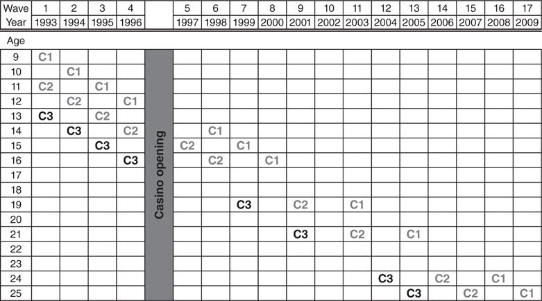
Notes: C1 represents the youngest age cohort (children initially nine years old at intake) for both American Indians and non-Indians. C2 represents the middle age cohort (children initially 11 years old at intake) and C3 represents the oldest age cohort (children initially 13 years old at intake). All cohorts were surveyed up to and including age 16 at an annual basis, then at ages 19, 21, 24, and 25. Casino operations on the Eastern Band of Cherokee Indians reservation in 1996.

Appendix Figure 2.

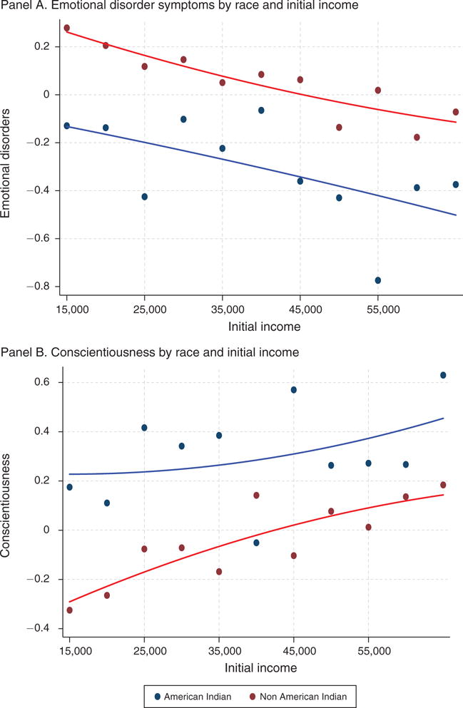
Relationship between Initial Income and Psychological Traits

Appendix Figure 3. American Indians and Non-Indians Combined (Triple Difference Coefficients) in First Three Survey Waves: All Three Cohorts.

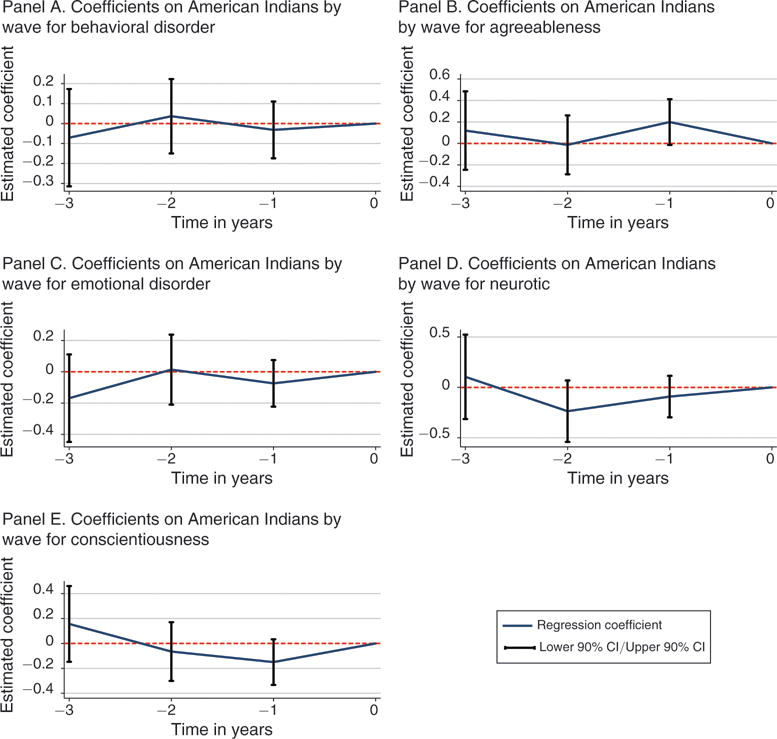
Notes: These five figures display the estimated coefficient from a triple interaction of American Indian × YoungestCohorts × SurveyWave. Year of Casino opening is the omitted category. These figures indicate that prior to the tribal cash payments there were no statistically significant differences in the trends of the outcome variables.

Appendix Figure 4.

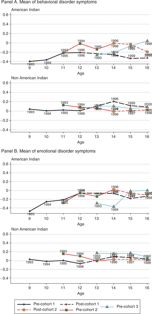
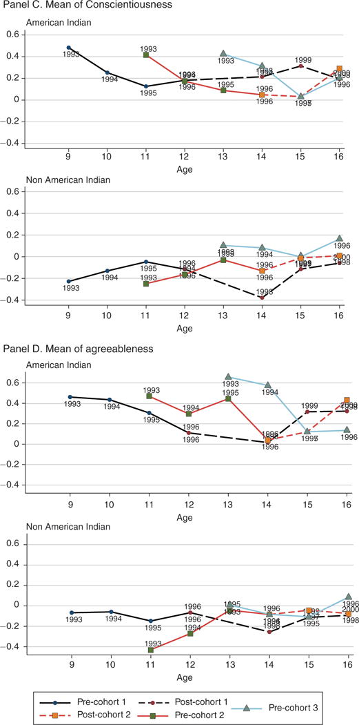
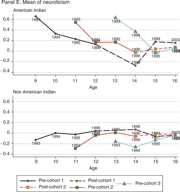
Mean of Dependent Variables by Survey Wave for All Three Cohorts Separated by American Indian Status

Appendix Figure 5. Bureau of Indian Affairs Expenditures Per Capita of the AI Population.

Source: Walke (2000)

Appendix B. Discussion of Long-Run Outcomes

Given the longitudinal nature of our data, we can examine the association between improved personality traits and reduction in emotional and behavioral disorders and adult outcomes. In Appendix Table B1, we identify the association between the levels of age 16 disorders and personality traits and age 25 outcomes such as employment and educational attainment of non-Indians. The non-Indians were not affected by changes in household income and thus did not have a change in disorders or personality traits during adolescence attributable to the same treatment. We find that measures of emotional and behavioral well-being at age 16 are positively related to labor market outcomes measured at age 25. Higher levels of behavioral and emotional disorders are associated with lower levels of educational attainment and employment probabilities. Conversely, higher levels of the three personality traits (conscientiousness, agreeableness, and neuroticism) at age 16 are associated with higher levels of these same outcomes measured at age 25.

We decompose the changes in age 25 educational attainment and full-time employment due to the associated changes in observed increases (by age 16) in conscientiousness and decreases in emotional disorders in the following table. We use the actual changes in child personality traits and emotional well-being at age 16 and the respective correlation coefficients from Table 9 to account for the observed increase in overall educational attainment and employment probability at age 25.

In Appendix Table B2, we present some results for the change in conscientiousness and emotional disorders (we do not present the other measures as they are highly correlated with one another and provide similar results). The total change in educational attainment and full-time employment (differencing across age cohorts and American Indian status) is given in the first row of the table as almost one-half a year of education (0.487 for education) and an increase of 22 percent in full-time employment (0.224 for full-time probability). We compute these measures using a simple difference-in-differences equation with no covariates for the age 25 outcome variables: educational attainment and full-time employment probability. The equation is the following:

$$\mathit{\text{EducationChange}}=({\mathit{\text{Education}}}_{Y,\mathrm{AI}}-{\mathit{\text{Education}}}_{O,\mathrm{AI}})-({\mathit{\text{Education}}}_{Y,\mathit{NonAI}}-{\mathit{\text{Education}}}_{O,\mathit{NonAI}}).$$

In the equation, the subscripts Y and O indicate youngest and oldest age cohorts respectively and AI and NonAI represent American Indian and non-Indian respectively. The four different variables labeled “Education” are the average educational attainment at age 25 for each of the four subgroups. A similar calculation is conducted for full-time employment probabilities at age 25.

In panel A, we provide the change in conscientiousness for the youngest age cohort of American Indians in our data (the second row). The coefficient on the third line comes from Appendix Table B1 and the fourth line provides the product of the value in row 2 and 3. We call this the total change in the fourth row. Finally, in the fifth row of Panel A we show the percent of the net change this total change represents, which is calculated as the ratio of row 4 to row 1. The change in conscientiousness is associated with approximately 28 percent of the difference in educational attainment for this age cohort and about 6 percent of the difference of full-time employment. Panel B provides a similar calculation for the reduction in emotional disorders and it is associated with approximately 21 percent of the change in educational attainment and about 5 percent of the change in full-time employment probability.

It is important to note that these measures are not independent (conscientiousness and emotional disorders) of one another; these results should not be interpreted as additive here. Additionally, it is not possible to fully provide a causal story for these long run (measured at age 25) outcomes and we stress that the results are meant to illustrate potential long-run effects.

Appendix Table B1.

Association between Long Run Outcomes (Age 25) for non American Indians using Age 16 Levels of Disorders and Personality Traits

	Years of educational attainment (1)	Full time employed (2)
Panel A. Behavioral disorder symptoms at age 16	−0.475 (0.0815)	−0.0734 (0.0165)
Panel B. Emotional disorder symptoms at age 16	−0.421 (0.114)	−0.0421 (0.0189)
Panel C. Conscientiousness score at age 16	0.517 (0.0876)	0.0481 (0.0169)
Panel D. Agreeableness score at age 16	0.263 (0.0753)	0.0412 (0.0147)
Panel E. Neuroticism score at age 16	0.279 (0.0683)	0.0504 (0.0112)

Notes: Pairs of coefficients are from separate regressions in each column. All regressions include Number of children less than 6, age fixed effects, wave fixed effects, age by race fixed effects and individual fixed effects and a constant. Standard errors clustered at the individual level.

Appendix Table B2.

Explaining Raw Differences in Outcomes by Changes in Age 16 Characteristics

	Education	Full-time
Net change (across cohort and AI status) at age 25	0.487	0.224
Panel A
Change in conscientiousness for age cohort 1 (age 16 - age 12)	0.260	0.260
Coefficient on conscientiousness from non AI	0.517	0.048
Total effect of change:	0.134	0.013
Percent of observed difference explained by increase in conscientiousness	0.276	0.056
Panel B
Change in emotional for age cohort 1 (age 16 - age 12)	−0.238	−0.238
Coefficient on emotional from non AI	−0.421	−0.042
Total effect of change:	0.100	0.010
Percent of observed difference explained by reduction in emotional	0.206	0.045

Appendix C. Robustness of Standard Errors

In the main analysis we cluster the standard errors on the individual child level. This section presents our main results with several alternative ways of clustering of the standard errors as well as permutation-based p-values as an alternative to the analytical (cluster-based) p-values. These p-values are based on permutation tests (Fisher 1935; Good 2005; Dinardo and Lee 2011) in which we randomly assign treatment status to subgroups of the study population. These tests do not depend on distributional assumptions and in small samples are likely to yield more reliable p-values for differences between treatments and controls. The permutation-based test assumes exchangeability of treatments and controls under the null. In order to conduct the test, we assign treatment status to subgroups of the study population based on county of residence (11 in total) American Indian race, cohort, and pre- or post-casino treatment period. For example, one of the possible permutation subgroup would be non-Indian children from the middle cohort residing in Cherokee county in the period after the casino opens. We then rerun the estimation using these subgroups as the treated population. The p-value corresponds to the percentile of the distribution where the observed true difference falls, relative to the other permutations.

Appendix Table C1.

The Effect of Casino Transfers on Children’s Emotional and Behavioral Disorder Symptoms and Personality Traits by Various Clustering Methods

		Behavioral disorder symptoms (1)	Emotional disorder symptoms (2)	Conscientiousness (3)	Agreeableness (4)	Neuroticism (5)
Panel A
Receipt of cash transfer		−0.233	−0.374	0.254	0.374	0.381
Standard errors clustered at:	Individual child	(0.104)	(0.104)	(0.128)	(0.147)	(0.141)
	Tract	(0.0888)	(0.0834)	(0.129)	(0.177)	(0.109)
	Counties	(0.0883)	(0.116)	(0.143)	(0.158)	(0.111)
	County by race by age group	(0.0950)	(0.0984)	(0.107)	(0.100)	(0.128)
p (analytical)		[0.025]	[<0.001]	[0.046]	[0.01]	[0.007]
p (resampling)		[0.007]	[0.007]	[0.013]	[<0.001]	[<0.001]
Individual fixed effects		N	N	N	N	N
Mean of dep. variable		0	0	0	0	0
SD of dep. variable		1	1	1.221	1.390	1.454
Observations		6,674	6,674	6,309	6,084	6,298
R2		0.025	0.027	0.049	0.068	0.046
Panel B
Receipt of cash transfer		−0.183	−0.306	0.200	0.292	0.311
Standard errors clustered at:	Individual child	(0.0910)	(0.102)	(0.121)	(0.146)	(0.137)
	Tract	(0.0774)	(0.0858)	(0.137)	(0.143)	(0.115)
	Counties	(0.0839)	(0.121)	(0.161)	(0.153)	(0.120)
	County by race by age group	(0.0762)	(0.106)	(0.117)	(0.0928)	(0.142)
p (analytical)		[0.075]	[0.008]	[0.145]	[0.080]	[0.046]
p (resampling)		[0.007]	[0.007]	[<0.001]	[<0.001]	[<0.001]
Individual fixed effects		Y	Y	Y	Y	Y
Mean of dep. variable		0	0	0	0	0
SD of dep. variable		1	1	1.221	1.390	1.454
Observations		6,674	6,674	6,309	6,084	6,298
R2		0.030	0.025	0.045	0.075	0.048
Number of individuals		1,420	1,420	1,414	1,404	1,413

Notes: For panels A and B, Receipt of cash transfer is the triple difference coefficient from our empirical specification. Casino payments began after wave 4 for only American Indian children. All regressions include secondary interaction variables and the main variables as specified in equation (1) They also include controls for age, age interacted with AI race, the number of children younger than six, year and month of interview controls, and a constant term. Panel B also includes an individual fixed effect. Standard errors clustered at the individual level, census tract, county, and a county by race by age group level.

Appendix D. Discussion of Factor Analysis for Construction of Personality Trait Indices

In order to create our personality trait indices, we identified questions from the GSMS survey that align most closely with the definitions for the Big 5 Personality Traits. We then used principal component analysis (a method of multidimensional scaling) to identify a weighting criteria for combining these variables into a single index for each personality trait. This process computes the eigenvectors and eigenvalues from these survey questions. Then, the weights are used to reduce the number of dimensions (variables) to a single one (our personality trait index). Eigenvectors are to weight the contribution of each variable to the new (single dimensional) index; variables which contribute most are weighted more heavily in this index. The variables used are listed in Appendix Table D1 for each of our personality trait indices for conscientiousness, agreeableness, and neuroticism. We do not have relevant measures for openness and extroversion in the GSMS questions and we do not attempt to create an indexed measure for those two personality traits. In the table we present the eigenvectors for each of our three personality indices.

There are, of course, many different ways indices could be created. A simple weighted average of the variables would be possible; however, this method is more appealing as it retains the orthogonal contributions of each variable to the new indices.

Our interest in showing the personality trait indices (in addition to the more clinical behavioral and emotional disorder symptoms) is that these measures are more common in the social science literature. We selected GSMS survey questions that were similar to those in the Behavioral Problem Index used in the NLSY data as well as the Big 5 Personality Traits scales questions.

Appdendix Table D1.

Eigenvectors for Each of the Principal Component Analysis for Personality Trait Indices

Conscientiousness	Eigenvector	Agreeableness	Eigenvector	Neuroticism	Eigenvector
Lying intensity	0.5805	Number of arguments with parent	0.399	Feels unloved	0.4433
Impulsive intensity	0.5473	Number of arguments with other adults	0.1704	Feeling of inferiority to others	0.4609
Rule breaking intensity	0.5897	Number of arguments with peers at school	0.2546	Subject feels sorry for himself	0.4943
Concentration/difficulty paying attention	0.1255	Irritability intensity	0.3625	Feels helpless in general	0.4313
		Bullies/extortion	0.2813	Depressed mood	0.4009
		Cruelty to animals	0.085
		Rumors	0.0912
		Spiteful or vindictive	0.4084
		Loses temper	0.3592
		Angry or resentful	0.4744

References

- Aizer Anna, Eli Shari, Ferrie Joseph, Lleras-Muney Adriana. The Long Term Impact of Cash Transfers to Poor Families. American Economic Review. 2016;106(4):935–71. doi: 10.1257/aer.20140529. [DOI] [PMC free article] [PubMed] [Google Scholar]
- Akee Randall, Copeland William, Costello E Jane, Simeonova Emilia. How Does Household Income Affect Child Personality Traits and Behaviors?: Dataset. American Economic Review. 2018 doi: 10.1257/aer.20160133. https://doi.org/10.1257/aer.20160133. [DOI] [PMC free article] [PubMed]
- Akee Randall KQ, Copeland William E, Keeler Gordon, Angold Adrian, Costello E Jane. Parents’ Incomes and Children’s Outcomes: A Quasi-Experiment Using Transfer Payments from Casino Profits. American Economics Journal: Applied Economics. 2010;2(1):86–115. doi: 10.1257/app.2.1.86. [DOI] [PMC free article] [PubMed] [Google Scholar]
- Akee Randall KQ, Simeonova Emilia, Copeland William, Angold Adrian, Costello E Jane. Young Adult Obesity and Household Income: Effects of Unconditional Cash Transfers. American Economics Journal: Applied Economics. 2013;5(2):1–28. doi: 10.1257/app.5.2.1. [DOI] [PMC free article] [PubMed] [Google Scholar]
- Akee Randall KQ, Taylor Jonathan B. Social and Economic Change on American Indian Reservations: A Databook of the US Censuses and American Community Survey, 1990–2010. Sarasota, FL: Taylor Policy Group, Inc.; 2014. [Google Scholar]
- Almlund Mathilde, Duckworth Angela Lee, Heckman James J, Kautz Tim D. Personality Psychology and Economics. 2011. (National Bureau of Economic Research Working Paper 16822). [Google Scholar]
- American Psychiatric Association. Diagnostic and Statistical Manual of Mental Disorders. 4th. Washington, DC: American Psychiatric Association; 2000. [Google Scholar]
- Apouey Benedicte, Clark Andrew E. Winning Big but Feeling No Better? The Effect of Lottery Prizes on Physical and Mental Health. Health Economics. 2015;24(5):516–38. doi: 10.1002/hec.3035. [DOI] [PMC free article] [PubMed] [Google Scholar]
- Banerjee Abhijit, Hanna Rema, Kreindler Gabriel, Olken Benjamin A. Debunking the Stereotype of the Lazy Welfare Recipient: Evidence from Cash Transfer Programs Worldwide. 2015 Unpublished. [Google Scholar]
- Becker Gary S, Tomes Nigel. An Equilibrium Theory of the Distribution of Income and Intergenerational Mobility. Journal of Political Economy. 1979;87(6):1153–89. [Google Scholar]
- Becker Gary S, Tomes Nigel. Human Capital and the Rise and Fall of Families. Journal of Labor Economics. 1986;4(3, Part 2):S1–S39. doi: 10.1086/298118. [DOI] [PubMed] [Google Scholar]
- Behrman Jere R, Parker Susan W, Todd Petra E. (Ibero-America Institute for Economic Research Discussion Paper 122).Long-Term Impacts of the Oportunidades Conditional Cash Transfer Program on Rural Youth in Mexico. 2005 [Google Scholar]
- Berger Lawrence M, Paxson Christina, Waldfogel Jane. Income and Child Development. Children and Youth Services Review. 2009;31(9):978–89. doi: 10.1016/j.childyouth.2009.04.013. [DOI] [PMC free article] [PubMed] [Google Scholar]
- Blau David M. The Effect of Income on Child Development. Review of Economics and Statistics. 1999;81(2):261–76. [Google Scholar]
- Borghans Lex, Duckworth Angela Lee, Heckman James J, Weel Baster. The Economics and Psychology of Personality Traits. Journal of Human Resources. 2008;43(4):972–1059. [Google Scholar]
- Cameron Stephen V, Heckman James J. Life Cycle Schooling and Dynamic Selection Bias: Models and Evidence for Five Cohorts of American Males. Journal of Political Economy. 1998;106(2):263–333. [Google Scholar]
- Campbell Frances, Conti Gabriella, Heckman James J, Moon Seong Hyeok, Pinto Rodrigo, Pungello Elizabeth, Yi Pan. Early Childhood Investments Substantially Boost Adult Health. Science. 2014;343(6178):1478–85. doi: 10.1126/science.1248429. [DOI] [PMC free article] [PubMed] [Google Scholar]
- Case Anne. Does Money Protect Health Status? Evidence from South African Pensions. In: Wise David A., editor. Perspectives on the Economics of Aging. Chicago: University of Chicago Press; 2004. pp. 287–311. [Google Scholar]
- Cesarini David, Lindqvist Erik, Östling Robert, Wallace Björn. Estimating the Causal Impact of Wealth on Health: Evidence from Swedish Lottery Players. 2014 Unpublished. [Google Scholar]
- Cesarini David, Lindqvist Erik, Östling Robert, Wallace Björn. Wealth, Health, and Child Development: Evidence from Administrative Data on Swedish Lottery Players. Quarterly Journal of Economics. 2015;131(2):687–738. [Google Scholar]
- Chetty Raj, Friedman John N, Hilger Nathaniel, Saez Emmanuel, Schanzenbach Diane Whitmore, Yagan Danny. How Does Your Kindergarten Classroom Affect Your Earnings? Evidence from Project Star. Quarterly Journal of Economics. 2011;126(4):1593–1660. doi: 10.1093/qje/qjr041. [DOI] [PubMed] [Google Scholar]
- Cloninger C Robert., editor. Personality and Psychopathology. Washington, DC: American Psychiatric Press; 1999. [Google Scholar]
- Conger Rand D, Conger Katherine J, Elder Glen H, Lorenz Frederick O, Simons Ronald L, Whitbeck Les B. A Family Process Model of Economic Hardship and Adjustment of Early Adolescent Boys. Child Development. 1992;63(3):526–41. doi: 10.1111/j.1467-8624.1992.tb01644.x. [DOI] [PubMed] [Google Scholar]
- Conger Rand D, Rueter Martha A, Elder Glen H. Couple Resilience to Economic Pressure. Journal of Personality and Social Psychology. 1999;76(1):54–71. doi: 10.1037//0022-3514.76.1.54. [DOI] [PubMed] [Google Scholar]
- Conger Rand D, Wallace Lora Ebert, Sun Yumei, Simons Ronald L, McLoyd Vonnie C, Brody Gene H. Economic Pressure in African American Families: A Replication and Extension of the Family Stress Model. Developmental Psychology. 2002;38(2):179–93. [PubMed] [Google Scholar]
- Costello E Jane, Angold Adrian, Burns Barbara J, Stangl Dalene K, Tweed Dan L, Erkanli Alaattin, Worthman Carol M. The Great Smoky Mountains Study of Youth: Goals, Design, Methods, and the Prevalence of DSM-III-R Disorders. Archives of General Psychiatry. 1996;53(12):1129–36. doi: 10.1001/archpsyc.1996.01830120067012. [DOI] [PubMed] [Google Scholar]
- Costello E Jane, Compton Scott N, Keeler Gordon, Angold Adrian. Relationships between Poverty and Psychopathology: A Natural Experiment. Journal of the American Medical Association. 2003;290(15):2023–29. doi: 10.1001/jama.290.15.2023. [DOI] [PubMed] [Google Scholar]
- Costello E Jane, Farmer Elizabeth MZ, Angold Adrian, Burns Barbara J, Erkanli Alaattin. Psychiatric Disorders among American Indian and White Youth in Appalachia: The Great Smoky Mountains Study. American Journal of Public Health. 1997;87(5):827–32. doi: 10.2105/ajph.87.5.827. [DOI] [PMC free article] [PubMed] [Google Scholar]
- Cunha Flavio, Heckman James J. Formulating, Identifying and Estimating the Technology of Cognitive and Noncognitive Skill Formation. Journal of Human Resources. 2008;43(4):738–82. [Google Scholar]
- Cunha Flavio, Heckman James J, Lochner Lance, Masterov Dimitriy V. Interpreting the Evidence on Life Cycle Skill Formation. In: Hanushek Eric, Welch Finis., editors. Handbook of the Economics of Education. Amsterdam: North-Holland; 2006. pp. 697–812. [Google Scholar]
- Cunha Flavio, Heckman James J, Schennach Susanne. Estimating the Technology of Cognitive and Noncognitive Skill Formation. Econometrica. 2010;78(3):883–931. doi: 10.3982/ECTA6551. [DOI] [PMC free article] [PubMed] [Google Scholar]
- Currie Janet. Healthy, Wealthy, and Wise: Socioeconomic Status, Poor Health in Childhood, and Human Capital Development. Journal of Economic Literature. 2009;47(1):87–122. [Google Scholar]
- Currie Janet, Almond Douglas. Human Capital Development before Age Five. In: Card David, Ashenfelter Orley., editors. Handbook of Labor Economics. 4B. New York: Elsevier; 2011. pp. 1315–1486. [Google Scholar]
- Currie Janet, Lin Wanchuan. Chipping Away at Health: More on the Relationship between Income and Child Health. Health Affairs. 2007;26(2):331–44. doi: 10.1377/hlthaff.26.2.331. [DOI] [PubMed] [Google Scholar]
- Dahl Ronald E. Adolescent Brain Development: A Period of Vulnerabilities and Opportunities. Annals of the New York Academy of Sciences. 2004;1021:1–22. doi: 10.1196/annals.1308.001. [DOI] [PubMed] [Google Scholar]
- Dahl Gordon B, Lochner Lance. The Impact of Family Income on Child Achievement: Evidence from the Earned Income Tax Credit. American Economic Review. 2012;102(5):1927–56. [Google Scholar]
- Denissen Jaap JA, Geenen Rinie, Van Aken Marcel AG, Gosling Samuel D, Potter Jeff. Development and Validation of a Dutch Translation of the Big Five Inventory. Journal of Personality Assessment. 2008;90(2):152–57. doi: 10.1080/00223890701845229. [DOI] [PubMed] [Google Scholar]
- Denissen Jaap JA, van Aken Marcel AG, Roberts Brent W. Personality Development across the Life Span. In: Chamorro-Premuzic Tomas, von Stumm Sophie, Furnham Adrian., editors. Wiley-Blackwell Handbook of Individual Differences. Oxford: Wiley-Blackwell; 2011. pp. 75–100. [Google Scholar]
- DiNardo John, Lee David S. Program Evaluation and Research Designs. In: Ashenfelter Orley, Card David E., editors. Handbook of Labor Economics. 4A. New York: North-Holland; 2011. pp. 463–536. [Google Scholar]
- Duflo Esther. Grandmothers and Granddaughters: Old-Age Pensions and Intrahousehold Allocation in South Africa. World Bank Economic Review. 2003;17(1):1–25. [Google Scholar]
- Duncan Greg J, Brooks-Gunn Jeanne. Income Effects across the Life Span: Integration and Interpretation. In: Duncan Greg J, Brooks-Gunn Jeanne., editors. Consequences of Growing Up Poor. New York: Russell Sage Foundation; 1997. pp. 596–610. [Google Scholar]
- Duncan Greg J, Brooks-Gunn Jeanne, Klebanov Pamela Kato. Economic Deprivation and Early Childhood Development. Child Development. 1994;65(2):296–318. [PubMed] [Google Scholar]
- Duncan Greg J, Magnuson Katherine, Votruba-Drzal Elizabeth. Boosting Family Income to Promote Child Development. Future of Children. 2014;24(1):99–120. doi: 10.1353/foc.2014.0008. [DOI] [PubMed] [Google Scholar]
- Duncan Greg J, Morris Pamela A, Rodrigues Chris. Does Money Really Matter? Estimating Impacts of Family Income on Young Children’s Achievement with Data from Random-Assignment Experiments. Development Psychology. 2011;47(5):1263–79. doi: 10.1037/a0023875. [DOI] [PMC free article] [PubMed] [Google Scholar]
- Duncan Greg J, Yeung W Jean, Brooks-Gunn Jeanne, Smith Judith R. How Much Does Childhood Poverty Affect the Life Chances of Children. American Sociological Review. 1998;63(3):406–23. [Google Scholar]
- Evans William N, Garthwaite Craig L. Giving Mom a Break: The Impact of Higher EITC Payments on Maternal Health. American Economic Journal: Economic Policy. 2014;6(2):258–90. [Google Scholar]
- Fisher Ronald A. Design of Experiments. London: Oliver and Boyd; 1935. [Google Scholar]
- French Jack. TANF: Failing America’s Poorest Children. Athens County Department of Job and Family Services report. 2009 http://jfs.athenscountygovernment.com.
- Gertler Paul, Heckman James, Pinto Rodrigo, Zanolini Arianna, Vermeersch Christel, Walker Susan, Chang Susan M, Grantham-McGregor Sally. Labor Market Returns To An Early Childhood Stimulation Intervention in Jamaica. Science. 2014;344(6187):998–1001. doi: 10.1126/science.1251178. [DOI] [PMC free article] [PubMed] [Google Scholar]
- Goldberg Lewis R, Sweeney Dennis, Merenda Peter F, Hughes John Edward., Jr Demographic Variables and Personality: The Effects of Gender, Age, Education and Ethnic/Racial Status on Self-Descriptions of Personality Attributes. Personality and Individual Differences. 1998;24(3):393–403. [Google Scholar]
- Good Phillip I. Permutation, Parametric, and Bootstrap Tests of Hypotheses. Berlin: Springer; 2005. [Google Scholar]
- Heckman James J. The Economics, Technology, and Neuroscience of Human Capability Formation. Proceedings of the National Academy of Sciences. 2007;104(33):13250–55. doi: 10.1073/pnas.0701362104. [DOI] [PMC free article] [PubMed] [Google Scholar]
- Heckman James J, Kautz Tim. Hard Evidence on Soft Skills. Labour Economics. 2012;19(4):451–64. doi: 10.1016/j.labeco.2012.05.014. [DOI] [PMC free article] [PubMed] [Google Scholar]
- Heckman James J, Moon Seong Hyeok, Pinto Rodrigo, Savelyev Peter, Yavitz Adam. A New Cost-Benefit and Rate of Return Analysis for the Perry Preschool Program: A Summary. In: Reynolds Arthur J, et al., editors. Childhood Programs and Practices in the First Decade of Life: A Human Capital Integration. New York: Cambridge University Press; 2010. pp. 366–80. [Google Scholar]
- Heckman James J, Mosso Stefano. The Economics of Human Development and Social Mobility. Annual Review of Economics. 2014;6:689–733. doi: 10.1146/annurev-economics-080213-040753. [DOI] [PMC free article] [PubMed] [Google Scholar]
- Heckman James, Pinto Rodrigo, Savelyev Peter. Understanding the Mechanisms through Which an Influential Early Childhood Program Boosted Adult Outcomes. American Economic Review. 2013;103(6):2052–86. doi: 10.1257/aer.103.6.2052. [DOI] [PMC free article] [PubMed] [Google Scholar]
- Hoynes Hilary, Miller Doug, Simon David. Income, the Earned Income Tax Credit, and Infant Health. American Economic Journal: Economic Policy. 2015;7(1):172–211. [Google Scholar]
- Hoynes Hilary, Schanzenbach Diane Whitmore, Almond Douglas. Long-Run Impacts of Childhood Access to the Safety Net. American Economic Review. 2016;106(4):903–34. [Google Scholar]
- Johnson James H, Jr, Kasarda John D, Appold Stephen J. Assessing the Economic and Non-Economic Impacts of Harrah’s Cherokee Casino, North Carolina. 2011 Unpublished. [Google Scholar]
- Johnson James H, Milligan Kevin S, Stabile Mark. (National Bureau of Economic Research Working Paper 21101).Child Cash Benefits and Family Expenditures: Evidence from the National Child Benefit. 2015 [Google Scholar]
- Kawamoto Tetsuya, Endo Toshihiko. Personality Change in Adolescence: Results from a Japanese Sample. Journal of Research in Personality. 2015;57:32–42. doi: 10.1017/thg.2015.47. [DOI] [PubMed] [Google Scholar]
- Klimstra Theo A, Bleidorn Wiebke, Asendorpf Jens B, Aken Marcel AG van, Denissen Jaap JA. Correlated Change of Big Five Personality Traits across the Lifespan: A Search for Determinants. Journal of Research in Personality. 2013;47(6):768–77. [Google Scholar]
- Krueger RF, Eaton NR. Personality Traits and the Classification of Mental Disorders: Toward a More Complete Integration in DSM–5 and an Empirical Model of Psychopathology. Personality Disorders: Theory, Research, and Treatment. 2010;1(2):97–118. doi: 10.1037/a0018990. [DOI] [PubMed] [Google Scholar]
- Lindahl Mikael. Estimating the Effect of Income on Health and Mortality Using Lottery Prizes as an Exogenous Source of Variation in Income. Journal of Human Resources. 2005;40(1):144–68. [Google Scholar]
- Lindqvist Erik, Vestman Roine. The Labor Market Returns to Cognitive and Noncognitive Ability: Evidence from the Swedish Enlistment. American Economic Journal: Applied Economics. 2011;3(1):101–28. [Google Scholar]
- Ludwig Jens, Miller Douglas L. Does Head Start Improve Children’s Life Chances? Evidence from a Regression Discontinuity Design. Quarterly Journal of Economics. 2007;122(1):159–208. [Google Scholar]
- Lundberg Olle. Childhood Conditions, Sense of Coherence, Social Class and Adult Ill Health: Exploring Their Theoretical and Empirical Relations. Social Science & Medicine. 1997;44(6):821–31. doi: 10.1016/s0277-9536(96)00184-0. [DOI] [PubMed] [Google Scholar]
- McCrae Robert R, Costa Paul T., Jr The Stability of Personality: Observations and Evaluations. Current Directions in Psychological Science. 1994;3(6):173–75. [Google Scholar]
- McGue Matt, Bacon Steven, Lykken David T. Personality Stability and Change in Early Adulthood: A Behavioral Genetic Analysis. Developmental Psychology. 1993;29(1):96–109. [Google Scholar]
- McLeod Jane D, Shanahan Michael J. Poverty, Parenting, and Children’s Mental Health. American Sociological Review. 1993;58(3):351–66. [Google Scholar]
- Meghir Costas, Palme Mårten, Simeonova Emilia. (National Bureau of Economic Research Working Paper 190002).Education, Cognition and Health: Evidence from a Social Experiment. 2013 [Google Scholar]
- Milligan Kevin, Stabile Mark. Do Child Tax Benefits Affect the Well-Being of Children? Evidence from Canadian Child Benefits Expansion. American Economic Journal: Economic Policy. 2011;3(3):175–205. [Google Scholar]
- Moffitt Terrie E, Arseneault Louise, Belsky Daniel, Dickson Nigel, Hancox Robert J, Harrington HonaLee, Houts Renate, et al. A Gradient of Childhood Self-Control Predicts Health, Wealth, and Public Safety. Proceedings of the National Academy of Sciences. 2011;108(7):2693–98. doi: 10.1073/pnas.1010076108. [DOI] [PMC free article] [PubMed] [Google Scholar]
- Morey Leslie C, Hopwood Christopher J. Stability and Change in Personality Disorders. Annual Review of Clinical Psychology. 2013;9:499–528. doi: 10.1146/annurev-clinpsy-050212-185637. [DOI] [PubMed] [Google Scholar]
- Plug Erik, Vijverberg Wim. Schooling, Family Background, and Adoption: Is It Nature or Is It Nurture. Journal of Political Economy. 2003;111(3):611–41. [Google Scholar]
- Poropat Arthur E. A Meta-Analysis of the Five-Factor Model of Personality and Academic Performance. Psychological Bulletin. 2009;135(2):322–38. doi: 10.1037/a0014996. [DOI] [PubMed] [Google Scholar]
- Riccio James A, Dechausay Nadine, Miller Cynthia, Nuñez Stephen, Verma Nandita, Yang Edith. Conditional Cash Transfers in New York City. New York: MDRC; 2013. [Google Scholar]
- Ruggles Steven, Genadek Katie, Goeken Ronald, Grover Josiah, Sobek Matthew. Integrated Public Use Microdata Series: Version 6.0 [dataset] Minneapolis: University of Minnesota; 2015. http://doi.org/10.18128/D010.V6.0. [Google Scholar]
- Schultz T Paul. School Subsidies for the Poor: Evaluating the Mexican Progresa Poverty Program. Journal of Development Economics. 2004;74(1):199–250. [Google Scholar]
- Shea John. Does Parents’ Money Matter. Journal of Public Economics. 2000;77(2):155–84. [Google Scholar]
- Skoufias Emmanuel. PROGRESA and Its Impacts on the Human Capital and Welfare of Households in Rural Mexico: A Synthesis of the Results of an Evaluation by IFPRI. 2001 http://www.ifpri.org/themes/PROGRESA/
- Stanley Meghan, Floyd Ife, Hill Misha. TANF Cash Benefits Have Fallen by More than 20 Percent in Most States and Continue to Erode. Center for Budget and Policy Priorities Policy Paper. 2016 https://www.cbpp.org/research/family-income-support/tanf-cash-benefits-have-fallen-bymore-than-20-percent-in-most-states.
- Terracciano Antonio, McCrae Robert R, Costa Paul T. Longitudinal Trajectories in Guilford-Zimmerman Temperament Survey Data: Results from the Baltimore Longitudinal Study of Aging. Journals of Gerontology: Psychological Sciences Series B. 2006;61(2):P108–16. doi: 10.1093/geronb/61.2.p108. [DOI] [PMC free article] [PubMed] [Google Scholar]
- Van den Akker AL, Dekovic M, Asscher J, Prinzie P. Mean-Level Personality Development across Childhood and Adolescence: A Temporary Defiance of the Maturity Principle and Bidirectional Associations with Parenting. Journal of Personality and Social Psychology. 2014;107(4):736–50. doi: 10.1037/a0037248. [DOI] [PubMed] [Google Scholar]
- Walke Roger. Indian-Related Federal Spending Trends, FY 1975–2001, US Congressional Research Service Memorandum, March 1, 2000. Report of the Committee on the Budget, United States Senate to Accompany S. Con. Res. 101 Together with Additional and Minority Views, Senate Report 106–251, March 31, 2000 2000 [Google Scholar]
- Wiggins Jerry S, Pincus Aaron L. Conceptions of Personality Disorders and Dimensions of Personality. Psychological Assessment: A Journal of Consulting and Clinical Psychology. 1989;1(4):305–16. [Google Scholar]
- Wolfe Barbara, Jakubowski Jessica, Haveman Robert, Courey Marissa. The Income and Health Effects of Tribal Casino Gaming on American Indians. Demography. 2012;49(2):499–524. doi: 10.1007/s13524-012-0098-8. [DOI] [PubMed] [Google Scholar]