Optimization and validation of automated hippocampal subfield segmentation across the lifespan

Abstract

Automated segmentation of hippocampal (HC) subfields from magnetic resonance imaging (MRI) is gaining popularity, but automated procedures that afford high speed and reproducibility have yet to be extensively validated against the standard, manual morphometry. We evaluated the concurrent validity of an automated method for hippocampal subfields segmentation (automated segmentation of hippocampal subfields, ASHS; Yushkevich et al., 2015b) using a customized atlas of the HC body, with manual morphometry as a standard. We built a series of customized atlases comprising the entorhinal cortex (ERC) and subfields of the HC body from manually segmented images, and evaluated the correspondence of automated segmentations with manual morphometry. In samples with age ranges of 6–24 and 62–79 years, 20 participants each, we obtained validity coefficients (intraclass correlations, ICC) and spatial overlap measures (dice similarity coefficient) that varied substantially across subfields. Anterior and posterior HC body evidenced the greatest discrepancies between automated and manual segmentations. Adding anterior and posterior slices for atlas creation and truncating automated output to the ranges manually defined by multiple neuroanatomical landmarks substantially improved the validity of automated segmentation, yielding ICC above 0.90 for all subfields and alleviating systematic bias. We cross‐validated the developed atlas on an independent sample of 30 healthy adults (age 31–84) and obtained good to excellent agreement: ICC (2) = 0.70–0.92. Thus, with described customization steps implemented by experts trained in MRI neuroanatomy, ASHS shows excellent concurrent validity, and can become a promising method for studying age‐related changes in HC subfield volumes.

1. INTRODUCTION

The hippocampus (HC) is a common target of investigations into the neural correlates of cognition in aging (Raz, 2000), child development (Ofen & Shing, 2013), and neurodegenerative diseases (Small, Schobel, Buxton, Witter, & Barnes, 2011). Although many studies have examined the hippocampus in toto, advances in high‐resolution magnetic resonance imaging (MRI) have spurred development of in vivo morphometry of cytoarchitectonically and functionally distinct HC subfields. Early work on HC subfields volumetry by Mueller et al. (2007) used boundary definitions based on common HC atlases (i.e., Duvernoy, 2005), and limited analysis to the three most anterior slices of the HC body. Subsequent work (Daugherty, Yu, Flinn, & Ofen, 2015) extended the range to include a greater extent in the HC body, which facilitated comparison with automated computerized segmentation methods (Yushkevich et al., 2010). However, segmentation protocols used in manual morphometric approaches vary considerably in the placement of boundaries, and particularly in separating subiculum and cornu ammonis area 1 (CA1; Mueller et al., 2007; Bender, Daugherty, & Raz, 2013; Raz, Daugherty, Bender, Dahle, & Land, 2015; Iglesias et al., 2015; Yushkevich et al., 2015a). Moreover, automated approaches vary according to manual segmentation procedures used for atlas creation.

As in vivo methods of assessing HC subfields volumes gain popularity, and the desire to evaluate datasets with large samples of participants spurs development of automated segmentation methods, the question of validity comes to the fore. However, validation of computerized methods is not a simple matter. Psychometric theory distinguishes at least four types of validity (Cronbach & Meehl, 1955; Crocker & Algina, 1986). Unfortunately, these useful distinctions have not yet been widely acknowledged and applied to method development in neuroscience. In the context of estimating HC subfield volumes, the importance of the most basic type of validity, face validity, or agreement that MRI images indeed appear to show HC anatomy and allow its evaluation, seems beyond doubt, and provides the basis for all further inquiry. Validating MRI‐based methods, manual or automated, against histologically defined subfield boundaries would constitute content validity. Establishing content validity would require evidence indicating that the method in question segments the entities (subfields) using borders that reflect the true content, that is, subfields as defined by tissue cytoarchitectonic appearance. As reliability imposes an upper limit on validity, this attempt would run into a problem: the lack of perfect reliability estimated for agreement among expert neuroanatomists. We are unaware of any formal reliability study of subfield demarcation on histological slides, and anecdotal evidence leads us to believe that in many instances the degree of agreement, even among highly trained experts, is far from perfect. Moreover, histologically defined borders between HC subfields are not clearly visible on 3T MRI, a staple instrument of in vivo neuroanatomy. Thus, evaluation of content validity of HC subfield segmentation has not been achieved to date.

Another important type of validation currently attainable in the in vivo neuroimaging field is criterion validity. This type of validity pertains to the question whether the measure correlates with an external criterion or diagnostic entity. The relationship between CA1 volume and vascular risk (Shing et al., 2011), genetic markers of inflammation (Raz et al., 2015) or Alzheimer's disease (Mueller & Weiner, 2009)—all in agreement with animal model and histological studies—exemplify this type of validity. Notably, these studies validate highly reliable manual morphometry methods that are currently taken as the gold standard, although they also evidence some disagreements among research groups that are working on harmonizing HC subfields segmentation methods (Wisse et al., 2017).

In this study, we examine yet another type of validity, concurrent validity, that is, the agreement between a new measurement (automated segmentation) and the established standard (manual morphometry). Concurrent validity of automated procedures is not clearly established because direct comparisons between automated and reliable manual measurements are scarce. Furthermore, attempts to validate segmentation protocols using more specific definitions to demarcate smaller HC subregions revealed differential reliability across subfields, with smaller regions yielding lower reliability than the larger ones or labels aggregated across regions (Marizzoni et al., 2015; Yushkevich et al., 2015b).

For example, the correspondence between manual measurements and automated segmentation of seven hippocampal regions has been examined by the authors of the ASHS software (Yushkevich et al., 2015b). The atlas used for automated segmentation was built from manual segmentation of all seven HC subregions along the longitudinal axis of the HC (including head, body, and tail), and is now part of the default atlas packages provided by ASHS for segmentation of new datasets. Agreement between manual and computer‐derived volume estimates for subfields within the HC body varied considerably across regions (ICC = 0.431–0.892), with many values corresponding to over 50% of error variance and falling well below inter‐ or intra‐rater reliability obtained with manual HC subfield morphometry (ICC above 0.90, or less than 10% of error variance; Bender et al., 2013; Daugherty, Bender, Raz, & Ofen, 2016; Shing et al., 2011). The relatively poorer correspondence between automated and manual methods reported by Yushkevich et al. (2015b) seems to reflect the low intra‐rater reliability of manually segmented smaller HC regions, including separate measurement of three CA sectors and the dentate gyrus. Despite an understandable desire for increased specificity, unreliably estimated smaller regional volumes have questionable utility (Marizzoni et al., 2015). Furthermore, related to concurrent validity are the effects of bias in measurements, including fixed bias, or systematic differences between methods, and proportional bias that reflects the tendency of a measurement to vary proportionally according to its level. Such potential discrepancies between the methods need to be examined as well, as they constitute a threat to concurrent validity.

Importantly, although histologically informed validity of manual segmentations in the HC body has been difficult to establish, current standard manual protocols are widely considered a good approximation of real subfield organization (Wisse et al., 2017). Nonetheless, primarily due to the less uniform distributions of subfields in the head and tail (Wisse et al., 2017) validity of segmentations in these regions is not yet established. Crucially, without subfield atlases of hippocampal head and tail, derived from reliable and valid manual morphometry, testing the concurrent validity of automated segmentation methods in these regions remains elusive.

Although manual morphometry of HC subfields remains the standard, automated methods have clear advantages, such as greater speed, lesser operator training investment, and virtually perfect repeatability. As manual segmentation protocols continue to evolve, it is paramount that automated methods utilizing the same segmentation schemes show the same high standards of correspondence. The development of valid automated procedures for measuring HC subfield volumes is therefore highly desirable. A key challenge to manual and automated methods alike is establishing the neuroanatomical basis for boundaries and labels defined in the MRI‐based segmentation protocols (Wisse et al., 2017). Meeting this challenge is highly facilitated by a key feature of ASHS that allows the creation of customized atlases for subsequent segmentation of new datasets. Thus, concurrent validity of ASHS can be evaluated based on atlases of different levels of anatomical specificity.

A recent survey of 21 distinct protocols for segmentation of HC subfields (Yushkevich et al., 2015a) emphasized the need for harmonizing methods across laboratories and facilitating inter‐study comparisons. One challenging aspect of harmonization is a possible dependence of the protocol validity on participants' ages and the atlas used for automated segmentation. Accordingly, the primary objective of the present study was to investigate the concurrent validity of automatic segmentations by ASHS based on customized atlases built from highly reliable manual segmentations. Because validation of ASHS was previously performed in older adults, including those with amnestic mild cognitive impairment and normal controls, an additional aim was to extend this validation across the lifespan by including children as well as adults covering a wide age range.

The automated protocol selected here, ASHS, employs a multi‐atlas segmentation and voting (MASV; Rohlfing, Brandt, Menzel, & Maurer, 2004; Klein and Hirsch, 2005) algorithm. Unlike many automated segmentation procedures that use a single atlas and a ‘one size fits all’ approach, the MASV algorithm combines the information from multiple template images (atlases) following diffeomorphic normalization of the atlases to each co‐registered pair of T₁‐weighted (T₁) and high‐resolution T₂‐weighted (T₂) hippocampal imaging data using a weighted label fusion method. This atlas combination is then followed by a corrective learning function, which uses a machine learning approach to improve manual‐automatic segmentation similarity based on a given number of manually demarcated atlas datasets. In the absence of histologically validated and reliable methods for segmenting subfields in the HC head, the present study included manually demarcated high‐resolution HC subfield data, limited to the HC body. In subfields segmentation in the HC body, we employed a segmentation protocol developed from a well‐established and highly reliable method (Bender et al., 2013; Daugherty et al., 2016; Mueller et al., 2007; Shing et al., 2011). A subset of the manually demarcated data was used to build customized atlases to test the concurrent validity of ASHS against manual segmentation.

To accomplish these goals, we built multiple customized HC subfield atlases that included single subfields or aggregations thereof, i.e., subiculum (SUB), combined cornu ammonis fields 1 and 2 (CA1/2), and cornu ammonis field 3 combined with the dentate gyrus (CA3/DG)—all within the HC body. We also measured an extra‐hippocampal medial‐temporal structure—entorhinal cortex (ERC). The customized atlases were used to automatically segment independent samples of brain images drawn from various segments of the lifespan continuum including children, adolescents, young adults, and the elderly. After segmentation, we evaluated the correspondence between the automated segmentations and manually traced data using customary statistical indices: Intraclass Correlation (ICC, Shrout & Fleiss, 1979) and Dice Similarity Coefficient (DSC, Dice, 1945), and evaluated measurement bias using Bland‐Altman (BA) plots (Bland & Altman, 1986). After identifying and evaluating the discrepancies between ASHS and manual segmentation, we devised a semi‐automated optimization procedure and evaluated it for improvements in correspondence.

2. METHODS

Data from two independent studies were used in the present analyses to create an early lifespan (EL) sample composed of children, adolescents and young adults, and a late lifespan sample (LL) composed of older adults. In accord with the Declaration of Helsinki, all adult participants provided written informed consent, which was also signed by the primary caregiver for all children. Participant characteristics and details of image acquisition are reported separately for each sample.

2.1. Participants

2.1.1. Early lifespan sample

Fifty participants, including children and adolescents (n = 33; age range = 6–14 years; mean age = 10.18, SD = 2.19 years; 17 female) and young adults (n = 17; age range = 18–26 years; mean age = 24.14, SD = 2.41 years; 9 females; the combined range 6–26 years, mean age = 14 SD = 7.0 years, 50% female) were drawn from ongoing studies of neural correlates of memory development conducted at the Max Planck Institute for Human Development, Berlin, Germany.

2.1.2. Late lifespan sample

Fifty older adults (age range = 62–79 years; mean age = 69.91, SD = 4.60 years; 50% female) were drawn from the Berlin Aging Study II (BASE‐II; Bertram et al., 2014), an ongoing longitudinal study of aging.

2.2. Image acquisition and preprocessing

All MRI data were acquired on a 3T Siemens Magnetom Tim Trio scanner. All EL sample data was acquired using a 12‐channel head coil. Data acquisition for the EL sample included two repetitions of a high‐resolution, proton density (PD)‐weighted 2D turbo spin echo (TSE) sequence, oriented perpendicular to the long axis of the left hippocampus, with in‐plain resolution = 0.4 mm × 0.4 mm, slice thickness = 2 mm, 30 coronal slices, image matrix 408 × 512, with TR = 6500 ms, TE = 16 ms, flip angle = 120°, turbo factor 11 applying hyperechoes, bandwidth 96 Hz/pixel, 1 average per acquisition. A T₁‐weighted 3D magnetization‐prepared rapid gradient echo (MPRAGE) sequence was acquired parallel to the genu‐splenium axis of the corpus callosum in the sagittal plane, TR = 2500 ms, TE = 3.69 ms, TI = 1100 ms, flip angle 7°, with an isotropic voxel size of 1 × 1 × 1 mm³, using a 3D distortion correction filter and pre‐scan normalization, with a matrix size of 192 × 256 × 256, GRAPPA acceleration factor = 2, no partial Fourier acquisition and bandwidth 140 Hz/pixel. Acquisition of the LL sample data used similar procedures with some modifications. For the LL sample, we acquired a single high‐resolution, T₂‐weighted 2D TSE sequence, oriented perpendicular to the long axis of the hippocampus, with in‐plain resolution = 0.4 mm × 0.4 mm, slice thickness = 2 mm, 31 slices, image matrix 384 ×384, with TR = 8150 ms, TE = 50 ms, flip angle = 120°, turbo factor 15 applying hyperechoes, bandwidth 99 Hz/pixel, 1 average per acquisition. As with the EL sample, we also acquired a T₁‐weighted 3D MPRAGE sequence parallel to the genu‐splenium axis of the corpus callosum in the sagittal plane, TR = 2500 ms, TE = 4.77 ms, TI = 1100 ms, flip angle 7° with an isotropic voxel size of 1 × 1 × 1 mm, using a 3D distortion correction filter and prescan normalization with a matrix size of 192 ×256 × 256, no parallel imaging, 7/8 partial Fourier acquisition and bandwidth 140 Hz/pixel. For most participants, a 32‐channel head coil was used, although in two cases a 12‐channel coil was used as the 32‐channel coil provided an uncomfortable fit.

The two successive T₂‐weighted, high resolution TSE acquisitions in the EL sample were co‐registered and averaged with FMRIB's Linear Image Registration Tool (FLIRT) in FSL v5.0 (Analysis Group, FMRIB, Oxford, UK) with six degrees of freedom, nearest neighbor interpolation, and a normalized correlation cost function (Jenkinson, Bannister, Brady, & Smith, 2002; Jenkinson & Smith, 2001).

2.3. Manual demarcation

Data from both samples were manually demarcated and traced by two expert operators (ARB, AK) using a 17‐inch digitizing LCD tablet (Wacom DT‐710, Vancouver, WA), with Analyze 11 software (Mayo Clinic, Rochester, MN) on an Apple Macintosh Pro workstation. Regions included in the manual tracing protocol were similar to those reported in prior publications (Bender et al., 2013; Daugherty et al., 2016; Raz et al. 2015; Mueller, et al., 2007, 2011; Shing et al., 2011), and included separate regions for ERC, and SUB, and aggregations of CA1 and 2 (CA1/2), and an aggregation of CA3, CA4, and the DG (CA3/DG).

2.3.1. Ranging

The ranges of slices for inclusion in each HC subfield region of interest (ROI) were determined separately for left and right hemisphere. For each hemisphere, the anterior limit of the HC subfields was identified as the first slice following the uncal apex, and on which the uncus or tissue belonging to the HC head was no longer visible and did not exhibit partial volume artifacts. The posterior limit was identified as the final slice on which the lamina quadrigemina (LQ) was visible, allowing for hemispheric differences in range if only left or right LQ was visible, even if a partial volume effect was noted. Thus, in cases where only one of the four colliculi was visible, the posterior range of HC body would include that slice in the corresponding hemisphere.

2.3.2. Manual demarcation protocol

A modification was introduced into the demarcation and tracing rules described in Bender et al. (2013; modified from Shing et al., 2011, which were in turn modified from Mueller et al., 2007). In the current protocol placement of boundaries separating CA1/2 from SUB and CA3/DG were altered. Briefly, during initial training efforts, instead of drawing a free‐hand curve around the hippocampal area, the operators drew a rigid ellipse extending from the most medial aspect of CA3/DG to the most lateral part of CA1, with the upper extent covering the superior aspect of visible HC body and the inferior edge of the ellipse bisecting the visible stratum radiatum lacunosum moleculare (SRLM; Figure 1). This ellipse was then perpendicularly bisected along the short and long axes and the short bisector served as the boundary separating the inferior aspect of CA1/2 from SUB, and the superior aspect of CA1/2 from CA3/DG. The modified protocol includes a more lateral placement of the SUB‐CA1/2 boundary than in the protocols on which the present method was based, and was intended as a compromise between the more disparate placement of that boundary in other reports (Iglesias et al., 2015; Yushkevich et al., 2015a). After initial training, raters visualized the ellipse and bisectors without drawing them, and used the visualized criteria to establish the boundaries for manual demarcation of data. The same procedure was used both for establishing inter‐rater reliability and subsequent demarcation of study data. Other aspects of manual demarcation procedures were consistent with previously published methods (Bender et al., 2013; Daugherty et al. 2016; Raz et al., 2015; Shing et al., 2011).

Figure 1.

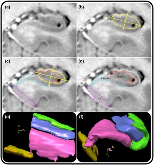
Illustration of the anatomic‐geometric heuristic for manual morphometry. (a) A representative slice of anterior hippocampal body following the visualization of the uncal sulcus. To facilitate tracing, the T₂‐weighted contrast has been inverted to mimic a T₁‐weighted image. (b) Placement of the ellipse and bisecting lines (the major and minor axes of the ellipse). (c) The minor axis bisecting the ellipse marks the point from which a vertical line is dropped to create a boundary separating the subiculum from CA1/2, and CA 1/2 from CA3–4/DG, as shown in (d). Bottom: 3‐D illustrations of sagittal (e) and oblique coronal (f) views of manual subfield labeling in the HC body from one EL participant [Color figure can be viewed at http://wileyonlinelibrary.com]

Following training, two separate operators manually traced the same sample of 12 cases (independent from the EL and LL samples but pooled from data acquired with identical acquisition properties) to assess inter‐rater agreement by computing intraclass correlation coefficients (ICC[2], for random raters; Shrout & Fleiss, 1979). For all regions, ICC(2) values of at least 0.85 for left and right hemispheres, separately, and at least 0.90 bilaterally were set as a benchmark for desired inter‐rater agreement. The same raters ranged slices, although one (AK) determined the ranges for the EL sample, whereas the other (ARB) determined the ranges for LL sample. The same two expert operators manually demarcated all images using these procedures, with randomized assignment of each slice to a given rater. Following a previously described procedure (Raz et al., 2004), the goal of slice assignment randomization between raters was to reduce the error of measurement.

2.4. Automated hippocampal segmentations

2.4.1. Atlas‐building

ASHS software (Yushkevich et al., 2015b) was used for atlas building following published procedures (https://sites.google.com/site/hipposubfields/building-an-atlas), without slice heuristics or cross‐validation procedures, as preliminary attempts to include slice heuristics produced multiple errors that diminished correspondence with manually demarcated data. These errors included partial or inaccurate segmentation of anterior and posterior regions, exclusion of multiple anterior and posterior slices, or spurious inclusion of regions on slices. Atlas building specified inclusion of four ROIs, consistent with the segmentation protocol. ROIs were exported from Analyze software to NIfTI format, and associated required MPRAGE data were converted to NIfTI from DICOM format. We initially created two separate, sample‐specific atlases for the EL and LL samples, respectively, as well as a lifespan atlas including manually demarcated data from both groups. Procedures published on the ASHS website (https://sites.google.com/site/hipposubfields/building-an-atlas; accessed December 16, 2016) recommend 20–30 cases for atlas building, and suggest that variations on this number still require additional validation to test any benefit of including additional data. Atlas building in ASHS was performed on a cluster‐computing environment running on Intel Xeon CPU ES‐2670 CPU cores running on Dell M620 blade servers, using the portable batch system for job scheduling.

2.4.2. Atlas building samples

ERC and HC subfields were ranged and manually demarcated on 100 participants, including 50 EL, and 50 LL. From each group, segmentations from 30 participants were assigned for atlas building, and the remaining 20 cases were used for ASHS segmentation and comparison with automated output. Assignment for atlas vs. segmentations was pseudorandomized to include similar age distributions in both atlas building and segmentation. No cases were used for both atlas building and procedure comparison.

The EL sample‐specific atlas included 30 children and adolescents (n = 20; age range = 6–14 years; mean age = 9.93, SD = 2.53 years; 50% female), and young adults (n = 10; age range = 18–24 years; mean age = 22.20, SD = 2.35 years; 50% female). The sample‐specific atlas for the LL sample included 28 older participants (age range = 62–79 years; mean age = 69.82, SD = 4.40 years; n female = 13), following exclusion of two cases (1 female, 68 years old; 1 female 71 years old) stemming from errors during atlas building due to these cases having an additional slice included during acquisition. We also used data from the EL and LL samples to build a third atlas spanning the entire age‐range of our sample. We designed the lifespan atlas to be composed of equal numbers of cases from the EL and LL samples. Because HC subfield volumes in young adults are more similar in size to older adults than to children (Daugherty et al., 2016), we weighted the EL cases more heavily for children and adolescents than for young adults. Thus, the lifespan atlas included data from 10 children and adolescents (age range = 7–13 years; mean age = 10.08, SD = 2.64 years; 50% female), four young adults (age range = 22–24 years; mean age = 23.00, SD = 0.82 years; 50% female), and 14 older adults (age range = 62–78 years; mean age = 69.64, SD = 4.63 years; 50% female).

2.4.3. ASHS segmentation using customized atlases

ASHS segmentation was applied to each sample using the age‐appropriate customized atlases as well as the combined lifespan atlas. The remaining 20 cases for each sample, whose ROIs were manually traced, but not used in atlas building, were used as validation cases. These were segmented using ASHS on the cluster‐computing environment described above.

2.5. Optimization by extending range of tracing

Following initial segmentation in ASHS, we examined the results, quantitatively and visually. Discrepancies between automated and manually demarcated image maps appeared most prominent at the first and final slices of all regions. In multiple cases, ASHS excluded segmentations for one or more ROIs on the first or final slices, or included additional slices that were not part of the manually ranged data. These issues could have plausibly arisen from imperfect registration of the T₁ and T₂‐weighted data, differences in angle of acquisition plane between the two, or a combination of these factors. Alternatively, it is possible that such differences arise because ASHS functions under an essentially different set of assumptions than manual raters (i.e., spatial and intensity values vs anatomical landmarks) when determining the longitudinal extent of segmentation.

To address these discrepancies, we modified the ranging rules, extending the ranges beyond manually designated anatomical landmarks for segmentation procedures used for images included for atlas building (Supporting Information, Figure SI1). This step was intended to reduce the likelihood of excluding anterior or posterior slices output during ASHS segmentation by producing an atlas that extended beyond anatomical ranges for manual inclusion. In this modified procedure, we traced additional slices: one to two anterior and one to two posterior slices were added to the manually defined ranges, depending on visibility of subfields. In anterior slices, any visible tissue from the uncus or the HC head was not included and demarcation was limited to clearly apparent HC “body‐like” regions on slices anterior to the uncal apex. On additional posterior slices, tracing was not performed in two cases, which showed no visible separation between the subfields. The extended ROIs were used for atlas building in ASHS following the same published guidelines, producing two extended sample‐specific atlases and one extended lifespan atlas. We then used the resultant extended, customized atlases in ASHS to segment the same 20 validation cases.

Initially, the extended demarcation was limited to the subfields in the HC body. However, this did not ameliorate problems in ERC measurements, with several cases showing pronounced ERC segmentation errors in more posterior slices of that structure. Therefore, an additional extended atlas that included expanded demarcation of that structure on additional posterior slices was generated. The final customized atlases in ASHS, with extended demarcation of both ERC and body subfields was again applied for segmentation of the 20 validation cases (see Figure 2 for a list of all atlases generated). Following ASHS segmentation, the extended validation data were truncated using an automated Bourne shell script and utilities from FSL v5.0 (Jenkinson, Beckmann, Behrens, Woolrich, & Smith, 2012) to limit ROIs to only those slices included in the manually defined ranges employed in the manual demarcation. Thus, operator‐determined ranges were preserved and ASHS propensity for segmentation problems at the anterior and posterior limits of the hippocampal body was kept in check. An additional inspection following the optimization determined whether the procedure successfully addressed the discrepancies. Following optimization, we observed three cases with minor segmentation errors on the most posterior HC body slice. However, following consultation between the operators responsible for ranging, demarcation, and optimization (ARB and AK), the additional error from those cases was deemed minimal and required no further correction. The raters noted, nonetheless, that in some cases it might have been preferable to use a more conservative criterion for the posterior HC body boundary, and adjust it to one slice anterior to the final slice on which LQ is visible.

Figure 2.

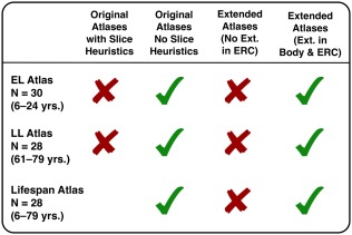
List of atlases generated and applied at different stages of validation work. Red Xs indicate atlases used at intermediate stages of the validation efforts, and green check marks indicate atlases used in reported analyses. The original atlases generated with the “slice heuristics” function in ASHS was only performed on the EL and LL samples, with no lifespan atlas generated. The optimization procedure included demarcation of subfields on one to two slices anterior and posterior, and was originally limited only to subfields and not ERC. Following inspection of the output from that atlas, additional demarcation was performed to similarly extend the labeling of ERC as well [Color figure can be viewed at http://wileyonlinelibrary.com]

2.6. Postoptimization correction

Following optimization procedures, we roughly estimated automated segmentation accuracy by comparing the total number of voxels and visually inspecting the manual and automated segmentation output. For ERC in the LL sample, we noted systematic differences: manual morphometry produced smaller volumes than ASHS did; however, no such systematic differences were apparent for ERC in the EL sample. Visual comparison of automated and manual masks revealed inconsistencies between the methods in 13 out of 20 cases for left‐only (n = 4), right‐only (n = 4), or bilateral ERC (n = 5). Consultation between the expert operators suggested that the smaller manually segmented ERC resulted from tendencies toward exceedingly conservative estimation of ERC in morphologically ambiguous circumstances, in which inferior termination points of demarcation were prescribed based on the appearance of false sulci, rather than at true collateral sulci. Based on this comparison, one rater (AK) manually corrected ERC for these 13 cases, blinded to automated output during correction procedures. Thus, corrections were only performed as indicated by apparent anatomical boundaries, and were not influenced by direct comparison with automated segmentations.

2.7. Data analysis

2.7.1. Inter‐rater agreement

Two complimentary indices of inter‐rater agreement and spatial overlap were used to evaluate the correspondence of manual and automated segmentations. The ICC(2) statistic (Shrout & Fleiss, 1979) is an analysis‐of‐variance‐based statistic that separates true variability of raters and volume differences from error, and thereby provides an estimate of bias in ratings. ICC(2) is geared towards assessing reliability of the volumes, the target measure in all studies cited above. It is not meant, however, to assess spatial overlap between geometric objects. When such overlap is of interest, the Dice similarity coefficient (DSC; Dice, 1945) is a statistic of choice. Although it gauges the spatial similarity or overlap of regions, DSC does not account for error variance in agreement, as it relies on set theory to evaluate overlap and commonality. Because the range truncation frequently resulted in differential number of slices between left and right hemispheres, mean DSC values following optimization were computed separately for each hemisphere, and bilateral DSC values after optimization were calculated as a mean across the hemispheres.

2.7.2. Bias estimation

ICC(2) is affected by the range of measured values, and a method less dependent on range is desirable. Therefore, we generated BA plots of agreement (Bland & Altman, 1986), which compare the differences between methods against their combined mean values. BA plots provide two useful indices: constant bias, which represents the departure of the differences between methods from zero, and proportional bias that indicates the association between bias and regional size, and are considered a standard in method comparison studies.

3. RESULTS

3.1. Ranging

The average number of slices used for manual demarcation of HC subfields differed between the samples. In the LL sample, the range contained one additional slice compared to the EL sample: mean (±SD) of the LL sample = 8.77 ± 0.92 slices; mean (±SD) of the EL sample = 7.82 ± 0.90 slices; t[98] = 5.24, p < .001.

3.2. Initial validation attempt

3.2.1. ICC(2)

The results of all validation attempts are presented in Table 1, and are depicted in Figure 3. For the EL sample, both the sample‐specific and Lifespan atlases showed low correspondence with manually demarcated data for ERC and SUB, and somewhat closer correspondence for CA1/2 and CA3/DG. The LL sample evidenced higher correspondence between manually traced and ASHS‐segmented subfield volumes. As with the EL sample, ERC for the LL sample showed the lowest agreement between manual and automated methods among all ROIs, regardless of the atlas used.

Table 1.

ICC(2) and DSC values for all segmentation attempts by atlas type and optimization for EL and LL samples

	EC left	EC right	EC total	EC left (corrected)	EC right (corrected)	EC total (corrected)	SUB left	SUB right	SUB total	CA1/2 left	CA1/2 right	CA1/2 total	CA3/DG left	CA3/DG right	CA3/DG total
LL sample ICC(2)
Sample specific, not optimized	0.686	0.455	0.502	0.660	0.424	0.478	0.859	0.406	0.717	0.623	0.732	0.716	0.822	0.727	0.806
Lifespan, not optimized	0.138	0.417	0.430	0.353	0.387	0.433	0.669	0.393	0.500	0.687	0.718	0.704	0.785	0.753	0.789
Sample specific, optimized	0.260	0.440	0.290	0.207	0.338	0.220	0.858	0.778	0.785	0.892	0.888	0.900	0.917	0.905	0.912
Lifespan, optimized	0.142	0.771	0.563	0.616	0.823	0.818	0.954	0.959	0.960	0.903	0.935	0.956	0.971	0.973	0.974
EL sample ICC(2)
Sample specific, not optimized	0.276	0.347	0.218				0.554	0.517	0.524	0.597	0.528	0.580	0.689	0.674	0.708
Lifespan, not optimized	0.429	0.158	0.180				0.441	0.491	0.458	0.757	0.632	0.743	0.757	0.762	0.794
Sample specific, optimized	0.603	0.594	0.556				0.933	0.859	0.912	0.913	0.679	0.839	0.939	0.800	0.894
Lifespan, optimized	0.658	0.674	0.635				0.938	0.855	0.900	0.885	0.688	0.840	0.953	0.844	0.923
LL sample DSC
Sample specific, not optimized	0.706	0.701	0.705			0.705	0.800	0.787	0.794	0.786	0.782	0.784	0.841	0.813	0.828
Lifespan, not optimized	0.702	0.695	0.698			0.698	0.785	0.775	0.780	0.771	0.767	0.769	0.818	0.810	0.814
Sample specific, optimized	0.746	0.763	0.755	0.747	0.764	0.755	0.842	0.841	0.842	0.824	0.839	0.832	0.878	0.877	0.878
Lifespan, optimized	0.801	0.817	0.809	0.817	0.824	0.820	0.835	0.840	0.837	0.828	0.837	0.833	0.873	0.872	0.873
EL sample DSC
Sample specific, not optimized	0.739	0.735	0.737				0.802	0.789	0.796	0.824	0.820	0.822	0.786	0.783	0.785
Lifespan, not optimized	0.736	0.722	0.730				0.801	0.786	0.794	0.824	0.817	0.821	0.780	0.768	0.774
Sample specific, optimized	0.825	0.805	0.815				0.853	0.842	0.848	0.888	0.884	0.886	0.848	0.847	0.847
Lifespan, optimized	0.820	0.816	0.818				0.847	0.841	0.844	0.887	0.889	0.888	0.844	0.845	0.845

Figure 3.

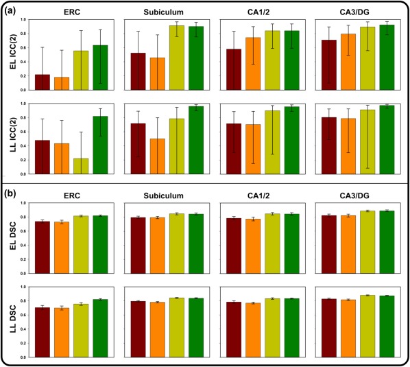
Results of validation attempts for four comparisons between manual and automated approaches in ASHS, including the sample‐specific atlas without optimization (red), the Lifespan atlas without optimization (orange), the sample‐specific atlas following optimization (yellow), and the Lifespan atlas following optimization (green). Error bars represent 95% confidence intervals. (a) ICC(2) values for the Early Lifespan sample (top) and the Late Lifespan sample (bottom). (b) DSC values for the Early Lifespan sample (top) and the Late Lifespan sample (bottom) [Color figure can be viewed at http://wileyonlinelibrary.com]

3.2.2. DSC

In contrast to the ICC(2) results, evaluation of DSC overlap between ASHS and manually demarcated data showed reasonable consistency between methods for both the EL and LL samples. However, the pattern of overlap loosely mirrored the ICC(2) results for both sample‐specific and Lifespan atlases, with lowest correspondence for ERC compared to other ROIs.

3.2.3. Visual inspection

In both the EL and LL samples, we observed consistent problems with ASHS segmentation, independent of the atlas used. These problems included a variety of segmentation errors that were primarily apparent at the most anterior and posterior aspects of ERC and the HC body. Segmentation errors were primarily defined by inclusion of extra voxels or mis‐segmentation of subfields in anterior or posterior slices by over‐ or underinclusion of relevant voxels (Figure 4). We observed one or more of such errors in almost all cases in both EL and LL samples. For the EL sample, problems with the initial ASHS segmentation were observed in ERC and in both the anterior and posterior HC body segmentations. ERC segmentation errors from ASHS output were observed in all EL cases, with 90% of validation cases showing bilateral ERC segmentation errors, and 10% only showing problems in the left or right ERC. Anterior HC body segmentation errors were also observed in 90% of the EL sample, with 15% of the brains showing unilateral and 75% of bilateral segmentation errors. Problems with posterior HC body segmentation were observed in 80% of cases, including 35% unilaterally, and 45% bilaterally.

Figure 4.

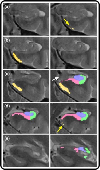
Illustration of ASHS segmentation errors in the initial, nonoptimized validation attempt. Left column depicts correct, manual segmentation, and right column shows faulty segmentations. (a) Whereas manual segmentation (left) does not include this slice in the range, ASHS (right) includes multiple, erroneously included voxels in ERC, as indicated by the yellow arrow. (b) Manual segmentation of ERC (left) in comparison with omitted segmentation by ASHS (right). (c) Manual segmentation includes only ERC (left) as visible presence of uncus (indicated by the white arrow) indicates no body segmentation on this slice. In contrast, ASHS (right) includes segmentation of ERC and body subregions. (d) Overextension of ERC by ASHS in several voxels (right, as indicated by the yellow arrow), where ERC should no longer be segmented following the first body slice (left). (e) Following the disappearance of the lamina quadrigemina, subfields are no longer segmented by the manual approach (left), but are both included, and mis‐segmented by ASHS (right) [Color figure can be viewed at http://wileyonlinelibrary.com]

In the LL sample, ERC segmentation errors from ASHS output were manifest in all cases, with 20% restricted to one hemisphere, and 80% showing problems bilaterally. Similarly, anterior HC body ASHS segmentation errors were ubiquitous, with errors in only one case restricted to the left hemisphere of the anterior HC body. Posterior HC body segmentation errors from ASHS were observed in 90% of those cases, with 25% showing improper segmentation unilaterally.

3.3. Postoptimization validation

3.3.1. ICC(2)

For the EL sample, postoptimization ICC(2) values revealed substantially improved automated‐manual correspondence for HC subfields in sample‐specific and Lifespan atlases. Although correspondence for ERC also improved, the higher validity coefficient (ICC[2] = 0.635) was still below the preestablished standard of inter‐rater reliability (i.e., 0.85). Bilateral ICC(2) values for SUB and CA3/DG approached or were above 0.90, but the ICC(2) for CA1/2, for both sample‐specific and Lifespan atlases was still lower than we hoped. In contrast, for the LL sample, the ICC(2) values for ERC were not considerably improved by optimization procedures. Correspondence between manually traced bilateral ERC and the sample‐specific atlas segmentation was only ICC(2) = 0.207, whereas the agreement between manual segmentation and the one produced by the Lifespan atlas reached a moderate value: ICC(2) = 0.590. Comparison of volumetric data and visual inspection revealed inconsistencies in several cases used in ERC atlas building, suggesting that ASHS segmentation output was more consistent than manual demarcation in this more ambiguous anatomical region in which no geometric‐anatomical heuristic was applied. Following correction of these 13 cases of manually demarcated ERC from the LL sample, the automated‐manual correspondence improved substantially for the Lifespan atlas, but not the sample‐specific atlas (Table 1). Similarly, concurrent validity for the remaining HC subfields SUB, CA1/2, and CA3/DG all showed marked improvements following optimization, with consistently higher ICC(2) values for the Lifespan than the sample‐specific atlas.

3.3.2. DSC

Spatial overlap between automated and manually segmented data increased following optimization procedures for both samples. This change was independent of atlas type. In addition, the differences between automated and manually segmented subfield data are most apparent at the edges of the structures (Figure 5), and some differences in the SUB‐CA1/2 boundary appear to differ in the anterior vs. posterior HC body.

Figure 5.

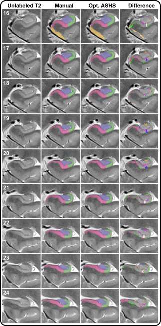
Illustration of labeling by manual demarcation, optimized ASHS in the lifespan atlas, and the difference between the two. Numbers in white represent z‐axis/slice number. The leftmost column shows the unlabeled T₂‐weighted, high‐resolution image on all slices included in manual labeling. Although this reflects the original contrast, manually demarcation was performed on images with inverted contrast (T₁‐weighted appearance). The middle columns show manual and automated demarcation of ERC and hippocampal subfields. The rightmost column shows the difference between ASHS and manual segmentation, and was generated by image subtraction between the two methods. As illustrated by the difference images (right column), the discrepancies between the two methods are most apparent at the edges of the subregional labels [Color figure can be viewed at http://wileyonlinelibrary.com]

3.3.3. Bias estimation

To evaluate whether one of the automated methods systematically under‐ or overestimates subfield volumes in comparison with manual morphometry, we generated BA plots (Figure 6 and Supporting Information, Figures 2 and 3). BA plots comparing ASHS automated output derived from sample‐specific and lifespan atlases, without optimization (Supporting Information, Figure 3) demonstrate a proportional bias in some regions: larger volumes were associated with greater negative differences, that is, smaller estimates generated by ASHS. In an extreme example, the proportional bias stemmed from one case from the LL sample having a large overall volume. In that case, ASHS did not adequately segment the first HC body slice on the left or the final HC body slice on the right, even following optimization procedures. This proportional bias appeared considerably greater in ERC and SUB than in CA1/2 and CA3/DG, and was reduced, though not eliminated, by optimization, particularly for the lifespan atlas (Figure 5).

Figure 6.

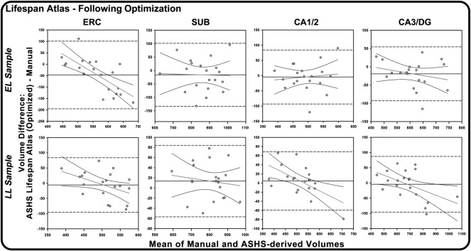
Bland‐Altman plots of agreement between manual and automated methods for Early Lifespan (EL) and Late Lifespan (LL) samples, using the ASHS customized lifespan atlas, following optimization procedures, with regression lines fitted to the data. On all plots, the Y‐axis represents the difference between ASHS automated and manual morphometry and the X‐axis represents the combined mean of the two methods. The solid black horizontal lines indicate the mean difference between methods, and the dashed lines represent the 95% confidence interval or two standard deviations above and below the mean difference. Negative regression slopes indicate proportional bias: the automatic procedure overestimates smaller volumes and underestimated the larger volumes, relative to manual segmentation

4. CROSS‐VALIDATION

To validate the optimization approach presented here, we applied it to an independent sample. The participants in that sample were recruited from a different population, and scanned on a different MRI installation, with some differences in acquisition parameters. The images were manually demarcated by independent raters who were trained on the manual segmentation protocol, described above. The data were also segmented in ASHS using the extended lifespan atlas optimized for limiting segmentations to the manually indicated slice ranges.

5. METHODS

5.1. Participants

The cross‐validation sample was drawn from ongoing, longitudinal investigations of brain and cognitive aging in Detroit, Michigan. Participants provided written informed consent in accord with the Declaration of Helsinki. The sample included 30 healthy adults (14 men and 16 women) from 31 to 84 years of age (mean age = 61.44, SD = 12.78 years). All participants were right‐handed, free of neurological and psychiatric diseases, and cognitively intact (MMSE range 26–30; mean MMSE = 29.20; SD = 1.03).

5.2. MRI acquisition

All sequences were acquired on a 3T Siemens Verio (Siemens Medical AG, Erlangen, Germany) MRI scanner with a 12‐channel head coil. We acquired a high‐resolution PD‐weighted TSE sequence in the coronal plane, perpendicular to the long axis of the hippocampus: TE = 17 ms, TR = 7150 ms, flip angle = 120°, pixel bandwidth = 96 Hz/pixel, turbo factor 11, in‐plain resolution = 0.4 mm × 0.4 mm, slice thickness = 2.0 mm, 30 slices, image matrix 280 × 512. Acquisition also included a high‐resolution T₁‐weighted MPRAGE sequence in the coronal plane, along the AC‐PC line, with TR = 1680 ms, TE = 3.51 ms, TI = 900 ms, flip angle = 9.0°, bandwidth = 180 Hz/pixel, GRAPPA acceleration factor 2, and voxel size = 0.67 mm × 0.67 mm × 1.34 mm.

5.3. Manual demarcation procedure

Manual demarcation was performed primarily by two raters (AMD and QY), using the same manual segmentation protocol as described above for the initial validation. The raters attained the same standards of reliability (ICC ≥ .90 for bilateral regions) and AMD was reliable with one of the raters who traced the original sample (ARB).

5.4. Automated segmentation and optimization

We used the extended‐lifespan atlas for segmentation in ASHS, followed by our optimization approach using the truncation procedure described above. Visual and quantitative inspection of the output showed disagreement in 12 out of 30 cases on the final body slice included in manual ranging. Thus, a somewhat more conservative range was applied, with the most posterior body slice excluded from the original ranging criteria.

6. RESULTS

Comparison between automated and manual segmentation showed high agreement, which was improved by applying a more conservative ranging criterion (Table 2). In addition, we identified an outlier with a very large hippocampus that was not segmented by ASHS on the two most anterior slices (Supporting Information, Figure 1). The influence of that outlier attenuated the validity coefficient for CA1/2. Overall, however, correspondence between the optimized ASHS output and manual segmentations was good, with ICC(2) values for bilateral ROIs ranging from 0.700 to 0.915.

Table 2.

Validity coefficients for cross‐validation

	ICC(2)
HC structure	Truncated	Truncated‐1+
ERC left	0.746	0.746
ERC right	0.697	0.697
ERC total	0.700	0.700
SUB left	0.885	0.923
SUB right	0.838	0.903
SUB total	0.857	0.915
CA1/2 left	0.707	0.815
CA1/2 righta	0.794	0.874
CA1/2 totala	0.807	0.876
CA3/DG left	0.854	0.905
CA3/DG right	0.824	0.873
CA3/DG total	0.858	0.905

^aExcluding 1 outlier; +Truncated to exclude one additional posterior body slice.

7. DISCUSSION

This study yielded four main results. First, we successfully created a series of customized atlases in ASHS using data from across the lifespan. This work extends prior findings from older adults (Yushkevich et al., 2015b) to children, adolescents, and younger adults using highly validated aggregated labels that have shown strong replicability across laboratories (Bender et al., 2013; Mueller et al., 2007; Mueller & Weiner, 2009; Shing et al., 2011). Second, we provided independent estimates of concurrent validity for ASHS segmentation of HC subfields based on novel customized atlases. Third, we showed that the concurrent validity and proportional bias of automated and manual HC subfield segmentation could be improved considerably by manually optimizing automated procedures and by using a lifespan sample for atlas generation, particularly for the LL sample. The optimization procedure used here is similar to that from the original ASHS work (Yushkevich et al., 2010), and relies on extending the boundaries during atlas building and truncating the data in accord with manual ranging criteria for slice inclusion. Fourth, we cross‐validated our findings. We replicated the concurrent validity findings based on the lifespan atlas and new optimization method on a sample from a different scanner, with different acquisition parameters, in a different population, demarcated by different raters trained on the same manual segmentation protocol.

7.1. Discrepancies: Sources and solutions

Automated approaches are highly consistent, but their external validity remains unknown until their output is carefully compared to the results of reliable manual tracing. The greatest disagreement in segmentation accuracy during the initial validation attempt arose in the most posterior or anterior aspects of cortex or subfields. An apparent strength of ASHS is in its excellent correspondence based on within‐slice segmentation. It encounters, nonetheless, problems in generalizing the longitudinal spatial extent from the training atlases to the target images. Left unchecked, ASHS may misclassify or exclude some or all regions in final slices, or, in some cases, add slices, relative to the range defined and segmented by the manual segmentation protocol, on which the customized atlases were based. Applying the ASHS “slice heuristics” function in atlas building did not remedy these discrepancies between manually defined ranges and the range of slices determined by ASHS. Whereas these discrepancies may produce similar estimations of total volume, they suggest a greater concern with specificity in coverage of the HC body. Furthermore, although these discrepancies were still apparent in applying our extended atlas and optimization procedures to an independent data set, this was remedied by applying a slightly more conservative criterion for range of slices included in estimating HC body volume.

Using BA plots, we found that ASHS produces a significant compression of variance in regional volumes, as the worst agreement with manual tracing was observed for extreme values. Similar variance compression has been observed when other automated procedures were compared to manual morphometry (e.g., Kennedy et al. 2009). This may be due to segmentation algorithms assuming that individuals are drawn from a homogenous, normally distributed population. The ensuing emphasis on central tendency may yield stronger influence on extreme cases by pulling those closer to the distribution mean. The MASV method employed in ASHS (Rohlfing et al., 2004; Klein and Hirsch, 2005), entails registration and normalization of individual native space images to a series of manually segmented template images, and subsequent inverse registration of multiple template‐based segmentations back to each individual image. A voting scheme is then used to combine the resultant multiple segmentations into a unified segmentation. The benefit of the MASV method in ASHS might have mitigated the deviations in atlas‐based segmentation within slices included in manually defined ranges.

We found that our optimization procedure that applied identical anatomical criteria used in manual segmentations to establishing regional inclusion boundaries improves the validity of automated approaches. Thus, the discrepancy in selection of multiple anatomical landmarks for establishing regional boundaries appears to be a crucial difference between manual and automated methods. However, even under the optimized procedures, the largest HC in the sample was still not correctly segmented, with the most anterior and posterior slices misclassified or not included. This may indicate a need for further refinement of HC body ranging procedures for both manual and automated segmentation methods (Wisse et al., 2017).

In addition, manual HC subfield demarcation has most frequently relied on widely used atlases, in which, unlike most MRI‐based segmentations, the slices are not aligned perpendicularly to the long axis of the hippocampus (Duvernoy, 2005). Manual methods involve the successive segmentation of structures on 2D slices and rely on multiple anatomical landmarks for determining range of inclusion and placement of internal boundaries. As such, manual demarcation benefits from expertise and recognition of relevant individual differences in brain morphology and standardized decision processes for handling partial volume effects or motion artifacts in structures of interest (i.e., CSF, GM/WM, dura, choroid plexus, blood vessels, etc.). In contrast, automated methods commonly utilize multiple types of spatial transformations to bridge various imaging modalities with different acquisition planes, different voxel size and varying degree of voxel anisotropy. Moreover, such automated approaches may be less sensitive to individual differences in morphology and relative distance from anatomical landmarks. The borders of some regions (i.e., ERC) are inherently more ambiguous because of multiple sources of noise, even when viewed by expert raters. Nevertheless, manual tracing remains the standard not because it is infallible, but because it is performed by trained experts who are guided by knowledge of neuroanatomy, understanding of MRI artifacts, and flexibility in considering individual differences. The present findings also suggest that automated, multiatlas voting approaches may help guide experienced raters in morphologically ambiguous circumstances. Together these issues underscore the importance of expert review of segmentation accuracy and consistency.

7.2. Relation to other findings

It is important to note that ICC and DSC statistics, which are rarely compared directly, reveal different but complimentary results. The ICC(2), essentially an analysis‐of‐variance technique, is sensitive to deviations between cases and procedures (automated vs. manual), and can be interpreted as reflecting error variability between methods, relative to the overall variability within the sample. DSC, a measure of spatial overlap between two structures, does not account for non‐error individual variability in their size. As expected, compared to DSC, the ICC(2) was considerably more sensitive to variability, as shown by the larger and more variable confidence intervals for the latter. Also, in both samples, the CA1/2 and CA3/DG regions appeared less sensitive than SUB and ERC to differences in automated vs. manual segmentation. These observations are supported by the BA plots (Figure 6) and by the bias statistics (Figure 7), which show lower bias for the lifespan atlas and reduction in bias following optimization procedures. It should be noted that the BA plots are sensitive to bias that reflects systematic differences between methods and overall tendencies toward generating differences in segmentations proportional to the size of the structure. In contrast, the 95% confidence intervals around the ICC(2) reflects the uncertainty of the statistic at the population level, and indicates that 95% of estimated intervals would include the population parameter. Thus, the three statistics reported here (ICC[2], DSC, BA bias) are complementary, and reflect different aspects of agreement between methods.

Figure 7.

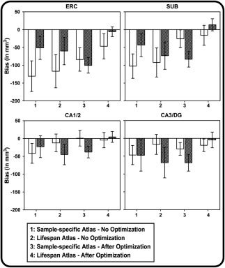
Comparison of bias from Bland–Altman plots across atlases, optimization methods, and HC subfields for Early lifespan sample (open bars) and the Late lifespan sample (filled bars). Error bars represent the 95% CI of the bias statistic

The present findings also highlight the greater difficulty of manual segmentation for ERC due to inconsistent interpretation of morphometric rules even by experienced raters. Moreover, as is apparent primarily in the LL sample, it is possible that this discrepancy resulted from differences in image acquisition or morphological differences in development. Indeed, in these images, both SUB and ERC were more likely than CA1/2 and CA3/DG influenced by differences in signal intensity arising from adjacent vasculature. This discrepancy also may result from poorer gray–white matter contrast, signal drop‐off, or partial voluming of subcortical white matter in rhinal cortices on 2‐mm thick slices used in our high‐resolution T₂‐weighted sequences, and typically employed in HC subfield imaging (Yushkevich et al., 2015a). These problems would be less likely on thinner T1‐weighted images with lower in‐plain resolution, on which EC volumes can be reliably estimated (e.g., Goncharova, Dickerson, Stoub, & deToledo‐Morrell, 2001; Raz et al., 2010). Together, these issues appear to make definitive manual designation of collateral sulcus more ambiguous (Insausti et al., 1998; Pruessner et al., 2002). However, the present findings may also indicate that use of the automated, MASV method by ASHS made it less vulnerable to imaging artifacts and partial voluming in comparison to expert manual operators. Although it can be performed reliably, ERC volume estimation is a challenging task even on thinner slices with isotropic voxels (e.g., Xu et al., 2000; Price et al., 2010). It remains unclear, pending comparison to histologically demarcated samples, whether this improvement in reliability also reflects greater validity of ERC demarcation by ASHS or greater consistency of the automated procedure.

7.3. Limitations and future directions

The results of this study should be interpreted in the context of several limitations. First, our segmentation was limited to the body of the HC and adjacent ERC and the results cannot be generalized to the hippocampal head and tail. Although ASHS may be capable of producing reliable segmentations of subfields in HC head and tail, histologically validated methods for cytoarchitectonically informed segmentation of subfields within HC head and tail are not yet established; this is primarily due to the less uniform distributions of subfields in the head and tail (Wisse et al., 2017). In the HC head, a challenge to validity emerges largely from its complex anatomical structure: the HC head is rotated in two planes and the number of HC head digitations can vary among individuals. Moreover, similarity of appearance displayed by tissue in the hippocampal head and amygdala on MRI can complicate precise, reliable demarcation of boundaries between adjacent gray matter regions. This is further complicated in aging samples as the age‐dependent inferior horn of the lateral ventricle frequently serves as a landmark for this boundary. This produces too many challenges to be treated without serious concerns about the differential distributions of subfields in the head (Wisse et al., 2017). In the tail, variability in acquisition angle, HC length, curvature, subfield distribution, and relative distance from the fornices and thalamus currently limits the validity of any segmentation protocol (Wisse et al., 2017). These challenges have been identified in enumerating the discrepancies among the protocols currently used for HC subfield demarcation (Yushkevich et al., 2015a) and the strategy towards improvement and harmonization of the rules are currently the goal of the Hippocampal Subfields Group consortium (Wisse et al., 2017).

Furthermore, several automated protocols offer segmentation with greater anatomical distinctions, yielding separate measures of almost all CA subregions, subiculum subregions, fimbria, alveus, the vestigial hippocampal fissure and the “dark band” on T2‐weighted, stratum radiatum lacunosum molecular (SRLM). As a rule, such highly specific labels show relatively low reliability in manual measures, and consequently low validity in automated protocols, whereas aggregating small regions improves both (Iglesias et al., 2015; Marizzoni et al., 2015; Yushkevich et al., 2015a). In contrast to this rule and to the pattern of results in the present study, a recent study of small, specific labels in five healthy adults showed high ICC, but lower DSC for SRLM (Amaral et al., 2017), although it is unclear which formula was used for ICC calculation, which limits direct comparison to the present study.

Second, our optimization procedure relies on manual intervention, as it involves defining HC body ranges based on anatomical landmarks. Consistent application of such procedures may be challenging for non‐expert human operators. In general, the various sources of potential discrepancies outlined above underscore the necessity of manually checking the output of automated segmentation protocols—although this is always strongly suggested when automated segmentation is performed. The benefit conveyed by removing an additional slice in the cross‐validation suggests that improving correspondence between manual and automated methods depends on accuracy of segmenting internal, within‐slice features and on consistent ranging. It remains unclear how representative are the individual slices along HC and whether including an entire region with a higher noise profile is preferable to more specific measures that sample a more limited, but representative anatomical aspect with smaller measurement error. Nevertheless, the optimization procedures described here and the manual inspection of automated output require certain expertise in MR‐based neuroanatomy. Thus, to attain the high levels of concurrent validity reported here, personnel charged with performing these steps should have adequate training and expertise in neuroanatomy. This is, of course, true with regards to any computerized procedure that benefits from corrections and adjustments to its automated output.

Third, the present validation was performed only with ASHS, and evaluation of other software for HC subfield segmentation was beyond the scope of the present study. Methods based on multi‐atlas segmentation, including Multiple Automatically Generated Templates brain segmentation (MAGeT‐Brain; Pipitone et al., 2014), should be evaluated. In addition, the Freesurfer software suite has included functionality for segmentation of HC subfields based on probabilistic or ex vivo data (Iglesias et al., 2015; Van Leemput et al., 2009). Although it is beyond the scope of the present study, additional work is also needed to reconcile the results of these approaches with the optimized morphometric approaches reported here.

Fourth, we combined the data from two independent studies, originally designed to investigate questions related to cognitive development and aging, respectively. While this, in part, motivated the division of data into EL and LL samples, it is possible that EL analysis might have benefitted from further subdivision into samples of children/adolescents versus young adults. Cross‐sectional evidence suggests that volumetric differences between children and early adulthood (Daugherty et al., 2016) vary across hippocampal subfields, and some young adults may more closely resemble their older counterparts than children. Sex differences in HC volume are reported in adolescence, with greater age‐associated decrements in total HC volumes in adolescent males compared to females (Satterthwaite et al., 2014). Furthermore, the two samples investigated in the present study were scanned with non‐identical acquisition methods and differed in averaging of multiple acquisitions and head coil used, which may complicate direct comparison of automated‐manual concurrent validity between groups. Thus, future studies should evaluate the differential utility of such automated, atlas‐based segmentation approaches for children and adolescents, by age and sex, while holding all other aspects of acquisition constant. Moreover, future studies should evaluate how well the optimization methods reported here extend to other data.

It is unclear why the lifespan atlases outperformed the sample‐specific atlases in their agreement with manually demarcated data. Considering the MASV approach used by ASHS, it may seem possible that the more variable set of atlas‐template images may have yielded a more diverse set of features, which ASHS could use to compare with any target image during segmentation. However, improving the concurrent validity of automated and manual segmentations by using the Lifespan rather than narrow‐age atlases is at odds with prior findings and theory (Wang et al., 2013). Although it is possible that agreement between manual and automated methods could have benefitted from uniform acquisition parameters, the present analyses suggest that greater variability in the data used for atlas building may improve correspondence. In the present study, we chose to build atlases based on age distributions, and not on specific morphological features such as HC size and shape. It is possible that the lifespan atlas outperformed the sample specific atlases because it included a greater distribution of such morphological features. Future validation efforts should compare the concurrent validity of automated segmentations from atlases built using age as a criterion with those specifically built to include a diverse set of morphological features. Similarly, the images for atlas building were chosen based, in part, on the relative absence of gross motion artifacts. Further validation is needed to determine the degree to which motion artifacts in atlas template images may influence segmentation accuracy. These results, however, highlight the need for further research to determine the conditions, under which a more variable training set yields segmentations with better correspondence with manual segmentations generated by a more uniform set of atlases.

It is also possible that ASHS segmentation errors at the most anterior or posterior aspects of the HC body stemmed from the manual segmentation protocol being limited to the body, at the exclusion of the head and tail. One might speculate that subfield segmentation along the full extent of the HC, or use of additional ROIs for total HC in head and tail may have possibly mitigated such errors. However, it is also possible that the ability of ASHS to clearly infer the anterior and posterior boundaries of HC body for subfield segmentation may not be as precise as that of manual raters. ASHS apparently does not consistently generalize internal boundaries along the longitudinal hippocampal axis from atlases to target data. This is a key concern for researchers attempting to limit ASHS segmentations to the body, or attempting to use a consistent and valid scheme for separate estimation of subfield volumes in the body, head, and tail. Thus, further work is needed to determine the exact causes and solutions for addressing these issues within the ASHS framework and to reduce or eliminate the need for manual intervention and optimization as described in the present study.

7.4. Conclusions

Within the ASHS automated pipeline, customized atlases can be used to reliably segment HC subfields in accord with evolving guidelines and protocols used in manual demarcation. Furthermore, using minimal manual interventions, automated output can be optimized to attain high correspondence with standard manual morphometric methods. These findings have strong implications for structural and functional studies of HC subfields, particularly in large datasets and for lifespan comparisons. The optimized segmentation procedure introduced here and reliance on a lifespan atlas eliminated constant bias of automatic vs. manual segmentation. Nonetheless, proportional bias in some subfields remained and further refinement of segmentation procedures and neuroanatomical validation of demarcation rules remains critically important for advancement of research that relies on HC subfield morphometry.

Supporting information

Additional Supporting Information may be found online in the supporting information tab for this article.

Figure SI1. Example of extended subfield demarcation scheme. Additional slices included in demarcation of body subfield ROIs in slices 15 (anterior) and 24 (posterior) are shown with a solid red outline, and additional posterior ERC on slices 17‐19 (dashed red outline).

Figure SI2. Bland‐Altman plots of agreement between manual and automated methods for Early Lifespan (EL) and Late Lifespan (LL) samples, using the ASHS customized sample‐specific atlases, following optimization procedures, with regression lines fitted to the data. On all plots, the Y‐axis represents the difference between ASHS automated and manual morphometry, and the X‐axis represents the combined mean of the two methods. The solid black horizontal lines indicate the mean difference between methods, and the dashed lines represent the 95% confidence interval or two standard deviations above and below the mean difference.

Figure SI3. Bland‐Altman plots of agreement between manual and automated methods for Early Lifespan (EL) and Late Lifespan (LL) samples, using the ASHS customized lifespan and sample‐specific atlases, with no optimization procedures applied. Regression lines are fitted to the data. On all plots, the Y‐axis represents the difference between ASHS automated and manual morphometry, and the X‐axis represents the combined mean of the two methods. The solid black horizontal lines indicate the mean difference between methods, and the dashed lines represent the 95% confidence interval or two standard deviations above and below the mean difference.

Bender AR, Keresztes A, Bodammer NC, et al. Optimization and validation of automated hippocampal subfield segmentation across the lifespan. Hum Brain Mapp. 2018;39:916–931. 10.1002/hbm.23891

REFERENCES

- Amaral, R. S. , Park, M. T. , Devenyi, G. A. , Lynn, V. , Pipitone, J. , Winterburn, J. , … Chakravarty, M. M. (2017). Manual segmentation of the fornix, fimbria, and alveus on high‐resolution 3T MRI: Application via fully‐automated mapping of the human memory circuit white and grey matter in healthy and pathological aging. NeuroImage. Available online Oct 18, 2016. [DOI] [PubMed] [Google Scholar]
- Bender, A. R. , Daugherty, A. M. , & Raz, N. (2013). Vascular risk moderates associations between hippocampal subfield volumes and memory. Journal of Cognitive Neuroscience, 25, 1851–1862. [DOI] [PubMed] [Google Scholar]
- Bertram, L. , Böckenhoff, A. , Demuth, I. , Düzel, S. , Eckardt, R. , Li, S. C. , … Steinhagen‐Thiessen, E. (2014). Cohort profile: The Berlin aging study II (BASE‐II). International Journal of Epidemiology, dyt018. [DOI] [PubMed] [Google Scholar]
- Bland, J. M. , & Altman, D. (1986). Statistical methods for assessing agreement between two methods of clinical measurement. Lancet, 327, 307–310. [PubMed] [Google Scholar]
- Crocker, L. , & Algina, J. (1986). Introduction to classical and modern test theory. Orlando, FL: Holt, Rinehart and Winston. [Google Scholar]
- Cronbach, L. J. , & Meehl, P. E. (1955). Construct validity in psychological tests. Psychological Bulletin, 52(4), 281–302. [DOI] [PubMed] [Google Scholar]
- Daugherty, A. M. , Yu, Q. , Flinn, R. , & Ofen, N. (2015). A reliable and valid method for manual demarcation of hippocampal head, body, and tail. International Journal of Developmental Neuroscience : The Official Journal of the International Society for Developmental Neuroscience, 41, 115–122. [DOI] [PubMed] [Google Scholar]
- Daugherty, A. M. , Bender, A. R. , Raz, N. , & Ofen, N. (2016). Age differences in hippocampal subfield volumes from childhood to late adulthood. Hippocampus, 26, 220–228. [DOI] [PMC free article] [PubMed] [Google Scholar]
- Dice, L. R. (1945). Measures of the amount of ecologic association between species. Ecology, 26, 297–302. [Google Scholar]
- Duvernoy, H. M. (2005). The human hippocampus: Functional anatomy, vascularization, and serial sections with MRI (3rd ed). Berlin, New York: Springer. [Google Scholar]
- Goncharova, I. I. , Dickerson, B. C. , Stoub, T. R. , & deToledo‐Morrell, L. (2001). MRI of human entorhinal cortex: A reliable protocol for volumetric measurement. Neurobiology of Aging, 22, 737–745. [DOI] [PubMed] [Google Scholar]
- Iglesias, J. E. , Augustinack, J. C. , Nguyen, K. , Player, C. M. , Player, A. , Wright, M. , … Fischl, B. (2015). A computational atlas of the hippocampal formation using ex vivo, ultra‐high resolution MRI: Application to adaptive segmentation of in vivo MRI. NeuroImage, 115, 117–137. [DOI] [PMC free article] [PubMed] [Google Scholar]
- Insausti, R. , Juottonen, K. , Soininen, H. , Insausti, A. M. , Partanen, K. , Vainio, P. , … Pitkänen, A. (1998). MR volumetric analysis of the human entorhinal, perirhinal, and temporopolar cortices. American Journal of Neuroradiology, 19, 659–671. [PMC free article] [PubMed] [Google Scholar]
- Jenkinson, M. , Bannister, P. , Brady, M. , & Smith, S. (2002). Improved optimization for the robust and accurate linear registration and motion correction of brain images. NeuroImage, 17, 825–841. [DOI] [PubMed] [Google Scholar]
- Jenkinson, M. , Beckmann, C. F. , Behrens, T. E. , Woolrich, M. W. , & Smith, S. M. (2012). FSL. NeuroImage, 62, 782–790. [DOI] [PubMed] [Google Scholar]
- Jenkinson, M. , & Smith, S. (2001). A global optimisation method for robust affine registration of brain images. Medical Image Analysis, 5, 143–156. [DOI] [PubMed] [Google Scholar]
- Kennedy, K. M. , Erickson, K. I. , Rodrigue, K. M. , Voss, M. W. , Colcombe, S. J. , Kramer, A. F. , … Raz, N. (2009). Age‐related differences in regional brain volumes: A comparison of optimized voxel‐based morphometry to manual volumetry. Neurobiology of Aging, 30, 1657–1676. [DOI] [PMC free article] [PubMed] [Google Scholar]
- Klein, A. , & Hirsch, J. (2005). Mindboggle: A scatterbrained approach to automate brain labeling. NeuroImage, 24, 261–280. [DOI] [PubMed] [Google Scholar]
- Marizzoni, M. , Antelmi, L. , Bosch, B. , Bartres‐Faz, D. , Muller, B. W. , Wiltfang, J. , … Jovicich, J. (2015). Longitudinal reproducibility of automatically segmented hippocampal subfields: A multisite European 3T study on healthy elderly. Human Brain Mapping, 36, 3516–3527. [DOI] [PMC free article] [PubMed] [Google Scholar]
- Mueller, S. G. , Stables, L. , Du, A. T. , Schuff, N. , Truran, D. , Cashdollar, N. , & Weiner, M. W. (2007). Measurement of hippocampal subfields and age‐related changes with high resolution MRI at 4 T. Neurobiology of Aging, 28, 719–726. [DOI] [PMC free article] [PubMed] [Google Scholar]
- Mueller, S. G. , & Weiner, M. W. (2009). Selective effect of age, Apo e4, and Alzheimer's disease on hippocampal subfields. Hippocampus, 19, 558–564. [DOI] [PMC free article] [PubMed] [Google Scholar]
- Ofen, N. , & Shing, Y. L. (2013). From perception to memory: Changes in memory systems across the lifespan. Neuroscience and Biobehavioral Reviews, 37, 2258–2267. [DOI] [PubMed] [Google Scholar]
- Price, C. C. , Wood, M. F. , Leonard, C. M. , Towler, S. , Ward, J. , Montijo, H. , … Schmalfuss, I. (2010). Entorhinal cortex volume in older adults: Reliability and validity considerations for three published measurement protocols. Journal of the International Neuropsychological Society, 16(5), 846–855. [DOI] [PMC free article] [PubMed] [Google Scholar]
- Pruessner, J. C. , Köhler, S. , Crane, J. , Pruessner, M. , Lord, C. , Byrne, A. , … Evans, A. C. (2002). Volumetry of temporopolar, perirhinal, entorhinal and parahippocampal cortex from high‐resolution MR images: Considering the variability of the collateral sulcus. Cerebral Cortex, 12, 1342–1353. [DOI] [PubMed] [Google Scholar]
- Raz, N. (2000). Aging of the brain and its impact on cognitive performance: Integration of structural and functional findings In Craik F.I.M. & Salthouse T.A. (Eds.), Handbook of aging and cognition ‐ II (pp. 1–90). Mahwah, NJ: Erlbaum. [Google Scholar]
- Raz, N. , Daugherty, A. M. , Bender, A. R. , Dahle, C. L. , & Land, S. (2015). Volume of the hippocampal subfields in healthy adults: Differential associations with age and a pro‐inflammatory genetic variant. Brain Structure and Function, 220, 2663–2674. [DOI] [PMC free article] [PubMed] [Google Scholar]
- Raz, N. , Gunning‐Dixon, F. , Head, D. , Williamson, A. , Rodrigue, K. , & Acker, J. D. (2004). Aging, sexual dimorphism, and hemispheric asymmetry of the cerebral cortex: Replicability of regional differences in volume. Neurobiology of Aging, 25, 377–396. [DOI] [PubMed] [Google Scholar]
- Rohlfing, T. , Brandt, R. , Menzel, R. , & Maurer, C. R. (2004). Evaluation of atlas selection strategies for atlas‐based image segmentation with application to confocal microscopy images of bee brains. NeuroImage, 21, 428–1442. [DOI] [PubMed] [Google Scholar]
- Satterthwaite, T. D. , Vandekar, S. , Wolf, D. H. , Ruparel, K. , Roalf, D. R. , Jackson, C. , … Davatzikos, C. (2014). Sex differences in the effect of puberty on hippocampal morphology. Journal of the American Academy of Child and Adolescent Psychiatry, 53, 341–350. [DOI] [PMC free article] [PubMed] [Google Scholar]
- Shing, Y. L. , Rodrigue, K. M. , Kennedy, K. M. , Fandakova, Y. , Bodammer, N. , Werkle‐Bergner, M. , … Raz, N. (2011). Hippocampal subfield volumes: Age, vascular risk, and correlation with associative memory. Frontiers in Aging Neuroscience, 3, 2. [DOI] [PMC free article] [PubMed] [Google Scholar]
- Shrout, P. E. , & Fleiss, J. L. (1979). Intraclass correlations: Uses in assessing rater reliability. Psychological Bulletin, 86, 420–428. [DOI] [PubMed] [Google Scholar]
- Small, S. A. , Schobel, S. A. , Buxton, R. B. , Witter, M. P. , & Barnes, C. A. (2011). A pathophysiological framework of hippocampal dysfunction in ageing and disease. Nature Reviews. Neuroscience, 12, 585–601. [DOI] [PMC free article] [PubMed] [Google Scholar]
- Wang, H. , Suh, J. W. , Das, S. R. , Pluta, J. B. , Craige, C. , & Yushkevich, P. A. (2013). Multi‐atlas segmentation with joint label fusion. IEEE Transactions on Pattern Analysis and Machine Intelligence, 35, 611–623. [DOI] [PMC free article] [PubMed] [Google Scholar]
- Wisse, L. E. M. , Daugherty, A. M. , Olsen, R. K. , Berron, D. , Carr, V. A. , Stark, C. E. L. , …. la Joie, R. for the Hippocampal Subfields Group . (2017). A harmonized segmentation protocol for hippocampal and parahippocampal subregions: Why do we need one and what are the key goals? Hippocampus, 27, 3–11. [DOI] [PMC free article] [PubMed] [Google Scholar]
- Xu, Y. , Jack, C. R., Jr , O'brien, P. C. , Kokmen, E. , Smith, G. E. , Ivnik, R. J. , … Petersen, R. C. (2000). Usefulness of MRI measures of entorhinal cortex versus hippocampus in AD. Neurology, 54, 1760–1767. [DOI] [PubMed] [Google Scholar]
- Yushkevich, P. A. , Wang, H. , Pluta, J. , Das, S. R. , Craige, C. , Avants, B. B. , … Mueller, S. (2010). Nearly automatic segmentation of hippocampal subfields in in vivo focal T2‐weighted MRI. NeuroImage, 53, 1208–1224. [DOI] [PMC free article] [PubMed] [Google Scholar]
- Yushkevich, P. A. , Amaral, R. S. , Augustinack, J. C. , Bender, A. R. , Bernstein, J. D. , Boccardi, M. … Hippocampal Subfields Group . (2015a). Quantitative comparison of 21 protocols for labeling hippocampal subfields and parahippocampal subregions in in vivo MRI: Towards a harmonized segmentation protocol. NeuroImage, 111, 526–541. [DOI] [PMC free article] [PubMed] [Google Scholar]
- Yushkevich, P. A. , Pluta, J. B. , Wang, H. , Xie, L. , Ding, S. L. , Gertje, E. C. , … Wolk, D. A. (2015b). Automated volumetry and regional thickness analysis of hippocampal subfields and medial temporal cortical structures in mild cognitive impairment. Human Brain Mapping, 36, 258–287. [DOI] [PMC free article] [PubMed] [Google Scholar]
Associated Data
This section collects any data citations, data availability statements, or supplementary materials included in this article.
Supplementary Materials