The University of Wisconsin Breast Cancer Epidemiology Simulation Model: An Update

Abstract

The University of Wisconsin Breast Cancer Epidemiology Simulation Model (UWBCS), also referred to as Model W, is a discrete-event microsimulation model that uses a systems engineering approach to replicate breast cancer epidemiology in the US over time. This population-based model simulates the lifetimes of individual women through four main model components: breast cancer natural history, detection, treatment, and mortality. A key feature of the UWBCS is that in addition to specifying a population distribution in tumor growth rates, the model allows for heterogeneity in tumor behavior, with some tumors having limited malignant potential (i.e., would never become fatal in a woman’s lifetime if left untreated) and some tumors to be very aggressive based on metastatic spread early in their onset. The model is calibrated to Surveillance, Epidemiology, and End Results (SEER) breast cancer incidence and mortality data from 1975–2010 and cross-validated against data from the Wisconsin cancer reporting system. The UWBCS model generates detailed outputs including underlying disease states and observed clinical outcomes by age and calendar year as well as costs, resource usage, and quality of life associated with screening and treatment. The UWBCS has been recently updated to account for differences in breast cancer detection, treatment and survival by molecular subtypes (defined by ER/ HER2 status), to reflect the recent advances in screening and treatment, and to consider a range of breast cancer risk factors including breast density, race, body-mass-index, and use of postmenopausal hormone therapy. Therefore the model is able to evaluate novel screening strategies such as risk-based screening and can assess breast cancer outcomes by breast cancer molecular subtype. In this article, we describe the most up-to-date version of the UWBCS.

1. Introduction

The University of Wisconsin Breast Cancer Epidemiology Simulation Model (UWBCS), also referred to as Model W was developed as part of the National Cancer Institute’s Cancer Intervention and Surveillance Modeling Network (CISNET) consortium. The UWBCS is a discrete-event microsimulation model that replicates breast cancer epidemiology in the U.S. over time.

The UWBCS was initially developed in the first round of CISNET funding (2000–2005) and was used to evaluate the impact of adjuvant therapy and screening mammography on U.S. breast cancer mortality between 1975 and 2000[1]. [1] The original UWBCS, which replicated U.S. stage-specific breast cancer incidence and overall breast cancer mortality between 1975 and 2000, has been described previously.[2, 3] Since then, the model has evolved with many changes in inputs and structure and has been extended to predict breast cancer epidemiology through 2010 and beyond. The purpose of this paper is to describe the model structure and natural history assumptions, calibration, and validation with attention to recent modifications.

Key recent modifications include:

1. The model’s inputs representing the utilization of screening mammography over time in the U.S. have been updated to replicate screening patterns through 2010 while accounting for the transition from film to digital mammography beginning in 2000.

2. Inputs for the accuracy of mammography haave been updated to include the contemporary performance of digital mammography according to age, breast density, and screening interval.

3. New advances in treatment such as aromatase inhibitors, taxanes, trastuzumab, have been incorporated into the model. The dissemination of all adjuvant treatment regimens over time has also been extended through 2010.

4. Treatment effectiveness inputs have been modified to account for recent studies reporting outcomes with newer regimens, as well as those reporting longer term outcomes among patients enrolled in older clinical trials

5. Breast cancer molecular subtype defined by human epidermal growth factor receptor 2 (HER2) was added to the model, which previously included only estrogen receptor (ER) subtype.

6. A risk-factor version of the model was developed which accounts for secular trends in breast cancer risk factors such as breast density, postmenopausal hormone therapy, and body mass index (BMI). There are two versions of the current model: one not including risk factors explicitly and one that includes risk factors.

7. A race-specific version of the model was developed in which black and white women are modeled separately with different parameters for natural histories, screening, and treatment components.

There are currently three versions of the UWBCS: base model, a risk-factor version of the model, and a race-specific model. Unless noted otherwise, we refer to the base model throughout this paper. We next describe the latest version of the model in more detail.

2. Model Overview

The UWBCS is a discrete-event system microsimulation model using discrete-time intervals (fixed cycles) of 6 months to represent breast cancer-related events. The UWBCS simulates women individually by birth cohort from age 20 until death. The model starts by simulating the cross-sectional female population in 1950. Each year after 1950, women who turn 20 are added to the model. The population sizes in 1950 and for subsequent years are estimated using U.S. census data. In 1950, the model assumes that all women are cancer-free. While the model starts simulating women in 1950, the first 25 years of simulated time (between 1950–1975) is used as the warm-up period for the simulation[4] to ensure that the model‐predicted prevalence of breast cancer in 1975 is similar to underlying prevalence of breast cancer in 1975. The model is then run forward to predict US trends.

Model inputs have been extended through 2010, and the model uses 2010 inputs for future years and projections. The UWBCS has been implemented in C++ containing over 20,000 lines of code. Each simulation of the US female population (1 simulated woman for each 50 US women) from 1950 to 2020 takes approximately 5 minutes without parallelization on a computer with an Intel i5 3210M processor.

The model simulates the lifetimes of individual women through four main model components: 1) breast cancer natural history component that simulates tumors from an unobservable size/stage until breast-cancer related death; 2) breast cancer detection component that represents screening and clinical surfacing; 3) breast cancer treatment component 4) other-cause mortality component that simulates deaths due to non-breast cancer causes. Briefly, each woman enters the model at age 20 and is assigned an initial risk factor profile based on population distributions and joint distributions if there are two or more non-independent risks for breast cancer. Figure 1 summarizes the steps each woman experiences every 6 months as she ages. Risk of breast cancer is a function of age, calendar year, and risk factors. If breast cancer develops, it progresses through disease stages following a stochastic growth curve. Cancer can be detected by clinical surfacing (symptomatically) or by screening; interval cancers are a subset of the clinically detected cases. Upon detection, stage-, and age-, calendar year- and tumor subtype- specific treatment is applied. Women with cancer are at risk of death from breast cancer while all women face competing mortality risks. We next describe each model component in more detail.

Figure 1.

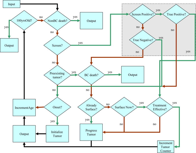
Simulation Flowchart of the UWBCS

3. Model Components

3.1. Natural History Component

Overall breast cancer incidence is a function of a woman’s birth year and age (as well as risk factors in risk-specific version and race in race-specific version) and accounts for secular trends in incidence and risk factors over time. Our cancer natural history makes several assumptions: 1) all cancers start at in situ stage (that includes ductal carcinoma in situ (DCIS) as well as non- DCIS in situ cancers) and that in situ cancer is a precursor to invasive cancer; 2) tumor size indicating cancer stage is represented using the shape of a perfect sphere, (i.e., tumor size is used as a proxy for cancer severity and progression); 3) a fraction of in situ and small invasive cancers never lead to breast cancer death; these are referred to as limited malignant potential (LMP) tumors; and 4) some cancers are hyperaggressive at the time of onset. Table 1 lists all of the natural history parameters used in the model. All of these parameters are estimated via calibration as explained in the next section.

Table 1.

Breast Cancer Natural History Input Parameters Estimated via Model Calibration and Their Best-fitting Values

Parameter Name	Description	Value in the “Best” Vector
LMP Fraction	Proportion of tumors with limited malignant potential (LMP)	42%
Max LMP size	The maximum size for LMP tumors	1 cm
LMP Dwell Time	After an LMP tumor reaches Max LMP size, this parameter represents the time for this LMP tumor to regress or become undetectable	2 years
Onset Proportion	Ratio of biologic onset rate of non LMP tumors to APC predicted incidence rate in the absence of screening	90%
Onset Lag	Time between APC predicted incidence of a tumor and the inception of the tumor in the model	3 years
Mean Gamma	Mean value of the Gompertzian tumor growth variable (α) that is distributed with Gamma distribution	0.12
Variance Growth	Variance of the Gompertzian tumor growth variable (α) that is distributed with Gamma distribution	0.012
In situ boundary	The diameter below which a tumor is classified as in situ cancer if no lymph nodes are involved	0.95 cm
Percent aggressive	Percentage of non LMP tumors that are classified as regional cancers at onset	1%
Percent highly aggressive	Percentage of non LMP tumors that are classified as distant cancers at onset	2%

Abbreviations: APC, age period cohort; LMP, limited malignant potential.

3.1.1. Cancer Onset

Cancer onset begins at a diameter of 2 mm, a size that is assumed to be undetectable by mammography. The onset of undetectable tumors is a function of expected incidence in the absence of screening as initially estimated by an age-period-cohort (APC) model by Holford et al.[5] and later updated by Gangnon et al.[6], a CISNET common input. Both APC models predict an increase in breast cancer incidence over time. We incorporate Holford’s APC model directly until 2000, and then for years after 2000, we extended the Holford’s APC model using the APC model of Gangnon et al.[6]

A key assumption in the UWBCS is the existence of “limited malignant potential” (LMP) tumors. LMP tumors were required to explain observed patterns of breast cancer incidence and mortality between 1975 and 2000.

The APC models provide the number of cancers that are onset per 100,000 women in a given year for a given birth cohort. Then, the total onset of cancers per 100,000 women in a year for a given birth cohort (BC) is estimated using the following equation [2]:

$$\mathit{Total}{\mathit{Onset}}_{\mathit{BC},\mathit{Y}+\mathit{Onset}\mathit{Lag}}=\mathit{AP}{\mathit{C}}_{\mathit{BC},\mathit{Y}+\mathit{Onset}\mathit{Lag}}\ast \mathit{Onset}\mathit{Proportion}\ast \frac{1}{1-\mathit{LMP}\mathit{Fraction}},$$

where APC_{BC, Y-Onset Lag} represents the incidence rate predicted by the APC model for women in this birth cohort in year Y + Onset Lag, Onset Proportion represents the ratio of onset of non- LMP tumors to APC- predicted incidence, LMP fraction represents the proportion of tumors that are of LMP type, and Onset Lag represents the time (in years) between the APC-predicted incidence rate and onset rate used in Onset Proportion that was added to allow a possible delay in the time from biological onset to the detection of the tumor by clinical surfacing or screening.[2] For example, suppose the APC model predicts 250 cancers per 100,000 women in year 1990 for 1950 birth cohort (women who were born in 1950), Onset Lag is 2 years, Onset Proportion is 80%, and LMP fraction is 50%, then 250*80%*2 = 400 cancers per 100,000 42- year-old women or thereabouts are initiated in 1992. If the cohort size for 1950 birth cohort is 2 million, then a total of approximately 400*20 = 8000 cancers are initiated for 1950 birth cohort in 1992. The total onset in year 1992 is equal to the summation of all cancer onsets for all birth cohorts in this year. In this equation, Onset Lag, Onset Proportion, and LMP fraction are all estimated via calibration.

3.1.2. Tumor Growth

After onset, each tumor is assumed to grow according to a stochastic Gompertz-type function: [7, 8]

$$N(t)=N(0)\mathit{exp}\lfloor \ln \left(\frac{\mathrm{N}(\infty )}{\mathrm{N}(0)}\right)(1-\mathit{exp}(-\alpha t))\rfloor ,$$

where N(t) represents the tumor size at time t, N(0) represents the initial tumor size (assumed to be 2 mm), N(∞) represents the maximum tumor size (assumed to be 8 cm), and α represents a tumor’s individual growth rate. The Gompertz function has decelerating growth. The growth parameter, α, is estimated from a population distribution of tumor growth rates that follows a Gamma distribution.[2] The mean and variance of α are estimated via calibration. Tumor growth rates do not depend on ER/HER2 in our model.

LMP tumors grow with the same rate as non-LMP tumors; stop growing at a small size (Max LMP size), that is estimated with calibration; and if undetected after a fixed length of time (LMP dwell time) that is also estimated via calibration, they become undetectable or regress. After an LMP tumor regresses or becomes undetectable, the woman becomes cancer-free and is again at risk for a new cancer onset. There is evidence in the breast cancer literature about the existence of LMP tumors. [9–13] As noted above, the fraction of LMP tumors at onset (LMP fraction) is also estimated via calibration.

3.1.3. Hyperaggressive Tumors

The model assumes that some non-LMP tumors progress very aggressively at the time of onset. These hyperaggressive tumors are assumed to spread to multiple lymph nodes at their onset and are therefore are classified as regional or distant stage but could be detected clinically or via screening. The spread of breast cancer to lymph nodes follows a Poisson process using two parameters: percent aggressive represents the percentage of non-LMP tumors that are classified as regional at onset and percent highly aggressive represents the percentage of non-LMP tumors classified as distant at onset.

3.1.4. Tumor Staging

The size of tumor and nodal status in the model provide a proxy for the severity of breast cancer in a woman and translate to one of four Surveillance, Epidemiology, and End Results (SEER) historical cancer stages: in situ, localized, regional, or distant (Figure 2). If no lymph nodes are involved, then there is a threshold tumor diameter below which a tumor is classified as in situ and over which it is classified as localized. This threshold tumor diameter, referred to as In situ boundary is estimated via calibration. A proportion of in situ cancers are also assigned as DCIS. We refer to SEER historical cancer staging throughout this paper unless noted otherwise.

Figure 2.

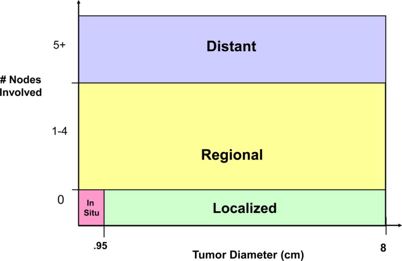
Translation of Tumor size and Nodal Involvement in the Model to SEER staging

3.1.5. Breast Cancer Death

If a tumor is not cured, it progresses to the distant stage and the woman is assigned a time of breast cancer death using the CISNET common input for ER/HER2 specific survival curves for distant stage.[14] The progression of uncured tumor to the distant stage (through local and regional stages) is governed by the natural history parameters. Breast cancer death occurs if the time of breast cancer death occurs before the time of death due to non-breast cancer reasons.

3.2. Breast Cancer Detection Component

Cancer detection can occur via routine screening or clinical surfacing that represents symptomatic detection via a clinical breast exam or a self-detection. We defined cancer detection with a probability that is a function of tumor size implying that the larger the tumor, the more likely it is to be detected via screening or clinical surfacing. For this purpose, for screening, we defined a piecewise-linear detection function over the tumor size that was divided into several cutoff points: 0–0.2 cm; 0.2–0.5 cm; 0.5 cm-0.75 cm; 0.75 cm- 1.5 cm; 1.5 cm-2 cm; 2 cm- 5 cm; 5 cm–8 cm. We assumed that the probability of detection is 0 when the tumor is between 0–0.2 cm, and it is equal to 0.99 and 1 when the tumor is 5 cm and 8 cm, respectively. For tumor sizes between 0.2 cm and 5 cm, the probability of detection is calibrated to match target mammography screening sensitivity values provided by the Breast Cancer Surveillance Consortium (BCSC) as a CISNET common input. Target sensitivity values can be defined as a function of breast density, screening round and interval between screens, and age group.

We assumed that the probability of detection function for clinical surfacing is always lower than that for screening, since screening typically detects cancers earlier than other detection methods such as self-detection or clinical breast exam. To reflect the changing mammography performance over time, we estimated different probability of detection functions for digital and film mammography. Furthermore, to reflect the improving accuracy of film mammography over time, we used different probability of detection functions for 1984 and 2000 and interpolated in between such that mammography accuracy improves over time. Moreover, to reflect the differences in mammography performance by age, we used different probability of detection functions for three age groups: <50, 50–64, and >65. Similarly, the probability of detection function for clinical surfacing was also different for years 1990 and 2000. The probability detection functions for clinical surfacing and screening were determined via calibration.

The UWBCS replicates the diffusion of film mammography over time beginning in the early 1980s using a mammography dissemination model developed as a CISNET common input parameter.[14] The model also represents the diffusion of digital mammography beginning in 2000s, provides as a CISNET common input.[14] The specificity of film and digital mammography were also provided by BCSC as a common input and are based on age, breast density, and screening interval.[14] The details for estimating these inputs as well as their values are available elsewhere. [14]

In addition to the replicating observed screening practices in the U.S., the UWBCS can also be used to simulate fixed screening scenarios by varying start and stopping ages and screening frequencies.

3.3. Breast Cancer Treatment Component

In the model, when a woman is diagnosed with breast cancer either via screening or clinical surfacing, the treatment process starts immediately. All women receive baseline treatment which consists of surgery (lumpectomy or mastectomy, with or without radiation).

Our model uses a cure/no cure approach to approximate treatment effectiveness and post-cancer survival. Namely, there is a certain probability that the treatment is effective (referred to as treatment success probability or cure fraction) in which case the woman is assumed to be “cured” completely and she will not die from breast cancer. If the woman is “not cured,” then the tumor continues to grow according to the underlying natural history process and she may die of breast cancer if her time of death due to breast cancer occurs before that due to non-breast cancer reasons. While the cure/no cure approach is an approximation of the real-life treatment process, it is employed to relate the underlying survival after diagnosis to the natural history component of the model.

Because our model uses a cure/no cure approach as opposed to a reduction in hazard for a survival curve after cancer treatment, we translate data on the survival following cancer diagnosis, a CISNET common input, into our model’s inputs and estimate the treatment success probabilities accordingly. The use of treatment modalities impacts survival by changing the treatment success probabilities. We provide more details for estimation of treatment success probabilities in the appendix.

3.3.1. ER/HER2 distributions

The effectiveness of treatment depends on cancer stage as well as ER and HER2 status of the woman, therefore the model assigns ER and HER2 status at the time of diagnosis using a joint probability distribution, a CISNET common input. There is a separate joint distribution for each age group (<50 and ≥50) and for each SEER stage.

Although the model assigns ER/HER2 status to each woman, the ER/HER2 status was not always known by physicians historically. Therefore, the model assumes ER status was fully unobservable prior to 1980 and fully observable after 1997. Between 1980 and 1997, there is a probability of known ER status for each calendar year. Similarly, the model assumes that HER2 status was unobservable prior to 2006 and fully observable in 2006 and after.

3.3.2. Treatment dissemination and effectiveness

To represent the dissemination of new adjuvant treatment modalities over time, we used the CISNET common input for the U.S. treatment dissemination based on observed patterns of use.[14] Treatment type is assigned based on calendar year, age group (<50, 50–69, ≥70), cancer stage/size (in situ, localized < 2cm, localized > 2 cm, regional, and distant), and ER/HER2 status. The treatment dissemination model prior to 1997 is slightly different than that for 1997 and after. This is due to newly available treatment methods (aromatase inhibitors, taxanes, etc) as well as the use of different databases.[14] The model is also able to represent guideline-concordant treatments and newly available treatment modalities.

After an adjuvant treatment is assigned according to the CISNET common input of treatment dissemination, we follow the steps described in the appendix. We use CISNET common input for treatment effectiveness values to reduce the annual mortality odds as described in the appendix.

3.4. Other-cause Mortality Component

The last component of the model is the mortality from non-breast cancer causes. For this purpose, we use the CISNET common input for age-specific non-breast cancer mortality estimates by body-mass-index (BMI).[15] When the model is run without considering BMI as a risk factor, we use the weighted average values across BMI groups for non-breast cancer mortalities.

3.5. Cost and Quality of Life Inputs

The model has also been used to conduct cost-effectiveness analyses.[16–20] As such, costs for screening, diagnosis, and treatment can be counted in the model. The model has the ability to generate quality-adjusted life years as an output. More information about the model’s cost and quality-of-life input parameters is available in published cost-effectiveness studies that use the UWBCS.[18–20]

4. Incorporating Risk Factors and Race into the Model

A recent change in the UWBCS is the development of model versions that can explicitly incorporate risk factors. It is well known that there are many breast cancer risk factors that impact several processes related to breast cancer. For example, breast density affects both the risk of breast cancer as well as the accuracy of screening mammography.[21, 22] Table 2 shows the risk factors that can be used in the model and the components of the model affected by these risk factors. The risk-factor version of the model generates a risk distribution for each woman at each age and calendar year using prevalence estimates of risk factors over time. The model then follows the same steps to simulate women except that it uses the inputs corresponding to the risk factors of each women. The risk-factor version of the model does not change the natural history component of the model. As shown in Table 2, race-specific version of the model works similar to the risk-factor specific version except that race impacts many more components of the model. The race-specific version of the model is extensively described elsewhere.[23] Note that the race-specific and the risk-specific versions of the model are separate, the development of a single model that incorporates both race and risk factors simultaneously is a future research direction.

Table 2.

Summary of Risk Factors incorporated into the UWBCS

Factor	Categories	Dependencies	Components of the simulation models that are affected	Sources for Parameter Estimates
BMI	<25, 25 29, ≥30 kg/m2	Age, calendar year, race/ethnicity	Other cause mortality Breast cancer risk	National Health and Nutrition Examination Survey (NHANES) and literature[32–34]
Family history	No, Yes	Age, calendar year	Breast cancer risk	National Health Interview Survey (NHIS) and literature[34–36]
Breast density	BI RADS a,b,c,d[37]	Age, BMI, race	Breast cancer risk, mammography performance	Breast Cancer Surveillance Consortium[38, 39]
Post-menopausal hormone therapy	No, yes	Age, calendar year	Breast cancer risk	Collaborative Breast Cancer Study, NHANES, and literature[34, 40, 41]
Race	White, black	Age, calendar year	Natural history, breast cancer risk, screening dissemination, ER distribution, other-cause mortality	Behavioral Risk Factor Surveillance System[42], NHIS[35], BCSC[38, 43]

Abbreviations: a, almost entirely fat; b, scattered fibroglandular; c, heterogeneously dense; d, extremely dense; BI RADS, Breast Imaging Reporting and Data System; BMI, body mass index;

5. Model Calibration

The model includes two types of input parameters: those that are directly estimated from data and the literature and those that are estimated via calibration.

Direct model input parameters

• Incidence in the absence of screening as predicted by the APC models

• Mammography dissemination over time

• Treatment dissemination over time

• Treatment effectiveness parameters (translated into the model’s inputs as explained in Section 4)

• Mortality due to non-breast cancer reasons

• ER/HER2 distribution in the female population over time

• Survival in the absence of treatment (no adjuvant therapy)

Parameters estimated via calibration

• Natural history parameters

• Probability of detection functions by screening and clinical surfacing

• Baseline cure fractions used for treatment

Section 3 describes the estimation of probability of detection functions and the baseline cure fractions, which depend on the 10 natural history parameters (Table 1). Since natural history cannot be directly observed, in the early version of the UWBCS, Fryback et al. [2] developed a calibration procedure to estimate these values needed to capture these events. Briefly, the calibration procedure was implemented as follows.

First, biologically plausible ranges for each natural history input parameter were identified and partitioned into a set of discrete values. Then, the model was run for selected vectors of natural history parameters (i.e. combinations of parameter values). The vectors for which the resulting stage-specific age-adjusted incidence rates were close to the SEER rates were designated as “acceptable” vectors. In order to measure the closeness of the predicted incidence to the observed SEER incidence, a scoring method was developed. Namely, envelopes around stage- specific SEER incidence rates of breast cancer in 1975–2000 (similar to confidence interval for a mean estimate) were constructed to capture the breast cancer trends over time. Each vector is assigned a score between 0 and 104, indicating the number of times the predicted incidence fell outside of the envelopes for the four cancer stages and 26 years. Vectors with scores of 10 or less were assumed to be “acceptable.”

In total, over a million randomly generated vectors were evaluated and 363 were found to be acceptable (i.e. score of 10 or less). These 363 vectors (or 310 vectors with a score of 9 or less) formed a posterior distribution for the natural history parameters. In the race-specific version of the UWBCS, 69 and 48 acceptable vectors were identified to represent the natural history of breast cancer for black women and white women, respectively.[23]

Since the calculation of the probability of detection functions and of the baseline cure fractions depends on the natural history parameters, which required significant computational effort, a single “best” vector was selected to speed up the computations. For this purpose, the current version of the model uses the “best” vector value shown in Table 1.[2] While the best vector is used for most model runs, the model is also able to use all 363 vectors (or 310 vectors with a score of 9 or less) to generate an “uncertainty” interval and show the impact of stochastic variation in natural history parameters on model conclusions. More details about the calibration are available in Fryback et al.[2] and Batina et al.[23] as well as in a recent study by Cevik et al. [24] that proposes a faster method for calibration for the UWBCS.

5.1. Calibration to Evaluate New Screening Modalities and Treatments

Natural history calibration is not performed every time the UWBCS is used to address emerging issues in breast cancer control. Calibration is undertaken only for the parameters of the model component that is being changed. For instance, we calibrate only sensitivity inputs of the model each time the cancer detection component is updated. For this purpose, we run the model using many different combinations of the probability of detection function for screening (and often for clinical surfacing) described in Section 3.4 and identify the combination that best matches the target values. Although this process, referred to as sensitivity calibration, does not typically require any modification in the structure of the cancer detection component, it may still be very time consuming. For example, we recently modified the model to evaluate the cost-effectiveness of combined digital mammography and digital breast tomosynthesis (DBT) screening for women with dense breasts.[18] For this purpose, we calibrated the tumor size-specific probability of detection function to match the reported sensitivity value of DBT and mammography. However, incorporating other emerging technologies into the model may require changes in model structure. For example, in another recent study, we evaluated the cost-effectiveness of supplemental ultrasound screening.[20] Because the ultrasound was performed only after a negative mammogram (no suspicious abnormality), we first modified the cancer detection component, added additional targets for sensitivity calibration, and then conducted sensitivity calibration experiments.

Similarly, each time the survival without treatment (cure) component is updated, we recalibrate the parameters governing the treatment component. For example, the ER/HER2 enhancements in the model required us to redo the calibration described above in Section 3.4.

6. Validation

We used several approaches to validate the UWBCS. First, we compared model projections of incidence, mortality, and stage distribution to those reported by the SEER program for the period 1975–2010 and observed that the model replicated patterns of observed US incidence and mortality over time (Figure 3). We also cross-validated the UWBCS against incidence and mortality data from Wisconsin Cancer Reporting System (WCRS) (Figure 4). Furthermore, we compared the survival rates after diagnosis to the SEER survival rates (Figure 5). We include only few selected comparisons due to the brevity of presentation, however, our model generates similar outputs for different age, stage, and calendar year combinations. In general, we observe that our model replicates the observed breast cancer statistics and trends. Moreover, throughout the CISNET project, we compared our model’s results to the results of other CISNET breast cancer models and observed consistency of results.[25–27]

Figure 3. Incidence and Mortality over time compared to SEER.

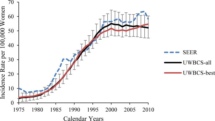
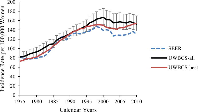
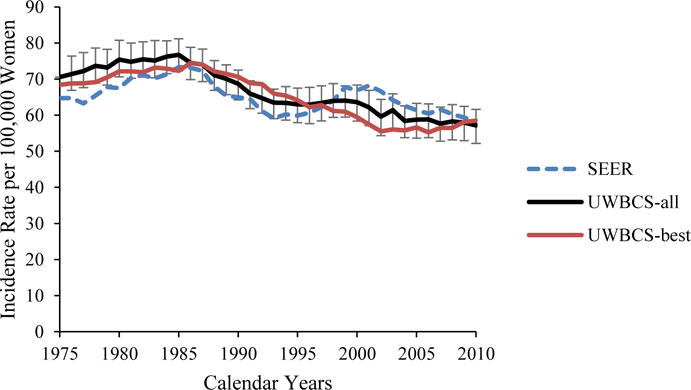
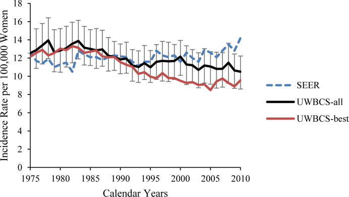
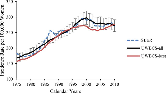
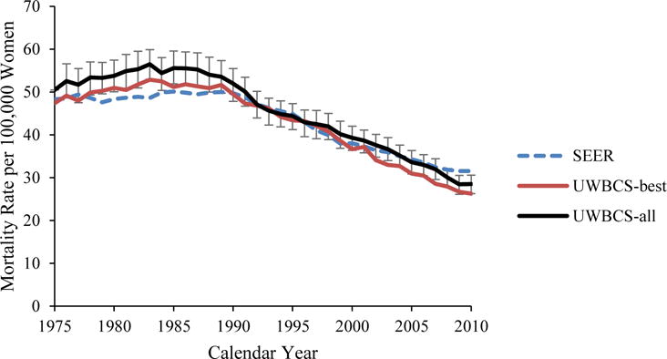
UWBCS-best represents the outcomes obtained when the best input vector is used and UWBCS-all represents the outcomes obtained when 310 input vectors that have a score of 9 or less are used. The errors bars around UWBCS-all represent 95% “uncertainty intervals,” which are generated using the 2.5th and 97.5th percentiles’ values among 310 vectors at each annual time point for each model output.

(a) Age-Adjusted (30–79 years) Insitu Breast Cancer Incidence

(b) Age-Adjusted (30–79 years) Localized Breast Cancer Incidence

(c) Age-Adjusted (30–79 years) Regional Breast Cancer Incidence

(d) Age-Adjusted (30–79 years) Distant Breast Cancer Incidence

(e) Overall Age-Adjusted (30–79 years) Breast Cancer Incidence

(f) Age-Adjusted (30–79 years) Breast Cancer Mortality

Figure 4. Female Breast Cancer Incidence and Mortality over Time in the UWBCS Compared to the Wisconsin Cancer Reporting System (WCRS) and the SEER Program.

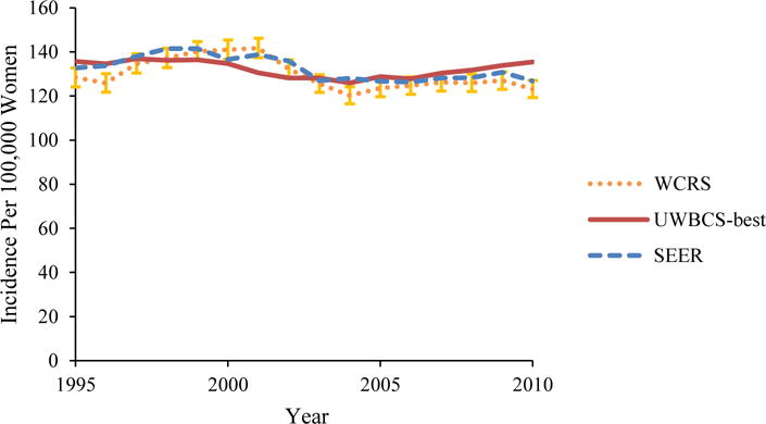
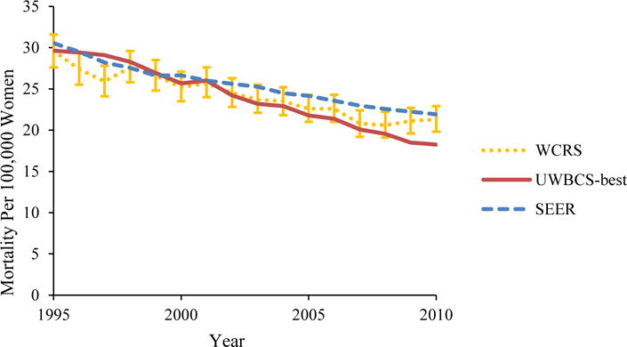
UWBCS-best represents the outcomes obtained when the best input vector is used

(a) Age-Adjusted (all ages) Breast Cancer Incidence

(b) Age-Adjusted (all ages) Breast Cancer Mortality

Figure 5. Survival after Diagnosis Compared to SEER According to Age, Years of Follow-up and Estrogen Receptor (ER) status (1990–1994).

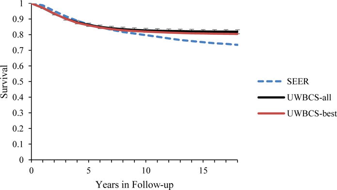
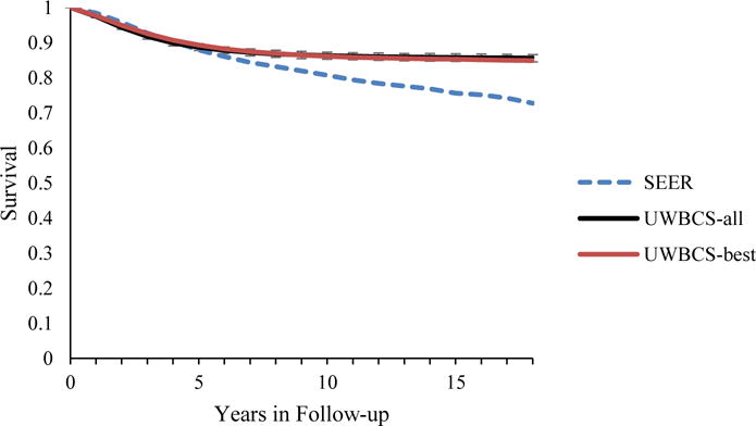
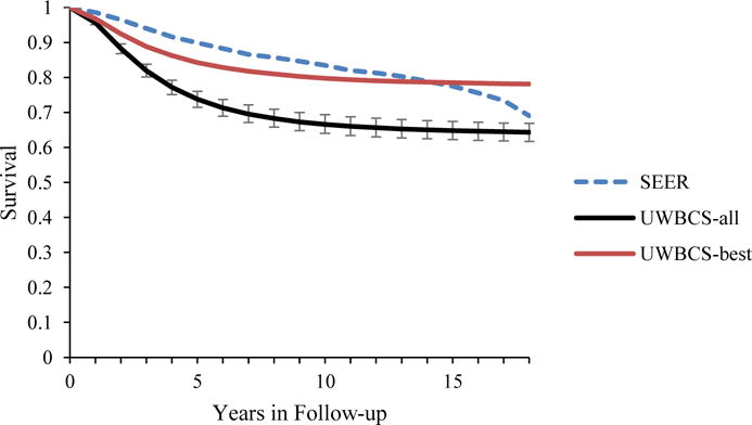
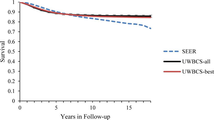
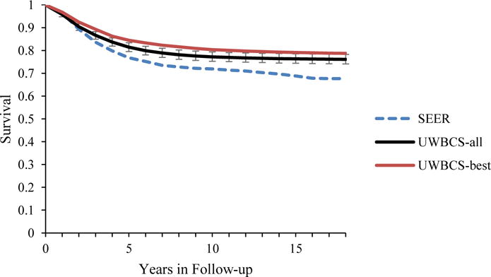
UWBCS-best represents the outcomes obtained when the best input vector is used and UWBCS-all represents the outcomes obtained when 310 input vectors that have a score of 9 or less are used. The errors bars around UWBCS-all represent 95% “uncertainty intervals,” which are generated using the 2.5th and 97.5th percentiles’ values among 310 vectors at each annual time point for each model output. Note that some of the error bars are very narrow therefore are not clearly visible in all of the figures.

(a) All cancers (40–49 years)

(b) All cancers (50–59 years)

(c) All cancers (60–69 years)

(d) All cancers (70–84 years)

(e) ER- cases (50–59 years)

(f) ER- cases (50–59 years)

Recently, we approximated the UK AGE screening trial [28, 29] using U.S.-based data and assuming perfect adherence to invitations for annual screening with 13-year follow-up of women 40–49 and observed that the model projection for mortality reduction closely matched the AGE trial result.[28–30]

7. Conclusions

In summary, the UWBCS has been continuously maintained and updated with new inputs and is able to replicate the observed SEER incidence and mortality between 1975 and 2010. Our model can be used to investigate questions related to breast cancer screening policies such as when to start and end screening and how often to screen. The model can also be used to guide randomized clinical trials that are conducted to test new breast cancer treatment regimens; redesign diagnostic processes in mammography practices, and develop decision aids for individualized mammography screening. The base model has also been expanded to incorporate risk factors and race, and that these expansions enable the model to answer more questions related to breast cancer screening and control. Future work using the UWBCS will take advantage of the recent modeling updates to continue to conduct comparative effectiveness research concerning new interventions to prevent, detect, and treat breast cancer.

References

- 1.Berry DA, Cronin KA, Plevritis SK, Fryback DG, Clarke L, Zelen M, et al. Effect of screening and adjuvant therapy on mortality from breast cancer. New England Journal of Medicine. 2005;353(17):1784–92. doi: 10.1056/NEJMoa050518. [DOI] [PubMed] [Google Scholar]
- 2.Fryback DG, Stout NK, Rosenberg MA, Trentham-Dietz A, Kuruchittham V, Remington PL. The Wisconsin breast cancer epidemiology simulation model. Journal of the National Cancer Institute Monographs. 2006;36:37. doi: 10.1093/jncimonographs/lgj007. [DOI] [PubMed] [Google Scholar]
- 3.Cancer Intervention and Surveillance Modeling Network (CISNET) Breast Cancer Model Profiles. 2016 Jun 27; Available from http://cisnetcancergov/breast/profileshtml 2016.
- 4.Kelton WD, Law AM. Simulation modeling and analysis. McGraw Hill; Boston: 2000. [Google Scholar]
- 5.Holford TR, Cronin KA, Mariotto AB, Feuer EJ. Changing patterns in breast cancer incidence trends. Journal of the National Cancer Institute Monographs. 2005;(36):19–25. doi: 10.1093/jncimonographs/lgj016. [DOI] [PubMed] [Google Scholar]
- 6.Gangnon RE, Sprague BL, Stout NK, Alagoz O, Weedon-Fekjær H, Holford TR, et al. The Contribution of Mammography Screening to Breast Cancer Incidence Trends in the United States: An Updated Age-period-cohort Model. Cancer Epidemiology, Biomarkers & Prevention. 2015 doi: 10.1158/1055-9965.EPI-14-1286. cebp. 12862014. [DOI] [PMC free article] [PubMed] [Google Scholar]
- 7.Shwartz M. Validation and use of a mathematical model to estimate the benefits of screening younger women for breast cancer. Cancer Detection and Prevention. 1980;4(1–4):595–601. [PubMed] [Google Scholar]
- 8.Spratt JS, Spratt JA. Growth rates. Cancer of the Breast. 2002;5:443–76. [Google Scholar]
- 9.Segnan N, Minozzi S, Armaroli P, Cinquini M, Bellisario C, González-Lorenzo M, et al. Epidemiologic evidence of slow growing, nonprogressive or regressive breast cancer: A systematic review. International Journal of Cancer. 2016;139(3):554–73. doi: 10.1002/ijc.30105. [DOI] [PubMed] [Google Scholar]
- 10.Harris JR, Lippman ME, Veronesi U, Willett W. Breast cancer (2) The New England Journal of Medicine. 1992;327(6):390–8. doi: 10.1056/NEJM199208063270606. [DOI] [PubMed] [Google Scholar]
- 11.Harris J, Lippman M, Veronesi U, Willett W. Breast cancer. The New England Journal of Medicine. 1992;327(5):319–28. doi: 10.1056/NEJM199207303270505. [DOI] [PubMed] [Google Scholar]
- 12.Harris JR, Lippman ME, Veronesi U, Willett W. Breast cancer (3) The New England Journal of Medicine. 1992;327(7):473–80. doi: 10.1056/NEJM199208133270706. [DOI] [PubMed] [Google Scholar]
- 13.Zahl P-H, Andersen JM, Mæhlen J. Spontaneous regression of cancerous tumors detected by mammography screening. JAMA. 2004;292(21):2579–80. doi: 10.1001/jama.292.21.2579. [DOI] [PubMed] [Google Scholar]
- 14.Mandelblatt JS, Near AM, Miglioretti DL, Munoz D, Sprague BL, Trentham-Dietz A, et al. Common Model Inputs in Collaborative Breast Cancer Modeling. Medical Decision Making. 2016 doi: 10.1177/0272989X17700624. Submitted. [DOI] [PMC free article] [PubMed] [Google Scholar]
- 15.Jackson H, Vanness D, Stout NK, Alagoz O, Sprague BL, Gangnon RE, et al. Contribution of Breast Cancer to Overall Mortality for U.S. Women by Age, Cohort, Race and Body Mass Index. Medical Decision Making. 2016 Submitted. [Google Scholar]
- 16.Tosteson AN, Stout NK, Fryback DG, Acharyya S, Herman BA, Hannah LG, et al. Cost-effectiveness of digital mammography breast cancer screening. Annals of Internal Medicine. 2008;148(1):1–10. doi: 10.7326/0003-4819-148-1-200801010-00002. [DOI] [PMC free article] [PubMed] [Google Scholar]
- 17.Stout NK, Rosenberg MA, Trentham-Dietz A, Smith MA, Robinson SM, Fryback DG. Retrospective cost-effectiveness analysis of screening mammography. Journal of the National Cancer Institute. 2006;98(11):774–82. doi: 10.1093/jnci/djj210. [DOI] [PubMed] [Google Scholar]
- 18.Lee CI, Cevik M, Alagoz O, Sprague BL, Tosteson AN, Miglioretti DL, et al. Comparative effectiveness of combined digital mammography and tomosynthesis screening for women with dense breasts. Radiology. 2014 doi: 10.1148/radiol.14141237. [DOI] [PMC free article] [PubMed] [Google Scholar]
- 19.Stout NK, Lee SJ, Schechter CB, Kerlikowske K, Alagoz O, Berry D, et al. Benefits, harms, and costs for breast cancer screening after US implementation of digital mammography. Journal of the National Cancer Institute. 2014;106(6):dju092. doi: 10.1093/jnci/dju092. [DOI] [PMC free article] [PubMed] [Google Scholar]
- 20.Sprague BL, Stout NK, Schechter C, van Ravesteyn NT, Cevik M, Alagoz O, et al. Benefits, harms, and cost-effectiveness of supplemental ultrasonography screening for women with dense breasts. Annals of Internal Medicine. 2015;162(3):157–66. doi: 10.7326/M14-0692. [DOI] [PMC free article] [PubMed] [Google Scholar]
- 21.Nelson HD, Zakher B, Cantor A, Fu R, Griffin J, O’Meara ES, et al. Risk factors for breast cancer for women aged 40 to 49 years: a systematic review and meta-analysis. Annals of internal medicine. 2012;156(9):635–48. doi: 10.1059/0003-4819-156-9-201205010-00006. [DOI] [PMC free article] [PubMed] [Google Scholar]
- 22.Carney PA, Miglioretti DL, Yankaskas BC, Kerlikowske K, Rosenberg R, Rutter CM, et al. Individual and combined effects of age, breast density, and hormone replacement therapy use on the accuracy of screening mammography. Annals of internal medicine. 2003;138(3):168–75. doi: 10.7326/0003-4819-138-3-200302040-00008. [DOI] [PubMed] [Google Scholar]
- 23.Batina NG, Trentham-Dietz A, Gangnon RE, Sprague BL, Rosenberg MA, Stout NK, et al. Variation in tumor natural history contributes to racial disparities in breast cancer stage at diagnosis. Breast Cancer Research and Treatment. 2013;138(2):519–28. doi: 10.1007/s10549-013-2435-z. [DOI] [PMC free article] [PubMed] [Google Scholar]
- 24.Cevik M, Ergun MA, Stout NK, Trentham-Dietz A, Craven M, Alagoz O. Using Active Learning for Speeding up Calibration in Simulation Models. Medical Decision Making. 2015:0272989X15611359. doi: 10.1177/0272989X15611359. [DOI] [PMC free article] [PubMed] [Google Scholar]
- 25.Alagoz O, Berry D, Feuer EJ, de Koning H, Lee SJ, Plevritis S, et al. Introduction to the Cancer Intervention and Surveillance Modeling Network (CISNET) Breast Working Group (BWG) Models. Medical Decision Making. 2016 doi: 10.1177/0272989X17737507. Submitted. [DOI] [PMC free article] [PubMed] [Google Scholar]
- 26.van den Broek JJ, van Ravesteyn NT, Cevik M, Schechter CB, Lee SJ, Munoz D, et al. Comparison of model structure across CISNET breast cancer simulation models using MCLIR methodology. Medical Decision Making. 2016 doi: 10.1177/0272989X17743244. Submitted. [DOI] [PMC free article] [PubMed] [Google Scholar]
- 27.van Ravesteyn NT, van den Broek JJ, Li X, Weedon-Fekjar H, Schechter CB, Alagoz O, et al. Modeling ductal carcinoma in situ (DCIS) – an overview of CISNET model approaches. Medical Decision Making. 2016 doi: 10.1177/0272989X17729358. Submitted. [DOI] [PMC free article] [PubMed] [Google Scholar]
- 28.Moss SM, Cuckle H, Evans A, Johns L, Waller M, Bobrow L. Effect of mammographic screening from age 40 years on breast cancer mortality at 10 years’ follow-up: a randomised controlled trial. The Lancet. 2006;368(9552):2053–60. doi: 10.1016/S0140-6736(06)69834-6. [DOI] [PubMed] [Google Scholar]
- 29.Moss SM, Wale C, Smith R, Evans A, Cuckle H, Duffy SW. Effect of mammographic screening from age 40 years on breast cancer mortality in the UK Age trial at 17 years’ follow-up: a randomised controlled trial. The Lancet Oncology. 2015 doi: 10.1016/S1470-2045(15)00128-X. [DOI] [PubMed] [Google Scholar]
- 30.Mandelblatt JS, Cronin K, de Koning H, Miglioretti DL, Schechter C, Stout NK. Modeling Report: Collaborative Modeling of U.S. Breast Cancer Screening Strategies: Breast Cancer: Screening. U.S. Preventive Services Task Force; 2015. [cited September 12, 2015 Available from: http://www.uspreventiveservicestaskforce.org/Page/Document/modeling-report-collaborative-modeling-of-us-breast-cancer-1/breast-cancer-screening1. [Google Scholar]
- 31.Munoz D, Near AM, van Ravesteyn NT, Lee SJ, Schechter CB, Alagoz O, et al. Effects of Screening and Systemic Adjuvant Therapy on ER-Specific US Breast Cancer Mortality. Journal of the National Cancer Institute. 2014;106(11):dju289. doi: 10.1093/jnci/dju289. [DOI] [PMC free article] [PubMed] [Google Scholar]
- 32.Centers for Disease Control and Prevention. National Health and Nutrition Examination Survey. 2016 Available from http://www.cdc.gov/nchs/nhanes/]
- 33.Shiyanbola OO, Arao RF, Miglioretti DL, Sprague BL, Hampton JM, Stout NK, et al. Emerging Trends in Family History of Breast Cancer and Associated Risk. 2017 doi: 10.1158/1055-9965.EPI-17-0531. Submitted. [DOI] [PMC free article] [PubMed] [Google Scholar]
- 34.Trentham-Dietz A, Sprague BL, Hampton JM, Miglioretti DL, Nelson HD, Titus LJ, et al. Modification of breast cancer risk according to age and menopausal status: a combined analysis of five population-based case–control studies. Breast Cancer Research and Treatment. 2014;145(1):165–75. doi: 10.1007/s10549-014-2905-y. [DOI] [PMC free article] [PubMed] [Google Scholar]
- 35.Centers for Disease Control and Prevention. National Health Interview Survey. 2016 Available from http://www.cdc.gov/nchs/nhis/]
- 36.Munsell MF, Sprague BL, Berry DA, Chisholm G, Trentham-Dietz A. Body mass index and breast cancer risk according to postmenopausal estrogen-progestin use and hormone receptor status. Epidemiologic Reviews. 2014;36(1):114–36. doi: 10.1093/epirev/mxt010. [DOI] [PMC free article] [PubMed] [Google Scholar]
- 37.American College of Radiology BI-RADS Committee. ACR BI-RADS Atlas: Breast Imaging Reporting and Data System. 2013 [Google Scholar]
- 38.Breast Cancer Surveillance Consortium. Breast Cancer Surveillance Consortium. 2016 Available from http://www.bcsc-research.org/]
- 39.Sprague BL, Gangnon RE, Burt V, Trentham-Dietz A, Hampton JM, Wellman RD, et al. Prevalence of mammographically dense breasts in the United States. Journal of the National Cancer Institute. 2014;106(10):dju255. doi: 10.1093/jnci/dju255. [DOI] [PMC free article] [PubMed] [Google Scholar]
- 40.Jewett PI, Gangnon RE, Trentham-Dietz A, Sprague BL. Trends of postmenopausal estrogen plus progestin prevalence in the United States between 1970 and 2010. Obstetrics and gynecology. 2014;124(4):727–33. doi: 10.1097/AOG.0000000000000469. [DOI] [PMC free article] [PubMed] [Google Scholar]
- 41.Sprague BL, Trentham-Dietz A, Cronin KA. A sustained decline in postmenopausal hormone use: results from the National Health and Nutrition Examination Survey, 1999–2010. Obstetrics and gynecology. 2012;120(3):595. doi: 10.1097/AOG.0b013e318265df42. [DOI] [PMC free article] [PubMed] [Google Scholar]
- 42.Centers for Disease Control and Prevention. Behavioral Risk Factor Surveillance System. 2016 Available from http://www.cdc.gov/brfss/]
- 43.Cronin KA, Miglioretti DL, Krapcho M, Yu B, Geller BM, Carney PA, et al. Bias associated with self-report of prior screening mammography. Cancer Epidemiology, Biomarkers & Prevention. 2009;18(6):1699–705. doi: 10.1158/1055-9965.EPI-09-0020. [DOI] [PMC free article] [PubMed] [Google Scholar]