Adding experimental arms to platform clinical trials: randomization procedures and interim analyses

SUMMARY

Multi-arm clinical trials use a single control arm to evaluate multiple experimental treatments. In most cases this feature makes multi-arm studies considerably more efficient than two-arm studies. A bottleneck for implementation of a multi-arm trial is the requirement that all experimental treatments have to be available at the enrollment of the first patient. New drugs are rarely at the same stage of development. These limitations motivate our study of statistical methods for adding new experimental arms after a clinical trial has started enrolling patients. We consider both balanced and outcome-adaptive randomization methods for experimental designs that allow investigators to add new arms, discuss their application in a tuberculosis trial, and evaluate the proposed designs using a set of realistic simulation scenarios. Our comparisons include two-arm studies, multi-arm studies, and the proposed class of designs in which new experimental arms are added to the trial at different time points.

1. Introduction

Multi-arm studies that test several experimental treatments against a standard of care are substantially more efficient compared to separate two-arm studies, one study for each experimental treatment. Multi-arm studies test experimental treatments against a common control arm, whereas when experimental drugs are evaluated using two-arm studies the control arm is replicated in each study. This difference reduces the overall sample size for testing multiple experimental drugs in a single multi-arm study compared to using independents two-arm trials. The gain in efficiency is substantial and has been discussed by various authors (Freidlin and others, 2008; Wason and others, 2014).

The use of response-adaptive assignment algorithms can further strengthen the efficiency gain of multi-arm studies compared to two-arm studies (Berry and others, 2010; Trippa and others, 2012; Wason and Trippa, 2014; Ventz and others, 2017). As the trial progresses, adaptive algorithms typically increase randomization probabilities towards the most promising treatments. On average, this translates into larger sample sizes for the arms with positive treatment effects and, in turn, into higher power of detecting the best treatments at completion of the study.

Multi-arm studies also reduce fixed costs compared to two-arm trials. Designing and planning a study is a time-consuming and costly process, which involves clinicians and investigators from different fields. Compared to independent two-arm studies, multi-arm trials have the potential to reduce the resources needed to evaluate experimental drugs. Based on these arguments, regulatory agencies encourage the use of multi-arm studies (FDA, 2013; Freidlin and others, 2008).

Nonetheless, multi-arm studies constitute a small fraction of the ongoing early stage clinical studies. A major bottleneck in their implementation is the requirement that all therapies, often drugs from different pharmaceutical companies, must to be available for testing when the clinical trial starts. Experimental drugs are rarely at the same stage of development. During the design period, before the study starts, there are several candidate drugs with promising preclinical or clinical data. But often some of these drugs are not available when the trial starts recruiting patients due to logistical reasons, investigators’ concerns, or because the pharmaceutical company decides to wait for results from other studies (e.g. from a clinical trial for a different disease). Additionally, holdups in the supply chain are not uncommon. Investigators thus face a choice between delaying the start of the trial or testing only a subset of drugs.

Here we consider the design of multi-arm trials wherein new experimental treatments are added at one or multiple time points. Our work is motivated by the endTB trial, a Bayesian response-adaptive Phase III study in tuberculosis that we designed (Cellamare and others, 2017). The study originally sought to evaluate eight experimental treatments. While designing the trial, it became clear that four drugs would have not been available for the initial 12 months of the study or longer. Because of the need to test an increasing number of experimental treatments (Berry and others, 2015) similar examples exist in several other disease areas. Recent cancer studies (STAMPEDE, AML15, and AML16), the neurology trial NET-PD, and the schizophrenia study CATIE, to name a few, added or considered adding experimental drugs to ongoing studies (Hills and Burnett, 2011; Lieberman and others, 2005; Burnett and others, 2013; Elm and others, 2012). Similarly, the pioneering breast cancer trial I-SPY2 (Barker and others, 2009) adds and removes arms within a Bayesian randomized trial design.

Nonetheless, statistical studies of designs that allows the addition of arms to an ongoing trial are limited. A recent literature review of designs that involved the addition of experimental arms Cohen and others (2015) concluded that the statistical approaches remain mostly ad hoc: few guidelines are available for controlling and optimizing the operating characteristics of such studies, and the criteria for evaluating the designs remain unclear. Recent contributions that consider the amendment of one additional arm into an ongoing study and platform designs include Elm and others (2012), Hobbs and others (2016), and Yuan and others (2016).

We focus on randomization procedures and inference for trials during which new experimental arms are added. We discuss three randomization methods and study their operating characteristics. The first one is a balanced randomization (BR) algorithm. In this case the arm-specific accrual rates vary with the number of treatments available during the trial. We show that the approach yields substantial efficiency gains compared to separate two-arm studies. The other two methods use the outcome data to adaptively vary the randomization probabilities. One of the algorithms has close similarities with Bayesian adaptive randomization (BAR) (Thall and Wathen, 2007; Lee and others, 2010), while the other shares similarities with the doubly adaptive biased coin design (DBCD) (Eisele, 1994). In all three cases the relevant difference between the designs that we consider and BR, BAR, or DBCD is the possibility of adding new experimental arms to an ongoing trial. We also introduce a Bootstrap procedure to test efficacy under the proposed platform designs. The algorithm extends previously introduced bootstrap schemes (Rosenberger and Hu, 1999; Trippa and others, 2012) to platform trial designs with group-sequential interim analysis (IA). The resampling method estimates sequentially stopping boundaries that correspond to pre-specified type-I error values at interim and final analyses.

We describe in Sections 2.1, 2.2, and 2.3 the three designs for balanced and outcome-adaptive multi-arm trials, during which experimental arms can be added. In Section 3, these randomization procedures are combined with early stopping rules and a bootstrap algorithm for testing efficacy. Section 4 evaluates the proposed designs in a simulation study. In Section 5, we compare the performances of the three designs under scenarios tailored to the endTB trial. Section 6 concludes the article with a discussion.

2. Adding arms to an ongoing trial

We consider a clinical trial that initially randomizes patients to either the control arm or to experimental arms. For each patient , indicates that patient has been randomized to arm , where is the control arm. In what follows, counts the number of patients randomized to arm before the -th patient, while is the number of observed outcomes for arm before the -th enrollment. Different values of and are typically due to a necessary period, after randomization and before the patients’ outcome can be measured. We consider binary outcomes. The random variable counts the number of observed positive outcomes, and has a binomial distribution with size and response probability . The available data at the -th enrollment is denoted by . The goal is to test treatment efficacy, with null hypotheses , one null hypothesis for each experimental arm.

We consider a design where experimental arms are added at different time points. At the arrival of the -th patient, , experimental arms are added to the trial, and the sample size of the study is increased by additional patients, so that the final sample size becomes . In most cases and only one or two arms are added. We do not assume that the number of adding times , or the number of added arms , are known in advance, when the study is designed. Thus, we treat and as random variables.

2.1 Balanced randomization

A non-adaptive randomization algorithm for a multi-arm trial assigns patients to control and experimental arms with a ratio . Here are pre-specified non-negative weights, for instance , that determine the ratio of patients assigned to the control arm compared to each experimental arm.

The overall sample size is , where the number of patients treated with the control arm and each experimental arm are selected based on targeted type I/II error probabilities. For the moment, we do not consider early stopping.

Here we describe a randomization scheme for adding new treatments, focusing on the case of first. We define the indicator , which is one if and zero otherwise. The first patients are randomized to the control arm or the initial experimental arms with probabilities proportional to and . At the arrival of the -th patient, arms are added, and the sample size is extended by patients, for the control arm and for each added arm. The remaining patients are then randomized to the initial arms or to the added arms , with probabilities

(2.1)

where At the completion of the study, patients have been assigned to each experimental arm , and patients are assigned to the control arm. In early phase trials, one can potentially set and use the control data from patients randomized before and after the -th enrollment, to evaluate the added experimental arms. An additional patients for the control arm may be necessary for longer studies with a slow accrual and potential drifts in the population. The parameter modulates the enrollment rate to the new arms after these arms have been added to the trial. The choice of should depend on . For example, with equal to , and , all arms complete accrual at approximately the same time (see Figure 1).

Fig. 1.

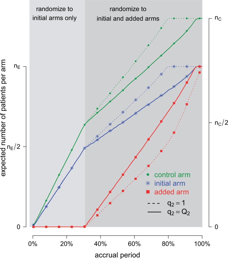
Adding experimental arms to a multi-arm BR trial. We consider a trial with two initial arms and two added experimental arms. The graph shows the expected number of patients randomized to an arm during the accrual period for the control , one initial arm in and one added arm in . The two additional arms were added after 50% of the initially planned sample size, at . Patients were initially randomized to the control or experimental arm with ratio to . Dashed lines correspond to . Solid lines correspond to the , in this case all arms are expected to complete accrual at the same time. Bold numbers are operating characteristics of effective experimental arms.

The case is similar. At the enrollment of the -th patient (), new arms are added; and the sample size is increased by patients, patients for the control, and for the new arms. Let be the -th group of treatments, where is the set of initial experimental arms and . Patient is assigned to an active arm , with probability

(2.2)

As before, the parameters , control how quickly each group of arms enrolls patients compared to the previously added arms. For example, with and equal to

(2.3)

for , all arms complete accrual at approximately the same time.

The step function leads to a randomization scheme, where the assignment of the last patient(s) enrolled in the trial can be predicted. Alternatively one can replace the indicator by a smoothly decreasing function.

Example 2.1

We consider a multi-arm trial with experimental arms and a control arm with response probability of after 8 weeks of treatment. A multi-arm trial with and targeted type I/II error probabilities of 0.1 and 0.2 requires an overall sample size of patients to detect treatment effects of , with patients. With an accrual rate of six patients per month, the trial duration is approximately months. We can now introduce a departure from this setting. Two treatments become available approximately and months after the beginning of the trial (, and ). We describe three designs. (1) The first one uses all outcomes of the control arm available at completion of the study to evaluate arms . In this case, and for with definition of as in (2.3). (2) To avoid bias from possible population trends, the second design estimates treatment effects of arm using only control outcomes of patients randomized to the control arm after the -th enrollment. In this case, to maintain a power of 80% for the added arms, and to keep the accrual ratios constant during the active accrual period of each treatment , we set and at the -th and -th arrival. (3) We also consider a third strategy with three independent trials; one for the initial experimental arms, and two additional two-arm trials for arm and , each study has its own control arm. We assume again an average enrollment of 6 patients per month. Design 1 requires 265 patients, and the treatment effect estimates are available approximately 45 months after the first enrollment. Design 2, with , requires on average patients. Treatment effects estimates are available approximately 37, 47, and 53 months after the first enrollment. The three independent trials in design 3 would instead require patients and the effect estimates are available approximately 46, 60, and 64 months after the first patient is randomized.

2.2 Bayesian adaptive randomization

BAR uses accumulating data during the trial to vary the randomization probabilities (Thall and Wathen, 2007; Lee and others, 2010). Initially, BAR randomizes patients with equal probabilities to each arm. As the trial progresses and information on efficacy becomes available, randomization favors the most promising treatments. This can translate into a higher power compared to balanced designs (Wason and Trippa, 2014).

We complete the outcome model with a prior for the response probabilities of arm . We use a conjugate beta distributions with parameters . To predict the response probabilities of new arms in the group , even when no outcome data are available for treatments in , we leverage on hierarchical modeling with a hyper-prior . We use a discrete uniform distribution over a grid of possible values.

When we do not add arms, , BAR assigns patient to arm with probability

(2.4)

where , and the function is increasing in the number of enrolled patients (Thall and Wathen, 2007). Initially equals zero, and randomization is balanced. As more information becomes available, increases and more patients are randomized to the most promising arms. The randomization probability of the control arm in (2.4) is defined to approximately match the sample size of the control and the most promising treatment. This characteristic preserves the power of the adaptive design (Trippa and others, 2012).

We extend BAR to allow the addition of new arms. We first consider . At the -th arrival, new arms are added and the sample size is increased by patients. The randomization probabilities are defined as

(2.5)

where and . We introduce group-specific scaling and power functions and . The power function controls the exploration–exploitation trade-off within each group . The scaling function has two purposes: (i) It introduces an initial exploration advantage for newly added treatments, which compete for accrual with all open arms. (ii) It ensures sufficient exploration of all treatment groups . Several functions serve both purposes. We use a Gompertz function

(2.6)

where is the number of patients randomized to the group of experimental arms and are tuning parameters. The function has an initial plateau at , followed by a subsequent lower plateau at . The initial plateau provides group with a necessary exploration advantage when the number of patients randomized to group is small, i.e. . During the later stage of the trial, once a sufficient number of patients has been assigned to treatments in group , i.e. , the scaling function reaches the lower plateau, and patients are assigned to treatment arms approximately according to standard BAR.

We noted that limiting the maximum number of patients per arm can avoid extremely unbalanced allocations. This may be achieved, for example, by multiplying the Gompertz function in (2.6) by the indicator , where represents a desired maximum number of patients in each experimental arm.

We use a function that is increasing in the number of patients randomized to arms in with a maximum after enrollments. Similarly, for the added arms in , is increasing in the number of patients randomized to , with a maximum at . In particular is equal to if and otherwise, where and, as explained above, denotes the extension of the overall sample size after enrollments.

The general case is similar. Each patient is randomized to the available treatments with probabilities

(2.7)

where and are defined as in (2.5), and is the Gompertz function defined in (2.6). For the scheme reduces to standard BAR. The parameter of the scaling function can be selected at the -th arrival such that the expected number of patients assigned to each arm in under a selected scenario equals a fixed predefined value.

Example 2.2

We consider the same trial as in Example 2.1, but use a BAR design instead. To simplify comparison to BR, we set the overall sample size to as for BR. We can easily verify that if and , the BAR and BR designs (with ) are identical. We now describe the major operating characteristics under three scenarios. In scenarios 1 to 3, either arm , or arm added at , or arm added at have positive treatment effects, . In each scenario, the remaining 4 of the 5 arms, including the control, have identical response rates equal to 0.3. We tuned the parameters of the design to maximize power under the assumption that there is a single effective arm and , . The tuning parameter for the Gompertz function and are selected through simulations, to get approximately the same average sample size for each arm when for all arms.

As for BR, in all three scenarios, the trial completes accrual after approximately 45 months. In scenario 1, BAR randomizes on average 64 patients to arm and to the control arm across 5000 simulations, while on average (43, 46, 47) patients are assigned to the ineffective arms 2, 3, 4 with standard deviations (SDs) of 4.7, 6.4, 7.4, 5.3, and 5.4 (see Table 1). The power increases to 85%—compared to 80% for BR—with an identical overall sample size. In scenarios 2 and 3, BAR randomizes on average 64 and 63 patients to arm and , respectively. This translates into 86% and 85% power for the added arms 3 and 4, respectively, compared to 80% for BR.

Table 1.

Expected sample size (E), standard deviation (SD) and power (Po) for experimental arm 1, the first added arm and the second added arm for a trial with two initial experimental arms, and two arms which are added after 12 and 24 month,

Scenario	Control		Arm 1			First added arm			Second added arm
	E	SD	E	SD	Po	E	SD	Po	E	SD	Po
BR 1	53	0.0	53	0.0	0.11	53	0.0	0.10	53	0.0	0.10
2	53	0.0	53	0.0	0.80	53	0.0	0.11	53	0.0	0.11
3	53	0.0	53	0.0	0.11	53	0.0	0.80	53	0.0	0.10
4	53	0.0	53	0.0	0.11	53	0.0	0.11	53	0.0	0.80
BAR 1	62	3.7	50	10.1	0.10	51	7.6	0.10	52	6.9	0.10
2	64	4.7	64	6.4	0.85	46	5.3	0.11	47	5.4	0.10
3	64	4.3	45	7.8	0.10	64	5.8	0.86	47	5.7	0.11
4	62	3.4	46	8.2	0.10	48	5.9	0.11	62	5.5	0.85
DBCD 1	57	3.3	52	4.8	0.10	52	4.6	0.10	52	4.3	0.10
2	60	3.9	59	4.0	0.82	48	4.4	0.10	49	4.2	0.10
3	58	3.6	49	4.6	0.10	59	3.8	0.82	48	4.1	0.10
4	58	3.4	50	4.5	0.09	49	4.3	0.10	58	3.4	0.83

Results are based on 5000 simulated trials under balanced randomization (BR), Bayesian adaptive randomization (BAR) and a doubly adaptive biased coin design (DBCD) without early stopping rules. The initial planned overall sample size is , which is then extended by patients for each added arm. Bold numbers are operating characteristics of effective experimental arms.

2.3 Doubly adaptive biased coin design

The DBCD (Eisele, 1994) is a response adaptive randomization scheme that seeks to assign patients to treatments according to a vector of target proportions that depends on response rates. Examples include the Neyman allocation and (Hu and Zhang, 2004). Since the response probabilities are unknown, the target allocation is estimated from the accumulated data by . For , patients are randomized to arm with probabilities

(2.8)

Here, varies with the ratio of (i) the estimated target allocation proportion and (ii) the current number of patients that are randomized to arm (Hu and Zhang, 2004). If the current proportion of patients assigned to arm is smaller than the target, then for the next patient, the randomization probability to arm will be larger than and vice versa. Larger values of yield stronger corrections towards the target. As for BAR, we limit the maximum number of patients per arm by multiplying the correction by the indicator .

We now consider adding new experimental arms during the study. Until the -th arriving patient, the target is a function of , and it is estimated through the hierarchical Bayesian model in Section 2.2 by . Patient is randomized to the control or experimental arm with probabilities defined by (2.8). Then, at the enrollment of the -th patient, , arms are added, and the overall sample size is increased by patients. Before observing any outcome for arm , the target is re-defined to , with . The posterior distribution of the hierarchical model is used to compute for all initial and added arms . Also in this case, the function is used to approximately match the patient allocation to arm with the estimated target . Each patient is randomized to the control arm or to treatments for groups added before the -th arrival with probability

(2.9)

For treatments in , the functions correct the current allocation proportions towards the estimated target.

To avoid extremely unbalanced randomization probabilities, we can replace in expression (2.9) with , where is a function of the data . We used , a decreasing function of the number of active arms. Also for the DBCD design, the function increases during time with if and otherwise. The interpretations of the functions in the DBCD and BAR designs are different, and in our simulation studies the parameters are tuned separately for these trial designs.

Example 2.3

We consider again the setting in Examples 2.1 and 2.2, and use a DBCD design for the trial. Following Hu and Zhang (2004) we use the target allocation for . To preserve the power of the design, similarly to Example 2.2, we use to approximately match the sample size of the control and the most promising experimental arm. For comparison to Examples 2.1 and 2.2 we use again an overall sample size of and . If the response probabilities for all arms are , a DBCD with and randomizes on average patients to each experimental arm, and 57 to the control (SD 3.3, 4.8, 4.8, 4.6, and 4.3). We consider the same scenarios as in Examples 2.1 and 2.2.

In all 3 scenarios, the trial closes after approximately 45 months, as for BR and BAR. In scenario 1, DBCD randomizes on average 59 and 60 patients to arm 1 and the control (the target is 61), and approximately patients to the remaining ineffective arms (SD 3.9, 4.0, 4.6, 4.4, and 4.2). The power is 82% for arm , while it is 80% and 85% under BR and BAR in Examples 2.1 and 2.2, respectively. For scenarios 2 and 3, the DBCD randomizes on average 59 and 58 patients to the effective arms and (SD of 3.8 and 3.4). Compared to 80% and 85% for BR and BAR the power of the DBCD becomes 82%. Similarly in scenario 3, for arm 4 we have a power equal to 82% using the DBCD compared to 80% and 85% using BR and BAR.

3. Early stopping rules and hypothesis testing

We describe hypothesis testing and early stopping rules. We consider the interpretable strategy where arm in group is stopped for futility after the enrollment of the -th patient if the posterior probability of a treatment effect, falls below the boundary , i.e. . Here increases from to when the number of observed outcomes for arm is equal to the maximum accrual , for BR .

3.1 A bootstrap test for platform trials without early stopping for efficacy

For a platform trial , if arm added after enrollments is not stopped for futility, we compute a bootstrap P-value estimate at a pre-specified time , for example when reaches , or at the completion of the trial . The bootstrap procedure is similar to the algorithms discussed in Rosenberger and Hu (1999) and in Trippa and others (2012). We use the statistic , the standardized difference between the estimated response rate of arm and the control, to test the null hypothesis at significance level . Large values of indicate evidence of a treatment effect. The algorithm estimates the distribution of under the null hypothesis and the platform design, which includes changes of the randomization probabilities when new experimental arms are added.

If the estimated response probability for experimental arm is smaller than the estimated probability for the control , we don’t reject the null hypothesis . If , we use the following bootstrap procedure, which is also summarized in Algorithm 1:

• (i) For all arms that enrolled patients before time , we compute maximum likelihood estimates (MLEs) . For arm and the control, we restrict the MLE to .

• (ii) The algorithm then simulates trials , from the first enrollment until time . Here is defined identical to and corresponds to simulation . In each simulation , arms are added to the study after enrollments, for all , and randomization probabilities are updated as described in Section 2. Patients in these simulations respond to treatments with probabilities and the simulations’ accrual rate is identical to the accrual rate of the actual trial .

• (iii) For each simulation we compute the test statistics at time , and set equal to zero if arm was stopped early for futility and equal to one otherwise. The simulations generate test statistics under the null hypothesis and the platform design. We can therefore estimate the P-value by and reject at level if .

3.2 A bootstrap test for platform trials with early stopping for efficacy

We extend the procedure described in the previous section and include early stopping for efficacy. In this case, there is a connection between the -spending method of Lan and DeMets (1983) and our algorithm. We consider IA, conducted after a pre-specified set of observed outcomes. At each IA, the arms that are evaluated for efficacy may vary, for instance because arms have been added or removed from the trial. We partition the type I error probability into pre-specified values for each IA . For each initial and added arm , the algorithm estimates the thresholds defined by the following target. Under the platform design and the unknown combination , where we replace with , the probability of stopping arm for efficacy at the IA is Here if arm is stopped before the -th IA and equals 1 otherwise, while is the test statistics computed at IA . In what follows, simulations under the null hypothesis are generated using the estimates . We tested the following algorithm for up to six IA and eight arms:

First IA: We compute the MLEs and the statistics for all initial and added arms that enrolled patients before the first IA. Then, separately for each of these arms :

• (i) We generate platform trials under , from the first enrollment until the first IA. In these simulations, all arms which have been added to the actual trial before the first IA are successively added to the simulated trial , and patients respond to treatment with probability By adding these arms to the trial before the first IA we account for and mimic in simulation the variations of the randomization probabilities after the new arms have been added.

• (ii) We then compute the test statistics and the indicator variable for each simulated trial , with definitions identical to those of for the actual trial . The threshold is then estimated by and arm is stopped for efficacy at the first IA if and .

Second IA: We recompute the MLEs using the data available at the second IA.

• (i) Separately for each arm added before the second IA we re-estimate using a new set of simulations under from the first enrollment until the first IA.

• (ii) In these new simulations , if for any arm that enrolled patients before the first IA the statistics and , then arm is stopped for efficacy in the simulated trial . This part of the algorithm creates, for each arm that enrolled patients before the first IA, simulations under that cover the time window from the first enrollment until the first IA.

• (iii) Simulations then continue beyond the first IA. After the thresholds ’s have been recomputed, we extend, for each arm , the new simulations in time to cover the window between the first and the second IAs. Importantly, these simulations include early stopping at the first IA. Analogous to the first IA, if new arms (e.g. ) are added between the first and second IAs, then, starting from the -th enrollment, all simulations will include the added arms to mimic the actual platform trial.

• (iv) We estimate and then stop arm at the second IA for efficacy if and .

th IA The same procedure is iterated similarly to for all other IAs . In some simulations of the multi-arm study under , where , arm might not appear because the experimental arms have been all dropped and the trial stopped before enrollments. To account for this, all simulations under (when ) are generated conditional on the event that the multi-arm study enrolls more than patients.

We refer to the Supplementary material available at Biostatistics online for an example (Example S1.1) of the described algorithm. We also include in the Supplementary material available at Biostatistics online, a discussion on hypothesis testing and departures from the error rate when the patient population varies during the trial.

4. Simulation study

We continue Examples 2.1, 2.2, and 2.3 using four scenarios. In scenario 1 no experimental arm has a treatment effect. Whereas in scenarios 1–3 either the initial arm , the first added arm , or the second added arm is effective with response rate of 0.5. The remaining experimental arms have response rates equal to the control rate of 0.3. The initial sample size is and , and the type I error is controlled at 10%.

Both, BAR and DBCD, can assign at most patients to each experimental arm, and all three designs use outcomes from patients randomized to the control before and during the accrual period of the added arms to define randomization probabilities and for hypothesis testing. In Section S2 of supplementary available at Biostatistics online, we outline possible modifications of the designs when trends on the patient population during the trial represent a concern.

We used the same parameters to define the randomization probabilities as in Examples 2.1, 2.2, and 2.3. For BR the scaling parameters equal , with defined in (2.3), and . The parameters of the Gompertz function in BAR equal and . For DBCD we used and and the randomization probabilities for active arms have been restricted to values larger than Here if and arm has not been stopped before the enrollment of the -th patient, and the indicator is equal to zero otherwise.

We first summarize the operating characteristics of the three designs without early stopping to illustrate the performance of the randomization schemes. The three designs are compared to three independent trials; one trial for the initial two experimental arms, and two independent two-arm studies for the added arms and , each with their own control arms. We indicate them as balanced randomized and independent trials (BRI). The overall rate of accrual of the three independent trials in BRI is set to six patients per month, and is assumed to be identical for the competing studies.

Figure 2 shows the median number of patients randomized to arms and as a function of the overall number of patients enrolled in the trial. For each scenario and design, the plotted graph represents for a fixed arm the median number of patients assigned to arm over 5000 simulated trials (y-axis), after a total of (371 for BRI) patients have been enrolled to the trial (x-axis). Under BRI, 106 additional patients are necessary for the two additional control arms. This prolongs the trials and slows down the accrual to experimental arms.

Fig. 2.

Number of patients randomized to treatment arms during the accrual period of the study, for a trial with two initial experimental arms and two arms that are added after the enrollment of and patients. BRI corresponds to a design that uses three balanced and independent trials—one trial for the initial arms and one two-arm trial for each added arm, BR, BAR, and DBCD denote balanced randomization, Bayesian adaptive randomization and the doubly adaptive biased coin design. For each arm , the plotted graph represents the median number of patients assigned to arm , after a total of patients have been randomized. In scenario 1 all experimental arms are ineffective, whereas in scenarios 2–4 either arm 1, the first or the second added arm have a treatment effect, with a response probability of 0.5 compared to 0.3 for the control.

Figure S1 of supplementary available at Biostatistics online shows the variability of treatment assignments at the end of the trial. In scenario 1, DBCD has a median accrual of 52 patients for all experimental arms with interquartiles (IQ) for arms 1 and 2, and an IQ of for arms 3 and 4. In comparison, using BAR, the median accrual for the first two experimental arms is 49 (IQ: 42, 58), and for the two added arms the median equals 50 and 52 with IQs of (48, 57) and (45, 56). In scenario 2, where the first initial arm has a positive effect, BAR and DBCD have a median accrual of 66 (IQ: 61,70) and 59 (IQ: 57,62) patients for this arm, with 85% and 82% power, compared to 80% using BR (Table 1). In scenario 3, BAR and DBCD have 86% and 82% power of detecting the effect of the first added arm, respectively, compared to 80% under BR (Table 1). The median accrual for the first added arm is 65 (IQ: 60,69) patients for BAR and 59 (IQ: 57, 62) for DBCD. Lastly, in scenario 4 the second added arm has a positive effect. BAR and DBCD assign a median number of 63 (IQ: 56, 66) and 58 (IQ: 56, 61) patients to this arm, which translates into 85% and 83% power, respectively.

We now compare BR, BAR, and DBCD, when early stopping for efficacy and futility are included as described in Section 3. The tuning parameters of the futility stopping boundaries is selected such that the probability of stopping an effective initial arm early for futility is approximately 1%, for BR, and for BAR and DBCD. Larger values of (1 to 2.5) decrease the probability of dropping an arm for futility during the study. As before, the overall type I error bound was set to , with error rates of for the initial arms after , and observed outcomes, and for the first and second added arms .

Table 2 shows the average sample size, SD and power for experimental arms and , across 5000 simulated trials. Under scenario 1, BAR and DBCD have a higher average overall sample size than BR, with 260 and 261 patients for BAR and DBCD, compared to 245 for BR. This is expected; once an arm that enrolled patients is stopped, the final overall sample size in a BR trial is reduced by , while BAR and DBCD assign these patients to the remaining active arms. The type I error probabilities across simulations are close to the target of 10%. In scenario 2, BR randomizes on average 52 patients (SD 3) to the superior arm , compared to 54 (SD 13.2) for BAR and 60 (SD 4.5) for DBCD. The power under the three designs is 79%, 84%, and 81%, with probabilities of rejecting at IA 1, 2, and 3 equal to for BR, for BAR and for DBCD. In scenario 3, BAR and DBCD have 84% and 81% power, respectively, compared to for BR, with a mean accrual of 52 (SD 3), 54 (SD 13), and 61 (SD 4.5) patients for BR, BAR and DBCD. The probability of stopping the effective arm incorrectly for futility is 1.2% for BR compared to 1% for BAR and DBCD. BAR and DBCD randomize on average less patients to ineffective experimental arms compared to BR. The probability of dropping the second added arm incorrectly for futility was 1.5% for BR and 1% for BAR and DBCD.

Table 2.

Expected sample size (E), standard deviation (SD) and power (Po) for experimental arm 1, the first added arm , and the second added arm , for a trial with two initial experimental arms, and two arms which are added after 12 and 24 months, with futility and efficacy early stopping

Scenario	Control		Arm 1			First added arm			Second added arm
	E	SD	E	SD	Po	E	SD	Po	E	SD	Po
BR 1	51	3.4	47	9.3	0.10	49	7.0	0.11	51	5.2	0.09
2	51	3.4	52	3.0	0.79	48	8.0	0.10	51	5.7	0.10
3	51	3.2	47	9.7	0.11	52	2.6	0.79	51	5.0	0.10
4	51	3.2	46	9.8	0.10	49	7.4	0.11	52	3.9	0.78
BAR 1	62	5.1	48	12.8	0.10	50	9.4	0.10	52	8.7	0.09
2	65	5.2	54	13.2	0.84	49	9.8	0.10	51	8.8	0.10
3	65	4.9	45	11.2	0.10	62	6.3	0.84	48	7.8	0.09
4	63	4.5	46	11.6	0.11	49	8.3	0.11	59	6.9	0.84
DBCD 1	57	4.4	51	5.9	0.09	51	5.7	0.10	52	5.6	0.09
2	61	4.1	60	4.5	0.81	48	5.1	0.08	49	4.9	0.09
3	59	4.1	48	5.2	0.10	61	4.5	0.81	48	4.8	0.10
4	59	4.0	48	5.4	0.09	49	4.8	0.10	60	4.2	0.81

Two IA for efficacy are planned after 100, 200 patients have been enrolled. Results are based on 5000 simulated trials under balanced randomization (BR), Bayesian adaptive randomization (BAR) and doubly adaptive biased coin design (DBCD). The initial planned sample size is , which is then extended by patients for each added arm. Bold numbers are operating characteristics of effective experimental arms.

5. The end TB Trial

Our motivation for adding arms to an ongoing study is the endTB trial for multi-drug resistant Tuberculosis (MD-TB) (Cellamare and others, 2017). The trial tests five experimental treatments under a response-adaptive BAR design that is similar to the one described in Section 2.2. We initially designed the trial with eight experimental arms, but we were later informed that four of these treatments would have not been available at the activation of the trial. Thus the investigators wanted to know if the treatments could be added later during the study. Previous trials showed response probabilities of approximately 0.55 after 6 months of treatment with the control therapy. A response probability of 0.7 for experimental arms was considered a relevant improvement. The study was designed with an expected accrual rate of 10 patients per month.

We present a simulation with four initial experimental arms, and an initial sample size of patients. Two groups of arms are added after and enrollments, and sample size is increased each time by patients. The type I error is controlled at the level. We consider the four scenarios. Experimental arms without treatment effects have response rates identical to the control of 0.55. In scenario 1, all arms have identical response rates equal to . In scenarios 2 and 3, the initial arm and added arm (scenario 2) or (scenario 3) are effective, with response rates of and . Lastly, in scenario 4, arms , , and are effective, with response probabilities , , and .

For BR we use the scaling parameters , with , and for futility stopping. For BAR we use and . The DBCD utilizes the parameters and . For BAR and the DBCD the futility stopping rules are implemented with and we limit the accrual to each experimental arm to patients.

Table 3 shows the mean number of patients randomized to the control arm, and to arms , , and across 5000 simulations, together with the SD and the power. Under scenario 1, BR randomizes on average 98 and 79 patients to the control arm and the initial arms, respectively, and 80 and 82 patients to arms in the second and third group (SD and ) compared to (134, 93, 95, 97) for BAR (SD and ) and (106, 99, 98, 98) for DBCD (SD and ), respectively. Under scenario 2, BR has 70% and 90% power of detecting a treatment effect for arms and with response rates 0.7 and 0.75, respectively. BAR and DBCD have 10% and 3% higher power for arm (80% and 73%), and 7% and 3% higher power for arm (97% and 93%). The gain in power of BAR and DBCD compared to BR is associated with an increase of the average number of randomized patients to arm and . In scenario 3, BR randomizes on average 99 (SD 7.4) patients to arm 1, compared to 127 (SD 15.6) for BAR and 106 (SD 5.0) for DBCD, respectively. This translates into a power of and 74% for BR, BAR and DBCD. For the added arm , BR has 92% power compared to 97% and 93% for BAR and DBCD, with mean accruals of 100, 130, and 108 under BR, BAR, and DBCD, respectively. Lastly, in scenario 4, arms 1, 5, and 7 are effective with response rates and . Here BR randomizes an average patients to these arms (SD 8.7, 2.7, and 5.2) with and power. In comparison BAR and DBCD randomize on average and patients to arms . These gains in mean sample sizes translate into 79%, 96% and 79% power under BAR, and 72%, 93%, and 73% under DBCD, respectively.

Table 3.

Expected sample size (E), standard deviation (SD) and power (Po) for initial arm 1, arm 5 (added at ), and arm 7 (added at ) based on 5000 simulations under balanced randomization (BR), Bayesian adaptive randomization (BAR) or the doubly adaptive biased coin design (DBCD), with an initial planned sample size of patients and an extension of the overall sample size by 200 patients at time and

	Control		Initial arms			First added group			Second added group
Scenario	arm		Arm 1			Arm 5			Arm 7
	E	SD	E	SD	Po	E	SD	Po	E	SD	Po
BR 1	98	5.1	79	25.3	0.05	80	25.5	0.05	82	24.4	0.05
2	99	3.4	99	8.3	0.70	100	2.9	0.90	82	24.6	0.05
3	99	3.5	99	7.4	0.70	81	25.2	0.05	100	3.1	0.92
4	99	3.4	99	8.7	0.70	100	2.7	0.90	99	5.2	0.70
BAR 1	134	10.9	93	26.3	0.05	95	23.9	0.05	97	21.4	0.05
2	137	8.8	127	15.8	0.80	132	11.8	0.97	88	16.1	0.05
3	137	9.1	127	15.7	0.80	86	18.4	0.05	130	12.5	0.97
4	134	9.3	121	17.1	0.79	128	13.3	0.96	118	16.0	0.79
DBCD 1	106	5.8	99	6.4	0.05	98	6.3	0.05	98	6.2	0.05
2	110	4.7	106	4.9	0.73	108	4.4	0.93	95	4.9	0.05
3	109	4.8	106	5.0	0.73	96	5.2	0.05	108	4.4	0.93
4	109	4.7	105	4.9	0.72	107	4.5	0.93	103	4.5	0.73

In Scenario, all experimental arm has response rates identical to the control of , whereas in Scenarios 2 and 3 experimental arm 1 and 5 (Scenarios 2) or experimental arm 1 and 7 (Scenarios 3) are superior to the control with probability of response equal to and . Lastly, in Scenario 4 experimental arms 1, 5 and 7 are effective with probability of response equal to and compared to for the control. Bold numbers are operating characteristics of effective experimental arms.

6. Discussion

Drug development in oncology, infectious diseases and other areas focuses increasingly on targeted patient populations defined by biological pathways. Drugs that target biological pathways are usually at different stages of development, and low accrual rates for rare subpopulations require efficient allocation of patients in clinical studies. Multi-arms studies are strongly encouraged by regulatory institutions, to promote comparisons to the standard of care without redundant replicates of control arms. For example, given that in hormone receptor positive metastatic breast cancer patients eventually become resistant to the standard endocrine therapy, several trials with overlapping accrual windows recently explored mTOR and CDK4/6 inhibitors in combination with endocrine therapy (NCT00721409, NCT02246621, NCT02107703, NCT01958021, NCT01958021, and NCT00863655). Adding arms to clinical trials could save resources, and a higher proportion of patients could be treated with new experimental therapies. Sharing an active control arm among multiple experimental treatments reduces the proportion of patients allocated to the control.

We explored three randomization schemes for adding experimental arms to an ongoing study. The designs vary in their level of complexity and in the resources required for their implementation. Adding treatments to a trial under BR can be implemented without a substantial increase in the complexity of the design, and can substantially improve efficiency. BAR and DBCD require simulations for parameter tuning, but can potentially increase the power of the study. Sequential stopping rules for BR, which target a predefined type I error, can be implemented using a standard error spending function approach. For outcome-adaptive BAR and DBCD designs, the type I error probabilities can be controlled with the proposed bootstrap procedure in Section 3.

7. Software

An R package which implements the proposed designs is available at http://bcb.dfci.harvard.edu/~steffen/software.html.

Supplementary material

Supplementary material is available at http://biostatistics.oxfordjournals.org.

Funding

SV and MC have no funding to declare. The work of G.P. was supported by the National Cancer Institute grant 4P30CA006516-51. LT has been funded by the Claudia Adams Barr Program in Innovative Cancer Research and the Burroughs Wellcome Fund in Regulatory Science.

References

- Barker A. D., Sigman C. C., Kelloff G. J., Hylton N. M., Berry D. A. and Esserman L. J. (2009). I-spy 2: An adaptive breast cancer trial design in the setting of neoadjuvant chemotherapy. Clinical Pharmacology & Therapeutics 86, 97–100. [DOI] [PubMed] [Google Scholar]
- Berry S. M., Carlin B. P., Lee J. J. and Muller P. (2010). Bayesian Adaptive Methods for Clinical Trials. Boca Raton, FL: CRC Press. [Google Scholar]
- Berry S. M., Connor J. T. and Lewis R. J. (2015). The platform trial: an efficient strategy for evaluating multiple treatments. JAMA 313, 1619–1620. [DOI] [PubMed] [Google Scholar]
- Burnett A. K., Russell N. H., Hills R. K., Hunter A. E., Kjeldsen L., Yin J., Gibson B. E., Wheatley K. and Milligan D. (2013). Optimization of chemotherapy for younger patients with acute myeloid leukemia: results of the medical research council AML15 trial. Journal of Clinical Oncology, 31, 3360–3368. [DOI] [PubMed] [Google Scholar]
- Cellamare M., Ventz S., Baudin E., Mitnick C. D. and Trippa L. (2017). A Bayesian response-adaptive trial in tuberculosis: the endTB trial. Clinical Trials 14, 17–28. [DOI] [PubMed] [Google Scholar]
- Cohen D. R., Todd S., Gregory W. M. and Brown J. M. (2015). Adding a treatment arm to an ongoing clinical trial: a review of methodology and practice. Trials 16, 179. [DOI] [PMC free article] [PubMed] [Google Scholar]
- Eisele J. R. (1994). The doubly adaptive biased coin design for sequential clinical trials. Journal of Statistical Planning and Inference 38, 249–261. [Google Scholar]
- Elm J. J., Palesch Y. Y., Koch G. G., Hinson V., Ravina B. and Zhao W. (2012). Flexible analytical methods for adding a treatment arm mid-study to an ongoing clinical trial. Journal of Biopharmaceutical Statistics 22, 758–772. [DOI] [PMC free article] [PubMed] [Google Scholar]
- US fda. (2013). Guidance for industry: codevelopment of two or more new investigational drugs for use in combination. FDA. https://www.fda.gov/downloads/drugs/guidances/ucm236669.pdf.
- Freidlin B., Korn E. L., Gray R. and Martin A. (2008). Multi-arm clinical trials of new agents: some design considerations. Clinical Cancer Research 14, 4368–4371. [DOI] [PubMed] [Google Scholar]
- Hills R. K. and Burnett A. K. (2011). Applicability of a “Pick a Winner” trial design to acute myeloid leukemia. Blood 118, 2389–2394. [DOI] [PubMed] [Google Scholar]
- Hobbs B. P., Chen N. and Lee J. J. (2016). Controlled multi-arm platform design using predictive probability. Statistical Methods in Medical Research, pii: 0962280215620696. [Epub ahead of print]. [DOI] [PMC free article] [PubMed] [Google Scholar]
- Hu F. and Zhang L.-X. (2004). Asymptotic properties of doubly adaptive biased coin designs for multitreatment clinical trials. Annals of Statistics, 32, 268–301. [Google Scholar]
- Lan K. K. G. and DeMets D. L. (1983). Discrete sequential boundaries for clinical trials. Biometrika 70, 659–663. [Google Scholar]
- Lee J. J., Gu X. and Liu S. (2010). Bayesian adaptive randomization designs for targeted agent development. Clinical Trials 7, 584–596. [DOI] [PMC free article] [PubMed] [Google Scholar]
- Lieberman J. A., Stroup T. S., McEvoy J. P., Swartz M. S., Rosenheck R. A., Perkins D. O., Keefe R. S., Davis S. M., Davis C. E., Lebowitz B. D. and others. (2005). Effectiveness of antipsychotic drugs in patients with chronic schizophrenia. NEJM 353, 1209–1223. [DOI] [PubMed] [Google Scholar]
- Rosenberger W. F. and Hu F. (1999). Bootstrap methods for adaptive designs. Statistics in Medicine 18, 1757–1767. [DOI] [PubMed] [Google Scholar]
- Thall P. F. and Wathen J. K. (2007). Practical Bayesian adaptive randomisation in clinical trials. European Journal of Cancer 43, 859–866. [DOI] [PMC free article] [PubMed] [Google Scholar]
- Trippa L., Lee E. Q., Wen P. Y., Batchelor T. T., Cloughesy T., Parmigiani G. and Alexander B. M. (2012). Bayesian adaptive randomized trial design for patients with recurrent glioblastoma. JCO 30, 3258–3263. [DOI] [PMC free article] [PubMed] [Google Scholar]
- Ventz S., Barry W. T., Parmigiani G. and Trippa L. (2017). Bayesian response-adaptive designs for basket trials. Biometrics, 10.1111/biom.12668 [Epub ahead of print]. [DOI] [PubMed] [Google Scholar]
- Wason J. and Trippa L. (2014). A comparison of Bayesian adaptive randomization and multi-stage designs for multi-arm clinical trials. Statistics in Medicine 33, 2206–2221. [DOI] [PubMed] [Google Scholar]
- Wason J. M., Stecher L. and Mander A. P. (2014). Correcting for multiple-testing in multi-arm trials: is it necessary and is it done? Trials 15, 364. [DOI] [PMC free article] [PubMed] [Google Scholar]
- Yuan Y., Guo B., Munsell M., Lu K. and Jazaeri A. (2016). MIDAS: a practical Bayesian design for platform trials with molecularly targeted agents. Statistics in Medicine 35, 3892–3906. [DOI] [PMC free article] [PubMed] [Google Scholar]
Associated Data
This section collects any data citations, data availability statements, or supplementary materials included in this article.