Joint latent class models for longitudinal and time-to-event data: A review

Abstract

Most statistical developments in the joint modelling area have focused on the shared random-effect models that include characteristics of the longitudinal marker as predictors in the model for the time-to-event. A less well-known approach is the joint latent class model which consists in assuming that a latent class structure entirely captures the correlation between the longitudinal marker trajectory and the risk of the event. Owing to its flexibility in modelling the dependency between the longitudinal marker and the event time, as well as its ability to include covariates, the joint latent class model may be particularly suited for prediction problems. This article aims at giving an overview of joint latent class modelling, especially in the prediction context. The authors introduce the model, discuss estimation and goodness-of-fit, and compare it with the shared random-effect model. Then, dynamic predictive tools derived from joint latent class models, as well as measures to evaluate their dynamic predictive accuracy, are presented. A detailed illustration of the methods is given in the context of the prediction of prostate cancer recurrence after radiation therapy based on repeated measures of Prostate Specific Antigen.

1 Introduction

It is frequent in longitudinal studies to collect both repeated measures of a longitudinal marker and the time to an event of interest. Common examples include trajectory of CD4 counts and time to AIDS in HIV studies¹ or trajectory of Prostate Specific Antigen (PSA) and risk of prostate cancer recurrence.^2,3 In these examples, both quantities are linked so that their joint analysis is required for addressing different objectives. First, the interest can be on the prognostic value of the longitudinal marker, as in prostate cancer with the prognostic value of PSA trajectory on the risk of recurrence. Joint modelling of the two quantities corrects for biases induced by the random measurement errors and the intermittent measurement of the marker.⁴ In other applications, the interest is on the marker trajectory during the course of a disease, and the joint model corrects for bias induced by the occurrence of the event. Finally, joint models are required when the interest is specifically in understanding how the repeated marker data and the risk of event are linked. For example, investigating what is the link between the PSA trajectory and the subsequent risk of prostate cancer recurrence is of importance to understand the dynamics of the disease and provide powerful dynamic prognostic tools.⁵

The joint modelling approach consists in defining: (1) a model for the time-to-event, usually a proportional hazard model, (2) a model for the marker trajectory, usually a mixed model, and (3) linking both models using a shared latent structure.⁶ In this context, most developments have focused on the shared random-effect model (SREM), also called a selection model in missing data problems, in which a characteristic of the longitudinal process defined as a function of the random-effects is included as a covariate in the survival model.¹ This function can be any function capturing the dynamics of the marker trajectory, such as the individual deviation from the mean trajectory or the expected individual current level of the marker. The latter extends directly the standard survival model with time-dependent covariate. This model has been used to evaluate the association between a marker trajectory and a time-to-event,⁵ to make dynamic predictions,⁷ and was extended in different ways: for example to multiple time-to-events,⁸ to multiple longitudinal markers,⁹ and to include a cured fraction.³

An alternative approach for joint modelling a marker trajectory and the time to an event is inspired by finite mixture (also called mixture-of-experts) modelling.¹⁰ This method, called a joint latent class model (JLCM), considers the population of subjects as heterogeneous, and assumes that it consists of homogeneous latent subgroups of subjects that share the same marker trajectory and the same risk of the event.^2,11,12 This assumption of heterogeneity is frequently relevant in medical research where several differing profiles of patients are expected. For example, in prostate cancer progression after treatment, different profiles of PSA are observed. Compared to the shared random-effect model, the joint latent class model has received less attention with only a few applications, for the description of disease progression,^11–13 for sensitivity analyses in missing data problems,^14,15 and recently for dynamic prediction.² Yet, the JLCM offers a computationally attractive alternative to the SREM and it is based on different assumptions regarding the link between the longitudinal and event time components of the model. The link between the two components needs to be more precisely defined (through functions of the marker trajectory) in the SREM than in the JLCM. As a consequence, while the JLCM may not be suited to evaluate specific assumptions regarding the characteristics of the marker trajectory that are the most influential on the event risk, it may be of interest when: (1) developing predictive joint models or (2) investigating the link between the longitudinal marker and the time-to-event without specific assumptions, especially in a heterogeneous population.

Other special joint models can be found in the literature that we do not describe further in the present work, such as joint models based on pattern-mixture modelling¹⁶ or ‘simple transformation models’ assuming for example a multivariate Gaussian distribution for the longitudinal data and the logarithm of the time-to-event.¹⁷

The aim of this article is to introduce the joint latent class model and review methods to evaluate its goodness-of-fit and its predictive accuracy in the context of dynamic predictive tool development. Specific aspects of the JLCM as well as differences with the SREM are illustrated through an application in prostate cancer where the objective was to validate a dynamic prognostic tool of prostate cancer recurrence based on the post-treatment PSA trajectory. Section 2 focuses on the joint model specification. Section 3 is dedicated to goodness-of-fit techniques while Section 4 describes dynamic predictive tools development and their predictive accuracy assessment both for the JLCM and the SREM. Section 5 illustrates the different methods through the prostate cancer example. Some concluding remarks are given in Section 6.

2 Joint latent class model

2.1 Latent class membership probability

Assume a population of N subjects that can be divided into a finite number G of latent homogeneous subgroups. The latent class membership for each subject i (i=1, … ,N) is defined using a categorical latent variable c_i, which equals g if subject i belongs to latent class g (g=1, … ,G). An individual has a probability π_ig of belonging to latent class g, which is modelled using a multinomial logistic regression according to covariates X_pi:

$${\pi }_{ig}=P(c_i=g\mid X_{pi})=\frac{e^{{\xi }_{0g}+X_{pi}^T{\xi }_{1g}}}{{\sum }_{l=1}^G{e}^{{\xi }_{0l}+X_{pi}^T{\xi }_{1I}}}$$ (1)

where ξ_0g is the intercept for class g and ξ_1g is the vector of class-specific parameters associated with the vector of time-independent covariates X_pi. For identifiability, ξ_0G=0 and ξ_1G=0.

Each latent class is characterised by a class-specific marker trajectory and a class-specific risk of the event, and the marker and the time-to-event are assumed to be conditionally independent given these latent classes. This conditional independence is a central assumption of the JLCM.

2.2 Class-specific marker trajectory

Given the latent class g, the vector of repeated measures of the longitudinal marker Y_i=(Y_i(t_i1), … ,Y_i(t_ij), … ,Y_i(t_ini)) is described at the different times of measurement t_ij (j=1, … , n_i) by a standard linear mixed model¹⁸:

$$Y_i{(t_{ij})\mid }_{c_i=g}=Z_i{(t_{ij})}^T{u}_{ig}+X_{li}{(t_{ij})}^T{\beta }_g+{\epsilon }_i(t_{ij})$$ (2)

where the p-vector of class-specific random-effects u_ig=u_i |_ci=g~ 𝒩 (μ_g, B_g) or equivalently, the vector of random-effects $u_i~{\sum }_{g=1}^G{\pi }_{ig}\mathcal{N}\left({\mu }_g,B_g\right)$ with π_ig defined in equation (1). The n_i-vector of measurement errors ε_i=(ε_i(t_i1), … , ε_i(t_ini))^T ~ 𝒩 (0, Σ_i). The variance–covariance matrix B_g can be common over classes or class-specific. However, when considered as class-specific, usually $B_g={\omega }_g^{2}B$ with B unstructured and ω_G=1 to limit the number of parameters and identifiability concerns. The variance–covariance matrix Σ_i is usually restricted to the diagonal matrix σ² I_ni for homoscedastic independent errors but ε_i can also include a correlation process such as a Brownian motion or an auto-regressive process. The p-vector of time-dependent covariates Z_i(t_ij), that may include any function of time, is associated with the p-vector of random-effects u_ig. The q-vector of possibly time-dependent covariates X_li(t_ij) is associated with the possibly class-specific q-vector of fixed parameters β_g. No overlap between Z_i(t_ij) and X_li(t_ij) is assumed for identifiability.

2.3 Class-specific risk of event

Let $T_i^{\ast }$ denote the time-to-event of interest, C_i the censoring time, $T_i=\mathit{min}(T_i^{\ast },C_i)$and $E_i=1_{T_i^{\ast }\le C_i}$. Given the latent class g, the risk of event can be described using any survival model. For simplicity we consider here a proportional hazard model:

$${\lambda }_i(t\mid c_i=g;{\zeta }_g,{\delta }_g)={\lambda }_{0g}(t;{\zeta }_g)e^{X_{ei}{(t)}^T{\delta }_g}$$ (3)

where X_ei(t) is the r-vector of (possibly time-dependent) covariates associated with the r-vector of parameters δ_g. The class-specific baseline hazard is λ_0g(t; ζ_g). Either a baseline hazard stratified on the latent class structure or baseline hazards proportional in each latent class (λ_0g(t)= λ₀(t)e^ζg with ζ_G=0) can be considered. To remain in the likelihood framework, only parametric hazard functions (λ_0g(t) or λ₀(t)) are considered here, such as Weibull, piecewise constant or M-splines.¹²

2.4 Maximum likelihood estimation

For a fixed number of latent classes G, the log-likelihood L(θ_G) of the observed data can be decomposed using the conditional independence assumption so that:

$$L({\theta }_G)=\sum _{i=1}^N{L}_i=\sum _{i=1}^{N}log\sum _{g=1}^G{\pi }_{ig}f(Y_i\mid c_i=g;{\theta }_G){\lambda }_i{(T_i\mid c_i=g;{\theta }_G)}^{E_i}{S}_i(T_i\mid c_i=g;{\theta }_G)$$ (4)

where θ_G is the entire vector of parameters for a JLCM with G classes; the class-membership probability π_ig is defined in (1); the instantaneous risk λ_i(T_i | c_i=g; θ_G) is defined in (3) and S_i(T_i | c_i=g; θ_G) is the corresponding class-specific survival function. The density f(Y_i | c_i=g; θ_G) of the longitudinal marker in class g is multivariate normal with mean Z_iμ_g+X_liβ_g and covariance matrix $Z_i{B}_g{Z}_i^T+{\mathrm{\sum }}_i$; Z_i and X_li being respectively the n_i×p and n_i×q matrices of jth row vectors Z_i(t_ij)^T and X_li(t_ij)^T.

The JLCM estimation is implemented in the Jointlcmm function of the lcmm R package (http://cran.r-project.org/web/packages/lcmm). The log-likelihood (4) is maximised using a Marquardt algorithm¹⁹ with stringent convergence criteria. In addition to parameter stability and log-likelihood stability, convergence is reached only when d^T H⁻¹d<ε, where d is the gradient vector and H the Hessian matrix (by default ε=10⁻⁴). The inverse of the Hessian matrix also provides estimates of the parameter variances.

Several difficulties arise in mixture model estimation. First, a permutation of the latent classes parameters in θ_G gives the same likelihood. Although this phenomenon, called ‘label switching’, may pose problems in Bayesian estimation,²⁰ it is not a concern for maximum likelihood estimation.²¹ Second, the likelihood in mixture problems may have multiple local maxima, so that it is highly recommended to run the algorithm starting from several sets of initial values to ensure convergence to the global maximum.^22,23 Third, in some contexts, a lack of information in the data may result in difficulties fitting a latent class model. This is not the case with joint latent class model in which the latent class structure is based on a large amount of information with both continuous repeated data and a time-to-event. Finally, the likelihood maximisation is performed for a fixed number of latent classes, and the optimal number of latent classes is most often determined using the Bayesian Information Criterion (BIC) which is the preferred criterion in mixture models²⁴: BIC(G)=−2L(θ_G)+n_θ log(N) with n_θ the number of estimated parameters. Other criteria are discussed in Han et al.²⁵

We note that identifiability of finite mixture models was extensively discussed in Redner and Homer²¹ and that the estimation procedure for JLCM was specifically validated in a simulation study.¹²

2.5 Differences between joint latent class and shared random-effect models

Before comparing the two types of models, we first give a brief description of the SREM following closely the formulation in Wulfsohn and Tsiatis¹ and Rizopoulos.²⁶ In a SREM, the repeated measures of the longitudinal marker Y_i(t_ij) at time t_ij (for j=1, … , n_i) are described by a standard linear mixed model¹⁸:

$$Y_i(t_{ij})=Z_i{(t_{ij})}^T{u}_i+X_{li}{(t_{ij})}^T\beta +{\epsilon }_i(t_{ij})$$ (5)

where Z_i(t_ij), ε_i(t_ij) and X_li(t_ij) are defined above, and u_i ~ 𝒩 (μ, B) is the p-vector of random-effects. We assume a proportional hazard model for the risk of the event:

$${\lambda }_i(t\mid u_i;\zeta ,\delta ,\eta )={\lambda }_0(t;\zeta )e^{X_{ei}{(t)}^T\delta +f{(u_i,\beta ,Z_i(t),X_{li}(t))}^T\eta }$$ (6)

where λ₀(t; ζ) and X_ei(t) are defined as above and f(u_i, β, Z_i(t), X_li(t)) represents a univariate or multivariate function of the subject-specific random-effects, such as the subject-specific current mean marker level or/and slope, as implemented in JM R package.²⁶

The JLCM and the SREM have several differences. First, though both methods account for variability of the longitudinal profiles through the random-effects, the JLCM further accounts for heterogeneity of the population: through the latent classes, it assumes a heterogeneous population of subjects with each population having a different average profile of the marker and different risk of the event. In contrast, the SREM assumes a homogeneous population with a single average trajectory of the marker equation (5) and a continuous relationship between the marker and the risk of the event in equation (6).

Second, in the SREM, the same random-effects u_i influence both the correlation between repeated measures of the marker and the dependency between the marker and the time-to-event. In contrast, these two dependence structures are separated in the JLCM where the random-effects in (2) only account for the correlation between repeated measures while the latent classes account for the dependency between the marker and the event.

Third, in the SREM, the characteristics of the marker trajectory that influence the risk of event are chosen a priori through the function f(u_i, β, Z_i(t), X_li(t)) included in the survival model. Comparing models with different functions f(u_i, β, Z_i(t), X_li(t)) is of interest when evaluating specific assumptions regarding the dependency between the two processes but this constraint can turn out to be too limited when the focus is on finding the best prediction model for the event. In contrast, the JLCM makes less precise assumptions on the link between the marker trajectory and the time-to-event, and a stratification over the latent classes allows the baseline risk of the event to vary flexibly according to the marker when the number of classes becomes large. However, this is achieved at the cost of a potentially large increase of the number of parameters, and sometimes a more difficult interpretation of the latent classes and the parameters within each class. Moreover, due to the conditional independence assumption, the JLCM assumes that inside a latent class and conditional on covariates, the risk of event is independent of the marker level. All of this taken into consideration, the JLCM is designed to describe the observations without specific a priori assumptions, and thus is potentially well suited for the purposes of prediction.

Lastly, regarding the estimation process, the log-likelihood computation for SREM requires a numerical integration over the random-effect distribution.^1,26 In contrast, this integration is replaced in the JLCM by a sum over the latent classes, which is considerably easier computationally. However, the JLCM estimation needs to be repeated several times to ensure convergence to the global maximum and to choose the number of latent classes.

3 Goodness-of-fit evaluation

There has been limited study of goodness-of-fit of joint models in the literature. For the shared random-effect model, a few papers explored residual techniques.^26,27 There has been more research for the joint latent class model with different aspects explored including: longitudinal and survival predictions,^12,13 posterior classification of the subjects^2,14 and the conditional independence assumption.^28,29 In the JLCM framework, goodness-of-fit methods are needed not only to validate a specific model but also to guide the selection of the number of latent classes. In general, the choice of the number of classes should be based on a number of considerations, i.e. not only the smallest information criterion, but also a good discrimination between classes, correct predictions, satisfactory conditional independence and meaningful latent classes.

3.1 Posterior classification

A specific aspect of the JLCM is that posterior classification can be obtained from the posterior estimates of the latent class membership probabilities:

$$\begin{gathered} {\widehat{\pi }}_{ig}^{Y,T}=P(c_i=g\mid Y_i,(T_i,E_i);{\widehat{\theta }}_G) \\ =\frac{{\widehat{\pi }}_{ig}f(Y_i\mid c_i=g;{\widehat{\theta }}_G){\lambda }_i{(T_i\mid c_i=g;{\widehat{\theta }}_G)}^{E_i}{S}_i(T_i\mid c_i=g;{\widehat{\theta }}_G)}{{\sum }_{l=1}^G{\widehat{\pi }}_{il}f(Y_i\mid c_i=l;{\widehat{\theta }}_G){\lambda }_i{(T_i\mid c_i=l;{\widehat{\theta }}_G)}^{E_i}{S}_i(T_i\mid c_i=l;{\widehat{\theta }}_G)} \end{gathered}$$ (7)

where π̂ _ig is the latent-class probability defined in equation (1) and computed at the parameter estimates θ̂ _G; and λ_i(T_i | c_i=g; θ_G), S_i(T_i | c_i=g; θ_G) and f(Y_i | c_i=g; θ_G) are defined as in Section 2.4.

From these probabilities, each subject is classified in the class for which he has the highest posterior probability of belonging ${\stackrel{\sim }{c}}_i^{Y,T}={\text{argmax}}_g({\widehat{\pi }}_{ig}^{Y,T})$. The more discriminatory the posterior classification is, the better the model. Discrimination of the latent classes can be considered in several ways: (1) the proportion of subjects with their maximal posterior latent class membership probability above a certain level, e.g above 0.8 or above 0.9,¹⁴ (2) the measure of entropy $1-\frac{\text{En}}{\mathit{N}lnG}$ (where $\text{En}=-{\sum }_{i=1}^N{\sum }_{g=1}^G{\widehat{\pi }}_{ig}^{y,T}log({\widehat{\pi }}_{ig}^{y,T})$) that indicates a clear classification when close to one,³⁰ or (3) the posterior classification table¹² that provides the mean of the posterior probabilities for subjects classified in each class. For the latter, a very discriminatory classification would have diagonal terms close to 1 and non-diagonal terms close to 0.

3.2 Fitted values and comparison with observed values

As in any mixed model, marginal and subject-specific predictions from a JLCM (respectively Y^(M) and Y^(SS)) can be computed and compared to observed data. The difference is that predictions are class-specific: for subject i, occasion j and class g, ${\widehat{Y}}_{\mathit{ijg}}^{(M)}=Z_i{(t_{ij})}^T{\widehat{\mu }}_g+X_{li}{(t_{ij})}^T{\widehat{\beta }}_g$ and ${\widehat{Y}}_{\mathit{ijg}}^{(SS)}=Z_i{(t_{ij})}^T({\widehat{\mu }}_g+{\widehat{\stackrel{\sim }{u}}}_{ig})+X_{li}{(t_{ij})}^T{\widehat{\beta }}_g$ with $\widehat{\stackrel{\sim }{u}}={\widehat{B}}_g{Z}_i^T{\widehat{V}}_{ig}^{-1}(Y_i-X_{li}{\widehat{\beta }}_g-Z_i{\widehat{\mu }}_g)$, the empirical Bayes estimates of the class-specific random-effects. From these class-specific individual predictions, either individual predictions averaged over classes ${\widehat{Y}}_{ij}^{(.)}={\sum }_{g=1}^G{\widehat{\pi }}_{ig}{\widehat{Y}}_{\mathit{ijg}}^{(.)}$ or class-specific predictions averaged over individuals ${\widehat{Y}}_g{(t)}^{(.)}={\sum }_{i=1}^{N(t)}{\widehat{\pi }}_{ig}{\widehat{Y}}_{\mathit{ijg}}^{(.)}$ can be computed, N(t) representing the number of subjects with measurements at t (in practice, time may be discretised in intervals for this computation). Depending on the type of predictions (marginal or subject-specific), π̂_ig can be computed either as marginal class-membership probabilities from equation (1) or as conditional probabilities from equation (7). Both averaged predictions ${\widehat{Y}}_{ij}^{(.)}$ and Ŷ_g(t)^(.) are useful to evaluate the fit of the observed data, Ŷ_g(t)^(.) being compared with the weighted class-specific mean of observed values ${\overline{Y}}_g(t)={\sum }_{i=1}^{N(t)}{\widehat{\pi }}_{ig}{Y}_i(t)$.

Marginal and subject-specific residuals ${\widehat{R}}_{ij}^{(.)}=Y_{ij}-{\widehat{Y}}_{ij}^{(.)}$ can be also computed from individual predictions. However, as in any joint model, these residuals may suffer from non-random dropout caused by the events so that standard residual analyses do not apply. Instead, the multiple-imputation technique proposed for the SREM³¹ may be used.

The fit of the survival part of the JLCM can also be evaluated by comparing, for example, the class-specific weighted individual survival functions ${\widehat{S}}_g(t)={\sum }_{i=1}^N{\widehat{\pi }}_{ig}{S}_i(t\mid c_i=g;{\widehat{\theta }}_G)$, where S_i(t | c_i = g; θ̂_G) is derived from the survival model (3), with the corresponding class-specific weighted Kaplan–Meier estimates.

3.3 Conditional independence assumption

The JLCM assumes that the latent class structure captures the entire dependency between the longitudinal marker and the time-to-event. Several approaches were proposed to evaluate this assumption: analysis based on the posterior classification,²⁸ analysis of the residuals conditional on the event,¹² and a score test.²⁹ In the score test, the alternative hypothesis ℋ₁ is defined by a residual dependence between the time-to-event and the marker through the random-effects in addition to the dependence through the latent classes. Thus, the model under ℋ₁ is a JLCM with shared random-effects in which equation (3) is replaced by:

$${\lambda }_i(t\mid c_i=g,X_{ei};{\zeta }_g,{\delta }_g)={\lambda }_{0g}(t;{\zeta }_g)e^{X_{ei}(t){\delta }_g+u_{ig}\eta }$$ (8)

where η is a p-vector associating the p random-effects u_ig of the longitudinal model (2) with the time-to-event.

From this, evaluation of the conditional independence assumption consists in testing ℋ₀: η=0 (vs ℋ₁: η ≠ 0), and the corresponding score test statistic is:

$$U=\sum _{i=1}^N\sum _{g=1}^G{\widehat{\pi }}_{ig}^{Y,T}\left(E_i-{\mathrm{\Lambda }}_{ig}(T_i)\right){\widehat{u}}_{ig}$$ (9)

where Λ_ig(T_i) is the class-specific cumulative hazard.

The score test statistic is an estimate of the covariance between the martingale residuals from the survival model and the class-specific empirical Bayes estimates of the random-effect weighted by the posterior class-membership probability. Under the null hypothesis, U^TVar(U)⁻¹U follows a chi-square distribution with p degrees of freedom.²⁹ This approach was found to be much more powerful than the other methods to detect any departure from the conditional independence assumption in simulations.

4 Dynamic prediction

In recent years, there has been a growing interest in predictive/prognostic tools derived from joint models.^2,5,7 Indeed, joint models have the ability to produce predictive tools that can be dynamically updated according to the observed trajectory of the marker, and thus offer a powerful aid for clinical decision making in patient monitoring. Such dynamic predictive tools were proposed both in SREM^5,7 and in JLCM² contexts but their evaluation is challenging. Prognostic tools evaluation is already complex in standard survival analysis due to censoring, so that only a few methods have been proposed to extend predictive accuracy assessment to joint models.^32–34 We introduce in this section the dynamic predictive tools computation and provide a review of measures to assess their predictive accuracy in JLCM and SREM frameworks.

4.1 Individual dynamic predictions and confidence bands

The dynamic predictive tool derived from a joint model consists of the predicted probability of an event in a window [s, s+t] given covariates and marker measurements collected until time s. In the following, s is called the time at prediction (s≥0), and t is called the horizon (t≥0). For any subject i, let $Y_i^{(s)}$ denote the vector of marker repeated measures until time s, X_i all the other covariates, T_i the time of event, and θ the parameter vector of the joint model. In a JLCM, the predicted probabilities of events are given by:

$$\begin{gathered} P(T_i\le s+t\mid T_i\ge s,Y_i^{(s)},X_i;\theta )=\sum _{g=1}^{G}P(T_i\le s+t\mid T_i\ge s,c_i=g,X_i;\theta )\times P(c_i=g\mid T_i\ge s,Y_i^{(s)},X_i;\theta ) \\ =\frac{{\sum }_{g=1}^G{\pi }_{ig}f(Y_i^{(s)}\mid c_i=g,X_i;\theta )(S_i(s\mid c_i=g,X_i;\theta )-S_i(s+t\mid c_i=g,X_i;\theta ))}{{\sum }_{g=1}^G{\pi }_{ig}f(Y_i^{(s)}\mid c_i=g,X_i;\theta )S_i(s\mid c_i=g,X_i;\theta )} \end{gathered}$$ (10)

Predicted probabilities of events in a SREM are similarly obtained by replacing the sum over the latent classes by an integral over the random effects distribution:

$$P(T_i\le s+t\mid T_i\ge s,Y_i^{(s)},X_i;\theta )={\int }_{u_i}P(T_i\le s+t\mid T_i\ge s,u_i,X_i;\theta )\times f(u_i\mid T_i\ge s,Y_i^{(s)},X_i;\theta )\mathrm{d}{u}_i=\frac{{\int }_{u_i}f(Y_i^{(s)}\mid u_i,X_i;\theta )(S_i(s\mid u_i,X_i;\theta )-S_i(s+t\mid u_i,X_i;\theta ))f(u_i)\mathrm{d}{u}_i}{{\int }_{u_i}f(Y_i^{(s)}\mid u_i,X_i;\theta )S_i(s\mid u_i,X_i;\theta )f(u_i)\mathrm{d}{u}_i}$$ (11)

An estimate of $P(T_i\le s+t\mid T_i\ge s,Y_i^{(s)},X_i;\theta )$ can be obtained by replacing θ by θ̂. However, to obtain 95% credibility bands, its posterior distribution must be approximated by a Monte Carlo method,^2,7 using the 2.5% and 97.5% percentiles (and possibly the median for the point estimate) of the distribution of the probabilities computed from equation (10) with a large number D of parameter vectors (θ_d)_{d=1, … ,D} drawn from the asymptotic distribution 𝒩 (θ̂, V̂(θ̂)).

4.2 Predictive accuracy measures for dynamic predictions

Two types of predictive accuracy measures were proposed for assessing dynamic predictive tools: errors of prediction^2,32,33 and more recently, a measure derived from the theory of information, the expected prognostic observed cross-entropy.³⁴

4.2.1 Quadratic error of prediction

Let $\widehat{S}(s+t\mid s)=1-P(T_i\le s+t\mid T_i\ge s,Y_i^{(s)},X_i;\widehat{\theta })$ denote the predicted event-free probability, and ϒ(s+t) the survival status at time s+t. The quadratic error of prediction for rule Ŝ, also known as half the expected Brier Score (BS), is E (ϒ(s + t) − Ŝ(s + t|s))²]. In the dynamic prediction context, two difficulties arise in the estimation of this quantity. First, the survival status ϒ(s+t) may be censored, and second the error of prediction is a two-dimensional surface that needs to be summarised. To take into account censoring, two estimators were proposed. The first one (called data-based BS) consists in weighting the observations according to their probability of being observed³³:

$${\widehat{\text{BS}}}_1(s,t)=\frac{1}{N_s}\sum _{i=1}^{N_s}\left[\frac{I(T_i>s+t)}{\widehat{G}(s+t)/\widehat{G}(s)}{\left(1-\widehat{S}(s+t\mid s)\right)}^2+\frac{E_{i}I(T_i\le s+t)}{\widehat{G}(T_i)/\widehat{G}(s)}{\left(0-\widehat{S}(s+t\mid s)\right)}^2\right]$$ (12)

where N_s is the number of subjects still at risk at time s and Ĝ(u) is the survival function of the censoring distribution at time u estimated using either a Kaplan–Meier estimate³³ or a regression model.³⁵

The second estimator (called model-based BS) consists in predicting the contribution to the error of prediction of censored observations directly using the joint model^2,32:

$${\widehat{\text{BS}}}_2(s,t)=\frac{1}{N_s}\sum _{i=1}^{N_s}\{I(T_i>s+t){\left(1-\widehat{S}(s+t\mid s)\right)}^2+E_{i}I(T_i\le s+t){\left(0-\widehat{S}(s+t\mid s)\right)}^2+(1-E_i)I(T_i\le s+t)\left[{\left(1-\widehat{S}(s+t\mid s)\right)}^2\frac{\widehat{S}(s+t\mid s)}{\widehat{S}(T_i\mid s)}+{\left(0-\widehat{S}(s+t\mid s)\right)}^{2}1-\frac{\widehat{S}(s+t\mid s)}{\widehat{S}(T_i\mid s)})\right]\}$$ (13)

While the second estimator may be biased with misspecified models, the first one may lack efficiency³⁶ and may require modelling the probability of being observed.³⁵ We provide both estimators to validate the dynamic predictive tools.

Summary measures of these 2D estimators may be useful in practice. For a given time at prediction s, we summarise the error of prediction over a [0, ]-window of horizons using the weighted average³²:

$${\widehat{\text{IBS}}}_h(s)=\frac{{\sum }_{k=1}^{n_{\tau }^{(s)}}{d}_k^{(s)}(\widehat{G}(s)/\widehat{G}(t_k)){\widehat{\text{BS}}}_h(s,t_k-s)}{{\sum }_{k=1}^{n_{\tau }^{(s)}}{d}_k^{(s)}(\widehat{G}(s)/\widehat{G}(t_k))}\text{for}h=1,2$$ (14)

where $n_{\tau }^{(s)}$ is the number of different times of events in the window (s, s+ τ), $d_k^{(s)}$ is the number of events at time t_k among subjects at risk at time s and Ĝ(u) is the Kaplan–Meier estimate of the censoring distribution at time u.

4.2.2 Expected prognostic observed cross-entropy

Let f_{T|Y^(s),T*−s} denote the conditional density of the right-censored time of event T=min(T*, C) derived from the joint model. The expected prognostic observed cross-entropy (EPOCE) is defined as E(− ln f_{T|Y^(s),T*−s} | T*≥s). The EPOCE can be estimated by leave-one-out cross-validation.³⁴ For a fixed time at prediction s, an approximate cross-validated estimator is CVPOL_a defined as:

$${\text{CVPOL}}_a(s)=-\frac{1}{N_s}\sum _{i=1}^{N_s}{F}_i(\widehat{\theta },s)+N\text{Trace}(H^{-1}{K}_s)$$ (15)

where N_s is the number of subjects still at risk in s, H is the Hessian matrix of the joint log-likelihood, $K_s=\frac{1}{N_s(N-1)}{\sum }_{i=1}^{N}I(T_i\ge s){\widehat{v}}_i(s){\widehat{d}}_i^T$ with v̂_i(s) and d̂_i the gradients of the individual contributions respectively to the conditional log-likelihood in s using only $Y_i^{(s)}$ and the joint log-likelihood computed in θ̂ using the total vector of repeated measures Y_i. Finally, F_i is the individual contribution to the conditional log-likelihood defined for i=1, … ,N_s in respectively a JLCM and a SREM as:

$$F_i({\theta }_G,s)=ln\frac{{\sum }_{g=1}^G{\pi }_{ig}f(Y_i^{(s)}\mid c_i=g;{\theta }_G){\lambda }_i{(T_i\mid c_i=g;{\theta }_G)}^{E_i}{S}_i(T_i\mid c_i=g;{\theta }_G)}{{\sum }_{g=1}^G{\pi }_{ig}f(Y_i^{(s)}\mid c_i=g;{\theta }_G)S_i(s\mid c_i=g;{\theta }_G)}$$ (16)

$$\text{and}{F}_i(\theta ,s)=ln\frac{{\int }_{u_i}f(Y_i^{(s)}\mid u_i;\theta ){\lambda }_i{(T_i\mid u_i;\theta )}^{E_i}{S}_i(T_i\mid u_i;\theta )f(u_i)\mathrm{d}{u}_i}{{\int }_{u_i}f(Y_i^{(s)}\mid u_i;\theta )S_i(s\mid u_i;\theta )f(u_i)\mathrm{d}{u}_i}$$ (17)

Advantages of the EPOCE over previously described measures of predictive accuracy are multiple. First, EPOCE can be estimated either on the data used for estimating the joint model thanks to the approximate cross-validation correction (Trace(H⁻¹ K_s)) with CVPOL_a, or on external data like other errors of prediction using MPOL which equals CVPOL_a without this correction. A correction of over-optimism using the cross-validation technique was also proposed for errors of prediction³⁷ but as no approximate formula was given, it remains too computationally demanding for joint models evaluation. Second, no assumption is made in the CVPOL_a regarding the window of horizons [0, ] evaluated nor the type of summary measure over the horizons. Third, no assumption is made regarding the censoring distribution in contrast with the estimators in equations (12) and (13). Finally, a 95% tracking interval of the difference in EPOCE between two joint models can be computed, which enables a better evaluation of whether the difference in predictive accuracy between two models is of importance (see details in Commenges et al.³⁴). Finally, since the models are fitted using the likelihood, it seems more natural to evaluate them using a method based on the log of the density, rather than a quadratic loss as in the BS criteria.

5 Application to prostate cancer

We illustrate the JLCM on prostate cancer data. The objective was to propose a dynamic prognostic tool to detect clinical recurrence of prostate cancer based on repeated measures of Prostate Specific Antigen (PSA) after external radiation beam therapy (EBRT), PSA being a well-known biomarker of prostate cancer progression routinely collected after treatment.

5.1 University of Michigan hospital cohort

The joint models were estimated using the data from the University of Michigan hospital cohort.⁵ All subjects with localised prostate cancer of stage T1 to T4, node and metastatis negative, who underwent EBRT and did not initiate any androgen deprivation therapy during the follow-up were included. Cases were required to have at least 1 year follow-up without clinical recurrence and at least two PSA measurements before the end of follow-up. For the purposes of this paper clinical recurrence was defined as any of the following: distant metastases, nodal recurrence or any palpable or biopsy-detected local recurrence 3 years or later after radiation; any local recurrence within 3 years of EBRT if the last PSA value was >2 ng/mL; death from prostate cancer. All PSA measures collected after EBRT and until the end of follow-up (minimum time to clinical recurrence or lost to follow-up) were analysed. Three prognostic factors were considered: initial level of PSA at diagnosis (iPSA) as continuous in the log scale, T-stage category (Stage 1–2 vs. 3–4), and Gleason score (7, 8–10 vs. 2–6), an indicator grading prostate cancers. In brief, the sample included 459 subjects with a median follow-up of 5.16 (interquartile range (IQR)=2.68,7.69) years. During the follow-up, 74 patients (16.1%) had a clinical recurrence with a median of 2.77 (IQR=1.87,4.41) years after EBRT. The mean iPSA on the logarithm scale was 2.18 (SE=0.90), 41 (8.9%) patients had a T-stage of 3 or 4 and, respectively, 173 (37.7%) and 34 (7.4%) patients had a Gleason score of 7 and above 7.

5.2 Joint latent class model estimation

The trajectory of PSA on the logarithm scale (ln(PSA+0.1)) was described in a three-component parametric linear mixed model² with baseline (post-treatment level of PSA), short-term drop of PSA approximated by f₁(t)=(1+t)^1.5−1, and linear long-term trend, each of the three components being class- and subject-specific with class-specific correlated random-effects. The baseline hazard functions were class-specific Weibull functions starting at 1 year. As the aim was to propose a dynamic prognostic tool, we chose to include the three covariates in all parts of the JLCM, that is in the latent class membership probability in equation (1), in the interaction with the three components of the trajectory in equation (2) and in the survival model in equation (3) with common effects over classes in equations (2) and (3). For comparison, exactly the same model structure was adopted for the SREM with the same three trajectory components, a Weibull hazard function with a 1-year delay time in the survival model and the three covariates included in equation (6), and in equation (5) with interaction with each of the three components. In addition, either the current true PSA level alone, the current slope of PSA alone, or both the current PSA level and slope was considered in the survival model.³ JLCM models with from 1 to 5 latent classes and SREM were estimated and summarised in Table 1. We note that the 1-class JLCM represents the model assuming independence between PSA and time-to-recurrence and as such, is both a special case of the JLCM (G=1) and of the SREM (η=0).

Table 1.

Summary of joint model (JLCM and SREM) fits: log-likelihood (ℒ), number of parameters (p), Bayesian information criterion (BIC), Score Test Statistic (ST) and ST p-value, and latent class proportion (in %). For JLCM, G=g indicates g latent classes, for SREM, Y(t) and Y(t), respectively, refer to the current PSA level and the current PSA slope included as covariates in the survival model.

Joint model	ℒ	p	BIC	ST (p-value)	Latent class proportion (%)
JLCM
G=1	−2711.55	28	5594.71	134.44 (<0.001)	100
G=2	−2446.69	39	5132.42	33.22 (<0.001)	(88.67, 11.33)
G=3	−2376.54	50	5059.54	14.06 (0.0028)	(85.62, 9.15, 5.23)
G=4	−2347.24	61	5068.35	7.72 (0.0523)	(85.19, 8.93, 4.14, 1.74)
G=5	−2330.03	72	5101.35	10.80 (0.0129)	(84.75, 9.59, 2.18, 1.74, 1.74)
SREM
Y(t)	−2650.90	29	5479.55	–	–
Y(t)	−2636.26	29	5450.26	–	–
Y(t), Y(t)	−2630.60	30	5445.07	–	–

The JLCM with the best BIC included three latent classes but the conditional independence assumption was rejected for this model so that the model with four latent classes for which the CI assumption was not rejected (p=0.0523) was preferred. In the SREM, inclusion of the PSA functions as covariates improved the goodness-of-fit with a maximal difference in log-likelihood between the SREM with both current PSA level and slope as covariates and the model assuming independence of 81. In contrast, the difference in log-likelihood between the JLCM with only two latent classes and the model assuming independence was more than 260. This greater difference illustrates the flexibility of the JLCM to model the biomarker trajectory, the time-to-event and their dependence. However, this is accomplished in this example with a large increase of the number of parameters: 61 for the 4-class JLCM vs. 30 for the SREM, which might suggest some over-fitting. We note however that the 4-latent class JLCM with a reduced adjustment for covariates (i.e. covariates only in the survival model rather than in the survival model, the longitudinal model and the class-membership model) gave also a substantially improved fit: ℒ = −2502.4 (BIC=5231.5) with only 37 parameters.

Class-specific predicted trajectories and survival functions, displayed in Figure 1(A) and (B) show a large latent class (class 1) representing 85.2% of the subjects with a very low long-term increase of PSA and a very small risk of recurrence over years. The three other latent classes 2 to 4 (representing respectively 8.9%, 4.1% and 1.7% of the subjects) correspond to different profiles of PSA trajectory associated with risks of recurrence from moderate to intense. Weighted subject-specific predicted trajectories and weighted subject-specific event-free probabilities displayed in Figure 1(C) and (D) demonstrate a very good fit of both the longitudinal and the time-to-event data.

Figure 1.

(A) Class-specific predicted mean trajectories and (B) class-specific event-free probabilities from the 4-class JLCM for a subject with Tstage<3, Gleason<7 and iPSA=2 ng/mL. (C) Weighted subject-specific predicted trajectories (pred) and weighted observed trajectories (obs) from the 4-class JLCM. (D) Weighted predicted event-free probabilities (pred) and weighted Kaplan–Meier estimates (obs) from the 4-class JLCM.

The four latent classes of the JLCM provided very good discrimination with an entropy measure of 0.94 very close to 1 and proportions of maximal posterior probabilities above 0.8 of respectively 97.7%, 87.8%, 89.5% and 100% in classes 1 to 4. Finally, mean maximal posterior probabilities of subjects classified in each of the four latent classes were very close to 1 with, respectively, 0.98, 0.92, 0.96 and 0.96 for classes 1 to 4.

5.3 Evaluation of dynamic predictions

An example of the dynamic predictive tool derived from the 4-class compared to the one derived from the 1-class JLCM that does not account for PSA repeated measures (i.e. a standard survival model) is given in Figure 2 for a subject who recurred 3.8 years after the end of EBRT. While a low risk of recurrence is predicted by the standard survival model during the whole follow-up, the risk of recurrence predicted by the 4-class JLCM increases with the increasing PSA post-treatment trajectory.

Figure 2.

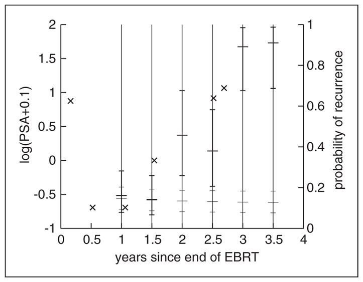
Example of individual predicted probability of clinical recurrence within 3 years updated every 6 months from the 4-class JLCM (bold plain line) and the 1-class JLCM (plain line) for a subject who recurred 3.8 years after the end of EBRT and had T-stage=2 Gleason=7, iPSA=9.7 ng/mL and repeated PSA measurements denoted by ×.

Predictive accuracy can be evaluated on the same dataset as used for estimation using the cross-validated estimate of EPOCE. Graph 3 displays (A) this estimate, the CVPOL_a, computed for a time at prediction from 1 to 6 years after EBRT from the different JLCM and SREM, as well as (B) the differences in CVPOL_a between the 4-class JLCM and, respectively, the best SREM and the 2- and 3-class JLCM with 95% tracking intervals. JLCM with at least three latent classes have a better predictive accuracy than the 1-class prognostic model not accounting for PSA repeated measures. This illustrates the relevance of updating the risk of recurrence using dynamic prognostic tools rather than standard prognostic tools based only on baseline information. Moreover, according to the 95% tracking interval, the 4-class JLCM seems better than the simpler 2-class JLCM at least in the four first years after EBRT where detecting subjects at high risk of recurrence is particularly important. Similarly, the 4-class JLCM also appears better than the SREM (including the PSA current level and slope as covariate) in these four first years after EBRT according to the 95% tracking interval (Figure 3).

Figure 3.

(A) CVPOL_a, cross-validated estimate of EPOCE, computed from the SREM (with current PSA level and current PSA slope included as covariates in the survival model), and from JLCM models with G=1 to G=5 latent classes for times at prediction from 1 to 6 years after EBRT, (B) Differences in EPOCE with 95% tracking interval (TI) on UM dataset (N=459).

In prognostic model development, validation on external data is recommended. We used a second independent dataset (VANC) to compute predictive accuracy measures based on the joint models estimated on UM data. VANC data came from the British Columbia Cancer Agency (Vancouver, Canada).³⁸ Inclusion criteria were the same as in the UM sample. In brief, 719 patients including 126 (17.5%) who had a clinical recurrence were followed-up for a median of 6.48 (IQR=4.28,8.22) years. The mean iPSA on the logarithm scale was 1.97 (SE=0.74), 105 (14.6%) patients had a T-stage of 3 or 4 and, respectively, 145 (20.2%) and 38 (5.3%) patients had a Gleason score of 7 and above 7.

Figure 4 displays the estimate of EPOCE, the MPOL, and its differences, as well as two estimates of the Integrated Brier Score (IBS), computed using the data-based approach defined in equation (12) or the model-based approach defined in equation (13). The two IBS estimates gave roughly the same results, both indicating a reduced error of prediction during the entire follow-up for JLCM with at least three latent classes and the SREM. According to EPOCE, the SREM and the JLCM from two to five latent classes seemed to have relatively close predictive accuracies. But difference in EPOCE between the 4-class JLCM and either the 2-class JLCM or (to a lesser extent) the SREM remained substantial in the first years of prediction according to the 95% tracking intervals of EPOCE differences, since these intervals exclude zero.

Figure 4.

Predictive accuracy measures at times at prediction from 1 to 6 years after EBRT computed on VANC dataset (N=719) from joint models estimated on UM dataset: (A) EPOCE estimate, (B) difference in EPOCE and 95% tracking interval (TI), (C) data-based estimate of Integrated Brier Score (IBS), and (D) model-based estimate of IBS. The censoring distribution for the IBS data-based estimate is modelled in a semi-parametric proportional hazard model with Gleason, T-stage, iPSA as covariates. SREM refers to the SREM with current PSA level and slope included as covariates in the survival model while G=1 to G=5 refer to JLCM with G=1 to G=5 latent classes.

6 Concluding remarks

Joint latent class models have received much less attention than shared-random-effect models in the joint modelling literature. Yet, although they may not be suitable to evaluate specific assumptions regarding the link between a longitudinal marker and the time to an event, as in surrogate marker evaluation for example, they offer a flexible framework to model the joint distribution of the longitudinal marker and the time-to-event. The JLCM summarises their dependency by the assumed categorical structure explaining heterogeneous profiles of the marker and risks of the event, while the SREM summarises their dependency by specific a priori determined functions of the marker trajectory. This characteristic of the JLCM, which may restrict its usefulness to descriptive analyses, can turn out to be a great asset in prediction studies as it approximates any structure, even complex, of the correlated data without a priori assumption. As an example, in the illustration about prostate cancer progression after radiation therapy, the JLCM with four latent classes gave a substantial gain in goodness-of-fit compared to the SREM.

Evaluating predictive accuracy of prognostic tools derived from joint models is not straightforward because of the censoring process and of the dynamic nature of the prognostic tool. We reviewed two types of predictive accuracy measures, quadratic errors of prediction and expected prognostic observed cross-entropy, and showed how to compute them with a JLCM and with a SREM. The quadratic error of prediction (or Brier Score) is reasonably well known in the prediction literature, but its estimates rely on assumptions regarding the censoring distribution and the window of horizons in which predictive accuracy is evaluated. In contrast, the expected prognostic observed cross-entropy does not require any assumption regarding the censoring distribution, makes use of all the available information from the time at prediction, and provides a tracking interval for the difference of predictive accuracy that makes the comparison of models possible.

In this article we illustrated the methods using a dataset that was small relative to the complexity of the JLCM that included a large number of parameters. This was for illustrative purposes only. It emphasised the flexibility of this approach to include covariates in different ways, and model the dependency (stratification of the risks of events over classes for example). However, it produced large credibility bands for the individual predicted probabilities and large tracking intervals for the EPOCE differences. In practice, when developing dynamic predictive tools and applying such joint models, estimation on large datasets (possibly pooled datasets) is recommended to ensure precise estimates of the model parameters and less uncertainty in the individual predictions. Moreover, validation of the dynamic predictive tools on different external datasets (rather than a single one as in this example) with different characteristics would be recommended. Further validation of dynamic predictive tools from a joint model on external data, and comparison with other approaches such as survival models including the previous biomarker measures are described in Proust-Lima and Taylor.²

Finally, we note that all the models fitted in the illustration were estimated using available R packages: lcmm package for JLCM ( Jointlcmm and epoce functions) and JM package for SREM. Other codes for the computation of predictive accuracy measures are available on request from the authors.

References

- 1.Wulfsohn MS, Tsiatis AA. A joint model for survival and longitudinal data measured with error. Biometrics. 1997;53(1):330–339. [PubMed] [Google Scholar]
- 2.Proust-Lima C, Taylor JMG. Development and validation of a dynamic prognostic tool for prostate cancer recurrence using repeated measures of post-treatment PSA: a joint modelling approach. Biostatistics. 2009;10:535–549. doi: 10.1093/biostatistics/kxp009. [DOI] [PMC free article] [PubMed] [Google Scholar]
- 3.Yu M, Taylor JMG, Sandler HM. Individual prediction in prostate cancer studies using a joint longitudinal survival-cure model. J Am Stat Assoc. 2008;103:178–187. [Google Scholar]
- 4.Prentice RL. Covariate measurement errors and parameter estimation in cox’s failure time regression model. Biometrika. 1982;69(2):331–342. [Google Scholar]
- 5.Taylor JMG, Yu M, Sandler HM. Individualized predictions of disease progression following radiation therapy for prostate cancer. J Clin Oncol. 2005;23(4):816–825. doi: 10.1200/JCO.2005.12.156. [DOI] [PubMed] [Google Scholar]
- 6.Henderson R, Diggle P, Dobson A. Joint modelling of longitudinal measurements and event time data. Biostatistics. 2000;1(4):465–480. doi: 10.1093/biostatistics/1.4.465. [DOI] [PubMed] [Google Scholar]
- 7.Rizopoulos D. Dynamic predictions and prospective accuracy in joint models for longitudinal and time-to-event data. Biometrics. 2011;67(3):819–829. doi: 10.1111/j.1541-0420.2010.01546.x. [DOI] [PubMed] [Google Scholar]
- 8.Huang X, Li G, Elashoff RM, Pan J. A general joint model for longitudinal measurements and competing risks survival data with heterogeneous random effects. Lifetime Data Anal. 2011;17(1):80–100. doi: 10.1007/s10985-010-9169-6. [DOI] [PMC free article] [PubMed] [Google Scholar]
- 9.Rizopoulos D, Ghosh P. A bayesian semiparametric multivariate joint model for multiple longitudinal outcomes and a time-to-event. Stat Med. 2011;30(12):1366–1380. doi: 10.1002/sim.4205. [DOI] [PubMed] [Google Scholar]
- 10.Vermunt JK, Magidson J. Latent class models for classification. Comput Stat Data Anal. 2003;41(3–4):531–537. [Google Scholar]
- 11.Lin H, Turnbull BW, McCulloch CE, Slate EH. Latent class models for joint analysis of longitudinal biomarker and event process data: application to longitudinal prostate-specific antigen readings and prostate cancer. J Am Stat Assoc. 2002;97:53–65. [Google Scholar]
- 12.Proust-Lima C, Joly P, Jacqmin-Gadda H. Joint modelling of multivariate longitudinal outcomes and a time-to-event: a nonlinear latent class approach. Comput Stat Data Anal. 2009;53(4):1142–1154. [Google Scholar]
- 13.Garre FG, Zwinderman AH, Geskus RB, Sijpkens YWJ. A joint latent class changepoint model to improve the prediction of time to graft failure. J Roy Stat Soc Ser A. 2008;171(1):299–308. [Google Scholar]
- 14.Beunckens C, Molenberghs G, Verbeke G, Mallinckrodt C. A latent-class mixture model for incomplete longitudinal gaussian data. Biometrics. 2008;64(1):96–105. doi: 10.1111/j.1541-0420.2007.00837.x. [DOI] [PubMed] [Google Scholar]
- 15.Dantan E, Proust-Lima C, Letenneur L, Jacqmin-Gadda H. Pattern mixture models and latent class models for the analysis of multivariate longitudinal data with informative dropouts. Int J Biostat. 2008;4 doi: 10.2202/1557-4679.1088. Article 14. [DOI] [PubMed] [Google Scholar]
- 16.Zhang S, Müller P, Do KA. A Bayesian semiparametric survival model with longitudinal markers. Biometrics. 2010;66(2):435–443. doi: 10.1111/j.1541-0420.2009.01276.x. [DOI] [PMC free article] [PubMed] [Google Scholar]
- 17.Diggle PJ, Sousa I, Chetwynd AG. Joint modelling of repeated measurements and time-to-event outcomes: the fourth Armitage lecture. Stat Med. 2008;27(16):2981–2998. doi: 10.1002/sim.3131. [DOI] [PubMed] [Google Scholar]
- 18.Laird NM, Ware JH. Randomeffects models for longitudinal data. Biometrics. 1982;38:963–974. [PubMed] [Google Scholar]
- 19.Marquardt D. An algorithm for leastsquares estimation of nonlinear parameters. SIAM J Appl Math. 1963;11:431–441. [Google Scholar]
- 20.Stephens M. Dealing with label switching in mixture models. J Roy Stat Soc Ser B. 2000;62(4):795–809. [Google Scholar]
- 21.Redner RA, Walker FH. Mixture densities, maximum likelihood and the EM algorithm. SIAM Rev. 1984;26(2):195–239. [Google Scholar]
- 22.Hipp JR, Bauer DJ. Local solutions in the estimation of growth mixture models. Psychol Meth. 2006;11:36–53. doi: 10.1037/1082-989X.11.1.36. [DOI] [PubMed] [Google Scholar]
- 23.Biernacki C, Celeux G, Govaert G. Choosing starting values for the EM algorithm for getting the highest likelihood in multivariate Gaussian mixture models. Comput Stat Data Anal. 2003;41(3–4):561–575. [Google Scholar]
- 24.Hawkins DS, Allen DM, Stromberg AJ. Determining the number of components in mixtures of linear models. Comput Stat Data Anal. 2001;38(1):15–48. [Google Scholar]
- 25.Han J, Slate EH, Pena EA. Parametric latent class joint model for a longitudinal biomarker and recurrent events. Stat Med. 2007;26(29):5285–5302. doi: 10.1002/sim.2915. [DOI] [PMC free article] [PubMed] [Google Scholar]
- 26.Rizopoulos D. JM: An R package for the joint modelling of longitudinal and time-to-event data. J Stat Softw. 2010;35(9):1–33. [Google Scholar]
- 27.Dobson A, Henderson R. Diagnostics for joint longitudinal and dropout time modeling. Biometrics. 2003;59:741–751. doi: 10.1111/j.0006-341x.2003.00087.x. [DOI] [PubMed] [Google Scholar]
- 28.Lin H, McCulloch CE, Rosenheck RA. Latent pattern mixture models for informative intermittent missing data in longitudinal studies. Biometrics. 2004;60(2):295–305. doi: 10.1111/j.0006-341X.2004.00173.x. [DOI] [PubMed] [Google Scholar]
- 29.Jacqmin-Gadda H, Proust-Lima C, Taylor JMG, Commenges D. Score test for conditional independence between longitudinal outcome and time to event given the classes in the joint latent class model. Biometrics. 2010;66(1):11–19. doi: 10.1111/j.1541-0420.2009.01234.x. [DOI] [PubMed] [Google Scholar]
- 30.Muthén B, Brown CH, Masyn K, et al. General growth mixture modeling for randomized preventive interventions. Biostatistics. 2002;3(4):459–475. doi: 10.1093/biostatistics/3.4.459. [DOI] [PubMed] [Google Scholar]
- 31.Rizopoulos D, Verbeke G, Molenberghs G. Multiple-imputation-based residuals and diagnostic plots for joint models of longitudinal and survival outcomes. Biometrics. 2010;66(1):20–29. doi: 10.1111/j.1541-0420.2009.01273.x. [DOI] [PubMed] [Google Scholar]
- 32.Henderson R, Diggle P, Dobson A. Identification and efficacy of longitudinal markers for survival. Biostatistics. 2002;3(1):33–50. doi: 10.1093/biostatistics/3.1.33. [DOI] [PubMed] [Google Scholar]
- 33.Schoop R, Schumacher M, Graf E. Measures of prediction error for survival data with longitudinal covariates. Biometrical J. 2011;53(2):275–293. doi: 10.1002/bimj.201000145. [DOI] [PubMed] [Google Scholar]
- 34.Commenges D, Liquet B, Proust-Lima C. Choice of prognostic estimators in joint models by estimating differences of expected conditional Kullback-Leibler risks. Biometrics. 2012 doi: 10.1111/j.1541-0420.2012.01753.x. (in press) [DOI] [PubMed] [Google Scholar]
- 35.Gerds TA, Schumacher M. Consistent estimation of the expected brier score in general survival models with right-censored event times. Biometrical J. 2006;48(6):1029–1040. doi: 10.1002/bimj.200610301. [DOI] [PubMed] [Google Scholar]
- 36.Rosthoj S, Keiding N. Explained variation and predictive accuracy in general parametric statistical models: the role of model misspecification. Life-time Data Anal. 2004;10(4):461–472. doi: 10.1007/s10985-004-4778-6. [DOI] [PubMed] [Google Scholar]
- 37.Gerds TA, Schumacher M. Efrontype measures of prediction error for survival analysis. Biometrics. 2007;63(4):1283–1287. doi: 10.1111/j.1541-0420.2007.00832.x. [DOI] [PubMed] [Google Scholar]
- 38.Pickles T, Kim-Sing C, Morris W, et al. Evaluation of the Houston biochemical relapse definition in men treated with prolonged neoadjuvant and adjuvant androgen ablation and assessment of followup lead-time bias. Int J Radiat Oncol Biol Phys. 2003;57:1118. doi: 10.1016/s0360-3016(03)00439-5. [DOI] [PubMed] [Google Scholar]