Quality control, imputation and analysis of genome-wide genotyping data from the Illumina HumanCoreExome microarray

Abstract

The decreasing cost of performing genome-wide association studies has made genomics widely accessible. However, there is a paucity of guidance for best practice in conducting such analyses. For the results of a study to be valid and replicable, multiple biases must be addressed in the course of data preparation and analysis. In addition, standardizing methods across small, independent studies would increase comparability and the potential for effective meta-analysis. This article provides a discussion of important aspects of quality control, imputation and analysis of genome-wide data from a low-coverage microarray, as well as a straight-forward guide to performing a genome-wide association study. A detailed protocol is provided online, with example scripts available at https://github.com/JoniColeman/gwas_scripts .

Introduction

Genome-wide association studies (GWAS) are widely used to assess the impact of common genetic variation on a variety of phenotypes [ 1 , 2 ]. Low-cost microarrays designed to assay thousands of variants and to be imputable to millions, such as the Illumina HumanCoreExome microarray (Illumina, San Diego, CA, USA), have increased the accessibility of this technology. Although the rapid development and falling cost of whole-genome sequencing is likely to reduce the use of GWAS in the long term, the costs of running a GWAS are currently an order of magnitude smaller than those for sequencing, suggesting GWAS will remain an important technique into the near future [ 3 ].

However, there is a paucity of information on best practice for using the data resulting from microarray-based genotyping. Excellent theoretical and practical protocols for the quality control of genome-wide genotype data exist [ 4 , 5 ], and most commonly used software have well-constructed user manuals, but structured advice to guide analysis is missing from the literature. To date, a considerable proportion of the analysis of such data has been concentrated within large consortia (such as the Psychiatric Genomics Consortium), with experienced analysts and in-house protocols [ 6 , 7 ]. However, such guidance is not easily available to groups outside these consortia. As the accessibility of genome-wide data increases, so must the accessibility of advice on its analysis. Furthermore, a standardized approach would increase comparability between studies, facilitating further investigations such as meta-analysis and augmenting the value of each individual study [ 8 ].

The choices made in conducting the analysis of genotype data affect the final result. At worst, poor quality control can lead to systematic biases in outcome and increased false-positive (and false-negative) associations [ 4 ]. However, the effects can be more nuanced; for example, association testing using a mixed linear model may use a genetic relatedness matrix (GRM) to control for gross genetic similarity between individuals [ 9 , 10 ]. The precise pairwise relationships will differ subtly depending on whether the GRM is made using the genotype data before or after imputation (as well as on the programme used), and so the results of the association study will also differ slightly. Neither choice in this context is wrong, but the choice made has consequences, and as such needs to be considered and reported [ 11 ].

Recently, we performed the first genome-wide association study of response to cognitive behavioural therapy, using the HumanCoreExome microarray (Coleman et al, Under Review). In this protocol, we have used that experience to provide suggestions for the quality control, imputation and analysis of data from this microarray, assuming careful recalling of the raw intensity data has been performed. The steps are likely to be applicable to data from other arrays, with the caveat that differences in array content may require alteration of the various thresholds discussed. The analysis of genome-wide data remains a data-driven activity, and, where appropriate, we have provided advice on making informed choices from the data. Furthermore, we recommend consulting graphical representations of the data when defining thresholds.

Pre-analytical procedures: genotyping, calling and recalling

This protocol describes the basic analytical steps required to conduct a genome-wide association study; it is expected that DNA genotyping and genotype recalling have already been performed. In this context, genotyping refers to the hybridization of genomic DNA to oligonucleotide probes targeted at a polymorphic region, and the extension of these probes to encompass this region. This extension uses chemically labelled nucleotides that are specific to the different alleles of the polymorphism and that bind either red or green fluorescent agents, which can be read using a fluorescence-sensitive scanner. The end product of genotyping is the raw intensity data of these fluorescent agents at each polymorphic site [ 12 ]. To determine the identity of the alleles at these sites, the raw intensity data must be called—clusters of samples with similar intensities are identified, and the clusters are labelled according to the design of the microarray. This initial calling is performed by automated software—however, the algorithms to perform this calling sometimes fail to identify valid clusters, especially when patterns of clustering are unusual. As such, some clusters must be identified by manual recalling by a bioinformatician. Recalling is an extremely important step—badly called genotypes create biases that severely impair the quality control and analysis of data. The complexities of genotyping and recalling are beyond the scope of this protocol, but guidance is available from array manufacturers and as referenced in the Supplementary Data [ 13 ].

Considerations in conducting a study

The value of any finding in molecular genetics is reliant on the ability to replicate it in an independent cohort, and the first step to successful replication is to minimize the likelihood that reported findings are false positives. Given that thousands of variants are assessed in a GWAS, and the potential for random error in genotyping and recalling (as discussed above), it is necessary to impose stringent thresholds on the quality of data to be taken forward to analysis [ 4 ]. Pre-analytical steps partly inform these thresholds. When a more variable method of collection has been used, it is advisable to consider more stringent quality control parameters; for example, collection using buccal swabs produces poorer quality DNA than extractions from whole blood or saliva [ 14 ].

Quality control: selecting variants by allele frequency

Following genotyping and the recalling of genotypes, most GWAS studies begin by filtering the variants by the frequency of the less-common allele (minor allele frequency or MAF). Variant MAF has many effects on later analysis, as allele frequency is associated with time since mutation, the structure of local linkage disequilibrium (LD) and the relative size of the association statistic [ 15 , 16 ]. The chances of an error in genotype calling increase with decreasing MAF, as the certainty of manual and automatic clustering falls with fewer variants in each cluster [ 17 ]. At the most extreme level, if all but one variant cluster together, it is difficult to assess whether the lone variant is truly a different genotype, or whether it is a missed call. For this reason, the rarest variants should be discarded from the analysis. What constitutes ‘rare' depends on the size of the studied cohort—assuming perfect Hardy–Weinberg equilibrium, the minor allele of a variant with MAF = 0.1% would be expected to be present in 19 heterozygotes and 1 homozygote in a cohort of 10 000 individuals, but only one or two heterozygotes would be expected in a cohort of 1000 individuals. In smaller cohorts, a more stringent MAF cut-off is recommended, as the minor allele count will be lower, which limits the value of conclusions from the analysis of these variants. For the smallest studies, where fewer than 1000 individuals are investigated, a cut-off of 5% should be considered—this is in line with the analysis program GenAbel, for example, which uses a minor allele count of 5 as its cut-off [ 18 ]. Typically, many studies define rare single nucleotide polymorphisms (SNPs) as having a MAF <1%, which has historical roots in the HapMap project [ 19 ]. It is worth noting that the exonic content of the HumanCoreExome chip was specifically designed to target coding variants, with much of this content having a population MAF <1% [ 17 ]. Therefore, using this microarray in smaller cohorts and imposing a MAF cut-off of 1% or higher will result in discarding most of the exonic content.

Quality control: removing variants and samples with missing data

It is necessary to remove rare variants from GWAS because the certainty of the genotype call is reduced by their low minor allele count. Even in common variants, however, genotyping and genotype recalling are subject to technical error, with the result that a proportion of variants and samples are of low quality, and should be removed from the analysis. Removal of such missing variants and samples is best conducted in an iterative manner, removing variants genotyped in <90% of the samples, then samples with <90% of variants and continuing with increasing stringency to a user-defined final threshold (typically in the range of 95–99% completeness, depending on the required stringency of quality control). This has benefits over removing all variants and samples beneath the final threshold, as fewer samples are lost using the iterative procedure (at the expense of a slight increase in variant exclusions).

Quality control: assessing deviation from Hardy-Weinberg equilibrium

Thresholds that identify missing variants do not necessarily exclude miscalled variants. For example, clustering algorithms can incorrectly define a group of samples as heterozygous. One method to detect this is to evaluate the deviation from Hardy–Weinberg equilibrium at each variant. Although such deviations can be caused by processes that may be of interest within the study, such as selection pressure, the expected size of such deviations is small. Setting the threshold for the P -value of the Hardy–Weinberg test to be low ( P  < 1 × 10 ⁻⁵ ) decreases the probability of excluding deviations that result from processes of interest. In case-control studies, it is recommended to remove SNPs deviant in controls only (this is the default behaviour in PLINK2). Deviations from Hardy–Weinberg equilibrium as a result of genotyping artefacts are not expected to differ between cases and controls, but biologically relevant deviations are more likely to occur in cases [ 5 ]. The threshold for the P -value cut-off can be determined empirically, by examining the spread of P -values from the Hardy–Weinberg test in the data, and selecting a threshold under which there are a greater number of variants than expected by chance (in our experience, with small data sets, this is typically around P  = 1 × 10 ⁻⁵ ).

Quality control: pruning for LD and removing related samples

The initial quality control steps described above correct for the random errors introduced by genotyping and recalling. Further steps are required to address cryptic structure, the presence of similarities between individuals independent of the phenotype under study, which present a source of potential bias in the outcome of association tests. Such structure is commonly envisaged as two interconnected concepts, high relatedness between individuals (determined by the proportion of their genomes identical-by-descent—IBD) and population stratification. The presence of structure is inferred from examining genome-wide genotype data. However, the phenomenon of LD can exaggerate or obscure similarities, as a shared region of high LD results in more shared variants than one of low LD, even if the two regions are the same size. Accordingly, it is necessary to prune the data for LD before assessing IBD and population stratification. This can be achieved using a pairwise comparison method, comparing each possible pair of variants in a given window of variants and removing one of the pair if the LD between them is above a given cut-off. This protocol uses a window of 1500 variants, shifted by 10% for each new round of comparisons, and a threshold of R ² > 0.2. The window size of 1500 variants corresponds to the large, high LD chromosome 8 inversion, while the shift of 10% represents a trade-off between efficiency and thoroughness [ 5 ].

Once an LD-pruned data set is obtained, individuals can be compared pairwise to establish the proportion of variants they share identical-by-state (IBS). Closely related individuals share more of their genome than a randomly chosen pair of individuals from the population, and are likely to be more phenotypically similar. As a result, including closely related individuals can skew analysis; genetic variants shared because of close relatedness can become falsely associated with phenotypic similarity that also results from close relatedness.

With a sufficiently homogeneous cohort assayed at thousands of variants, IBS information can be used to infer variants that are shared identical-by-descent (IBD) [ 20 ]. Individuals with an IBD metric (pi-hat) > 0.1875 (halfway between a second and third degree relative [ 4 ]) should be removed, as well as individuals with unusually high average IBD with all other individuals, which may indicate sample contamination or genotype recalling error leading to too many heterozygote calls [ 20 ]. The IBD threshold suggested here is designed to remove the most closely related individuals, while avoiding removing large numbers of samples through being overly stringent. It is worth noting that some downstream analysis programs impose much more severe IBD cut-offs (GREML estimation in GCTA, which produces an estimate of heritability from all assayed variants, uses 0.025), while other analyses account for between-sample relatedness as part of the analysis [ 9 , 21 ]. What quality control is appropriate depends on the nature of the cohort, the question being asked and the analysis methods intended to be used.

Quality control: confirming sample gender and assessing the inbreeding coefficient

Samples whose reported gender differs from that suggested by their genes are likely to have been assigned the wrong identity. This leads to reduced power, as the sample's genotype becomes effectively randomized in respect to the phenotype. The average homozygosity of variants on the X chromosome (the X-chromosome F statistic) can be used to indicate sample gender. Much as it confounds estimates of IBD, patterns of LD will also impair chromosome-specific (and genome-wide) tests of homozygosity, and so it is necessary to perform this test following pruning for LD. The F statistic is a function of the deviation of the observed number of heterozygote variants from that expected under Hardy–Weinberg equilibrium. In males, F  ≈ 1, because all X chromosome variants are hemizygous, and so no heterozygotes are observed. Females are expected to have lower values of F , distributed normally around 0 [ 22 ]. However, this is an imprecise measure—female subjects with high F have been reported in the 1000 Genomes reference population ( https://www.cog-genomics.org/plink2/basic_stats ). As such, it is recommended that the <0.2  F threshold for females (as used by PLINK) is treated as guidance, and that further checks (such as counting the number of Y chromosome SNPs with data) are made, and that the phenotypic gender of discordant samples is confirmed with the collecting site where possible [ 20 , 23 ].

In addition to using a chromosome-specific homozygosity check to confirm gender, a whole-genome F should also be calculated. This statistic is also referred to as an ‘inbreeding coefficient', as inbreeding results in reduced numbers of heterozygotes. Individuals with particularly high or low inbreeding coefficients should be removed from analyses, as this is likely to be an artefact caused by genotyping error. However, caution is advised when studying cohorts in which consanguineous relationships are common, as high inbreeding coefficients are expected in these samples.

Quality control: controlling for population stratification

Similarities exist between the false genotype–phenotype correlations created by close between-sample relatedness and those created by population stratification, where phenotypic and genotypic similarity are correlated because of geographical location, rather than a true association. A variety of methods exist to control for population stratification, of which the most common is to perform principal component analysis on the genome-wide data, and then use the resulting components as covariates in association analysis. However, there is little guidance as to which components to choose, and this is often determined empirically in individual studies through piecemeal inclusion of principal components into the analysis until measures of genomic inflation fall below a chosen threshold (usually until the genomic inflation statistic lambda ≈ 1 [ 24 ]). We suggest an alternative, regressing principal components on outcome directly, and keeping only those that explain variance in the outcome at a rate above chance for use as covariates in the GWAS. This then leaves the question of what should be done if no component is associated with outcome. Recent computational developments have enabled an alternative means of control through the construction of genomic relatedness matrices [ 11 ]. This method compares the deviation of each individual from the population mean at each variant in the data set, and then compares individuals pairwise to establish a value for overall genetic similarity. This can then be entered into the analysis as a random variable in a mixed linear regression, and has the benefit of capturing population variance at a finer-scale level than principal component analysis [ 11 ] (for an in-depth discussion of the comparison between principal component analysis and genetic relatedness matrices, see [ 25 ]).

Imputation to the 1000 Genomes reference population

The main benefits of the HumanCoreExome as a low-cost microarray are twofold. First, the exonic content allows rare coding variation to be assayed in large numbers of samples without the high costs of sequencing these variants [ 26 ]. However, this relies on large sample sizes to allow for reliable calling of the genotypes. The value of the array in smaller cohorts is in providing an inexpensive means to assay thousands of variants that are in high LD with a considerably greater number. To make effective use of the array in this manner requires imputation of the data to a reference population, most commonly the 1000 Genomes Reference [ 27 ]. However, the advent of large-scale sequencing studies such as UK10K ( http://www.uk10k.org/ ) and Genomics England ( http://www.genomicsengland.co.uk/ ), and the increasing availability of sequence data on specific populations, is likely to result in alterations to imputation practice in the near future.

The Supplementary Data uses IMPUTE2 [ 28 , 29 ] to impute to the full 1000 Genomes Reference population. This is performed without pre-phasing, as there is evidence that this is the most accurate method (albeit somewhat slower than pre-phasing; http://blog.goldenhelix.com/?p=1911 ). It also assumes access to a multi-node computing cluster, although jobs could be run sequentially (with considerable increases in computational time). The imputed data that result from these methods are provided in a probabilistic ‘dosage' format, which is an attractive format from a statistical perspective, as it allows for the variable certainty of each imputed call to be considered within the association model. Programs exist that allow for the direct use of dosage data in association analyses, such as SNPTEST and ProbABEL ( https://mathgen.stats.ox.ac.uk/genetics_software/snptest/old/snptest.html ; [ 30 ]). However, this format remains computationally burdensome at present—for example, it is not yet possible to store dosage data as a file input type in PLINK, akin to the PLINK binary format. As such, the protocol converts these probabilistic calls to binary ‘hard' calls, marking less-certain calls as missing. This increases downstream flexibility at the expense of losing the more informative probabilistic calls. With increasing computational sophistication, it is likely that the use of dosage data as an input file type will become possible and commonplace; to this end, readers are advised to consult the PLINK2 website ( https://www.cog-genomics.org/plink2/ ).

Post-imputation quality control: monomorphic, rare and missing variants

Following imputation, data are provided for a large number of variants (83 million in the latest release of the 1000 Genomes Project). As such, there is a necessity to perform post-imputation quality control. Monomorphic variants should be removed (MAF = 0), as well as variants that are extremely rare in the cohort (see the earlier discussion of MAF removals). IMPUTE2 provides an ‘info' score related to the quality of the imputation for each variant. Different sources recommend different thresholds to exclude poorly imputed data. The selection of this threshold should be made taking into account the overall quality of the data (poor-quality data require greater quality control, and so a higher info threshold should be used). The best method is to plot a frequency curve ( Figure 1 ) or cumulative distribution ( Figure 2 ) of the info score and assign the threshold at the inflexion point. For example, the graphs below show most of the worst-performing variants have info <0.15, and there is an enrichment of high-quality variants with info >0.85. The threshold chosen should fall between these two. There is a relationship between MAF and info, and it is valuable to examine these metrics together—rarer variants usually show lower info scores, and often the appropriate cut-off is obvious from plotting info in MAF bins ( Figure 3 ). In this example, a MAF cut-off of 0.01 appears to remove most of the SNPs with low info scores. Finally, it is necessary to exclude variants missing in multiple samples when using hard-called data, as variants imputed with a certainty below threshold are marked as missing rather than being excluded. Defining the threshold for completeness again benefits from plotting the data: in the example shown in Figure 4 , a cut-off of 98% completeness appears to be an acceptable trade-off between retaining variants in the analysis and reducing the variation in sample size between analyses of each variant. Again, the threshold chosen should be informed by the necessary stringency of the quality control and the proposed downstream analysis.

Figure 1.

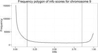
Frequency polygon showing the number of variants at each info value post-imputation, including poor-quality variants to be excluded (info <0.15) and higher-quality variants that should be kept (info >0.85).

Figure 2.

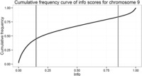
Cumulative frequency curve showing the same data as Figure 1 .

Figure 3.

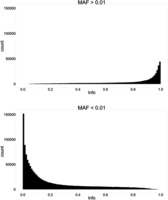
Histograms of the info metric of imputed variants on chromosome 9, split by MAF at 0.01.

Figure 4.

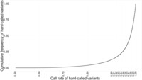
Cumulative frequency plot of call rate of hard-called imputed SNPs (genome wide).

Association analyses

The final step presented in this protocol is to perform the association analysis itself. The exact analysis performed depends on the research question being investigated and the covariates included. The flexibility of PLINK2 for running multiple statistical models and including covariates in a variety of different ways, coupled with a user-friendly implementation, arguably means it remains the first choice for performing analyses. However, many other programs exist, and it is worthwhile investigating whether a piece of software particularly suited to the planned analysis is available. The introduction of mixed linear model association analysis is an example of this, allowing for an approach to control for population structure that is as yet not available in PLINK2, although the implementation of GCTA code into PLINK2 is expected in the near future [ 9 , 11 , 23 ]. The development of association analysis software is an active area of research, with programs such as FasT-LMM and BOLT-LMM providing alternative implementations to GCTA [ 31 , 32 ].

Conclusion

GWAS remains a valuable technique for understanding the role of genetic variants in explaining phenotypic variation, and is likely to persist as an affordable alternative as the field moves into the sequencing era. The analysis of thousands of variants allows novel findings to be made, and targets for replication to be established. Minimizing false-positive findings from GWAS will allow for more efficient use of research effort through reducing the likelihood of failed replication.

This protocol is intended as an introduction to the concepts and processes of analysing novel data from microarrays—quality control, imputation and analysis are areas of constant statistical and computational innovation, and advanced techniques that may be more appropriate for a given data set are regularly posited in the literature. We hope that the provision of this simple protocol will ensure the general standard of GWAS remains high, and will simplify the combination of independent studies into the collaborative meta-analyses that have become a hallmark of success in genomics.

Key Points

• Replication, including combining individual studies in meta-analyses is central to genomics.

• Well-executed recalling and quality control of genotype data reduces biases within GWAS studies and increases the probability of successful replication.

• Quality control, imputation and analysis of genotype data are data-driven activities.

• The protocol provided with this article provides a straightforward introduction to the basics of GWAS that will increase standardization of GWAS studies between different groups.

• Example scripts are provided at https://github.com/JoniColeman/gwas_scripts .

Funding

This study presents independent research part-funded by the National Institute for Health Research Biomedical Research Centre at South London and Maudsley NHS Foundation Trust and King’s College London. The views expressed are those of the authors and not necessarily those of the NHS, the NIHR or the Department of Health. JRIC's PhD is partly funded by the Institute of Psychiatry, Psychology and Neuroscience, and partly by the Alexander von Humboldt Foundation.

References

- 1. Hofker MH, Fu J, Wijmenga C . The genome revolution and its role in understanding complex diseases . Biochim Biophys Acta 2014. ; 1842 : 1889 – 95 . [DOI] [PubMed] [Google Scholar]
- 2. Visscher Peter M, Brown Matthew A, McCarthy Mark I, et al. . Five years of GWAS discovery . Am J Hum Genet 2012. ; 90 : 7 – 24 . [DOI] [PMC free article] [PubMed] [Google Scholar]
- 3. Katsanis SH, Katsanis N . Molecular genetic testing and the future of clinical genomics . Nat Rev Genet 2013. ; 14 : 415 – 26 . [DOI] [PMC free article] [PubMed] [Google Scholar]
- 4. Anderson CA, Pettersson FH, Clarke GM, et al. . Data quality control in genetic case-control association studies . Nat Protoc 2010. ; 5 : 1564 – 73 . [DOI] [PMC free article] [PubMed] [Google Scholar]
- 5. Weale ME . Quality control for genome-wide association studies . Methods Mol Biol 2010. ; 628 : 341 – 72 . [DOI] [PubMed] [Google Scholar]
- 6. Corvin A, Craddock N, Sullivan PF . Genome-wide association studies: a primer . Psychol Med 2010. ; 40 : 1063 – 77 . [DOI] [PMC free article] [PubMed] [Google Scholar]
- 7. Sullivan PF . The psychiatric GWAS consortium: big science comes to psychiatry . Neuron 2010. ; 68 : 182 – 6 . [DOI] [PMC free article] [PubMed] [Google Scholar]
- 8. de Bakker PIW, Ferreira MAR, Jia X, et al. . Practical aspects of imputation-driven meta-analysis of genome-wide association studies . Hum Mol Genet 2008. ; 17 : R122 – 8 . [DOI] [PMC free article] [PubMed] [Google Scholar]
- 9. Yang J, Lee SH, Goddard ME, et al. . GCTA: a tool for genome-wide complex trait analysis . Am J Hum Genet 2011. ; 88 : 76 – 82 . [DOI] [PMC free article] [PubMed] [Google Scholar]
- 10. Kang HM, Sul JH, Service SK, et al. . Variance component model to account for sample structure in genome-wide association studies . Nat Genet 2010. ; 42 : 348 – 54 . [DOI] [PMC free article] [PubMed] [Google Scholar]
- 11. Yang J, Zaitlen NA, Goddard ME, et al. . Advantages and pitfalls in the application of mixed-model association methods . Nat Genet 2014. ; 46 : 100 – 6 . [DOI] [PMC free article] [PubMed] [Google Scholar]
- 12. Steemers FJ, Chang W, Lee G, et al. . Whole-genome genotyping with the single-base extension assay . Nat Methods 2006. ; 3 : 31 – 3 . [DOI] [PubMed] [Google Scholar]
- 13. Gunderson KL, Steemers FJ, Ren H, et al. . Whole-genome genotyping . In: Kimmel A, Oliver B. (eds). Methods in Enzymology . San Diego, CA: : Academic Press; , 2006. , 359 – 76 . [DOI] [PubMed] [Google Scholar]
- 14. Hansen TvO, Simonsen MK, Nielsen FC, et al. . Collection of blood, saliva, and buccal cell samples in a pilot study on the danish nurse cohort: comparison of the response rate and quality of genomic DNA . Cancer Epidemiol Biomarkers Prev 2007. ; 16 : 2072 – 6 . [DOI] [PubMed] [Google Scholar]
- 15. Kruglyak L . Prospects for whole-genome linkage disequilibrium mapping of common disease genes . Nat Genet 1999. ; 22 : 139 – 44 . [DOI] [PubMed] [Google Scholar]
- 16. Reich DE, Goldstein DB . Detecting association in a case-control study while correcting for population stratification . Genet Epidemiol 2001. ; 20 : 4 – 16 . [DOI] [PubMed] [Google Scholar]
- 17. Goldstein JI, Crenshaw A, Carey J, et al. . zCall: a rare variant caller for array-based genotyping: genetics and population analysis ., Bioinformatics 2012. ; 28 : 2543 – 5 . [DOI] [PMC free article] [PubMed] [Google Scholar]
- 18. Aulchenko YS, Ripke S, Isaacs A, et al. . GenABEL: an R library for genome-wide association analysis . Bioinformatics 2007. ; 23 : 1294 – 6 . [DOI] [PubMed] [Google Scholar]
- 19. The International HapMap C . A haplotype map of the human genome . Nature 2005. ; 437 : 1299 – 320 . [DOI] [PMC free article] [PubMed] [Google Scholar]
- 20. Purcell S, Neale B, Todd-Brown K, et al. . PLINK: a tool set for whole-genome association and population-based linkage analyses . Am J Hum Genet 2007. ; 81 : 559 – 75 . [DOI] [PMC free article] [PubMed] [Google Scholar]
- 21. Visscher PM, Andrew T, Nyholt DR . Genome-wide association studies of quantitative traits with related individuals: little (power) lost but much to be gained . Eur J Hum Genet 2008. ; 16 : 387 – 90 . [DOI] [PubMed] [Google Scholar]
- 22. Hartl D, Clark HG. Principles of population genetics . Sunderland, MA: : Sinauer Associates; , 2006. . [Google Scholar]
- 23. Chang C, Chow C, Tellier L, et al. . Second-generation PLINK: rising to the challenge of larger and richer datasets . GigaScience 2015. ; 4 : 7 . [DOI] [PMC free article] [PubMed] [Google Scholar]
- 24. Dadd T, Weale ME, Lewis CM . A critical evaluation of genomic control methods for genetic association studies . Genet Epidemiol 2009. ; 33 : 290 – 8 . [DOI] [PubMed] [Google Scholar]
- 25. Zhang Y, Pan W . Principal component regression and linear mixed model in association analysis of structured samples: competitors or complements? Genet Epidemiol 2014. ; 39 : 149 – 55 . [DOI] [PMC free article] [PubMed] [Google Scholar]
- 26. Wagner MJ . Rare-variant genome-wide association studies: a new frontier in genetic analysis of complex traits . Pharmacogenomics 2013. ; 14 : 413 – 24 . [DOI] [PubMed] [Google Scholar]
- 27. 1000 Genomes Consortium . An integrated map of genetic variation from 1,092 human genomes . Nature 2012. ; 491 : 56 – 65 . [DOI] [PMC free article] [PubMed] [Google Scholar]
- 28. Howie B, Fuchsberger C, Stephens M, et al. . Fast and accurate genotype imputation in genome-wide association studies through pre-phasing . Nat Genet 2012. ; 44 : 955 – 9 . [DOI] [PMC free article] [PubMed] [Google Scholar]
- 29. Howie BN, Donnelly P, Marchini J . A flexible and accurate genotype imputation method for the next generation of genome-wide association studies . PLoS Genet 2009. ; 5 : e1000529 . [DOI] [PMC free article] [PubMed] [Google Scholar]
- 30. Aulchenko Y, Struchalin M, van Duijn C . ProbABEL package for genome-wide association analysis of imputed data . BMC Bioinformatics 2010. ; 11 : 134 . [DOI] [PMC free article] [PubMed] [Google Scholar]
- 31. Loh PR, Tucker G, Bulik-Sullivan BK, et al. . Efficient Bayesian mixed-model analysis increases association power in large cohorts . Nat Genet 2015. ; 47 : 484 – 90 . [DOI] [PMC free article] [PubMed] [Google Scholar]
- 32. Lippert C, Listgarten J, Liu Y, et al. . FaST linear mixed models for genome-wide association studies . Nat Methods 2011. ; 8 : 833 – 5 . [DOI] [PubMed] [Google Scholar]
Associated Data
This section collects any data citations, data availability statements, or supplementary materials included in this article.