Direct AUC optimization of regulatory motifs

Abstract

Motivation

The discovery of transcription factor binding site (TFBS) motifs is essential for untangling the complex mechanism of genetic variation under different developmental and environmental conditions. Among the huge amount of computational approaches for de novo identification of TFBS motifs, discriminative motif learning (DML) methods have been proven to be promising for harnessing the discovery power of accumulated huge amount of high-throughput binding data. However, they have to sacrifice accuracy for speed and could fail to fully utilize the information of the input sequences.

Results

We propose a novel algorithm called CDAUC for optimizing DML-learned motifs based on the area under the receiver-operating characteristic curve (AUC) criterion, which has been widely used in the literature to evaluate the significance of extracted motifs. We show that when the considered AUC loss function is optimized in a coordinate-wise manner, the cost function of each resultant sub-problem is a piece-wise constant function, whose optimal value can be found exactly and efficiently. Further, a key step of each iteration of CDAUC can be efficiently solved as a computational geometry problem. Experimental results on real world high-throughput datasets illustrate that CDAUC outperforms competing methods for refining DML motifs, while being one order of magnitude faster. Meanwhile, preliminary results also show that CDAUC may also be useful for improving the interpretability of convolutional kernels generated by the emerging deep learning approaches for predicting TF sequences specificities.

Availability and Implementation

CDAUC is available at: https://drive.google.com/drive/folders/0BxOW5MtIZbJjNFpCeHlBVWJHeW8.

Supplementary information

Supplementary data are available at Bioinformatics online.

1 Introduction

By binding to their genomic target sequences and regulating the expression patterns of genes, transcription factors (TFs) play essential roles in transcriptional regulatory networks which control various cellular and developmental processes. Generally speaking, a TF prefers to bind to similar short sequences (known as TF binding sites, TFBSs) across the genome. In order to untangle the complex mechanism of genetic variation under different developmental and environmental conditions, it is an important first step to discover the underlining overrepresented sequence patterns of TFBSs, which are referred to as TFBS motifs.

In the past decade, due to the rapid development of high-throughput sequencing technology, a variety of experimental methods have been developed to extract TF-DNA binding regions. In particular, ChIP-seq, which combines chromatin immunoprecipitation with high-throughput sequencing, greatly improves the amount and spatial resolution of generated data, both of which are beneficial for the studies of TF binding in vivo. However, ChIP-seq also brings two challenges for motif discovery methods: (i) The enormous amount of potential TF binding regions yielded from a single experiment requires highly scalable motif discovery tools; (ii) Computationally, motif learning methods rank candidate motifs by either implicitly or explicitly contrasting them with a ‘background’ model which describes how the foreground sequences should look like if no motif instance in present there (Valen et al., 2009). Common choices for the background include multinomial or Markov models (Kilpatrick et al., 2014). However, such generic models may fail to capture important properties of real genomic sequences. In addition, a TF could bind alone to some sequences, and yet cooperate with other TFs and bind to other sequences, leading to multiple motifs that each explains only a subset of the foreground set (Mason et al., 2010; Setty and Leslie, 2015). Such subtle signals may not be significantly enriched against a ‘universal’ background, and are thus hard to detect (Bailey and Machanick, 2012; Lesluyes et al., 2014).

Currently, many motif algorithms tailored for high-throughput datasets have been proposed. Among existing approaches, the discriminative motif learning (DML) methods are promising for simultaneously addressing the aforementioned two challenges (Agostini et al., 2014; Bailey, 2011; Mason et al., 2010; Valen et al., 2009; Yao et al., 2013). In contrast to traditional motif learners, DMLs carefully collect a number of real DNA sequences as background, which can better represent the complex and heterogeneous nature of genome sequences and help discern the motif signals of interest, then search for sequence motifs that can discriminate between the positive and negative sets. In addition, by designing the negative dataset in a problem specific manner, DMLs can be also useful for studying context-dependent regulatory activities (Mason et al., 2010).

Computationally, the cost functions DMLs are generally nonconvex, non-differentiable, and even discontinuous, and are thus difficult to optimize. To circumvent such difficulties and improve scalability, current DML methods typically do not search for motif directly over the complete parameter space, but instead adopt approximate schemes that could sacrifice both accuracy and expressive power. For example, the motifs learned by DREME (Bailey, 2011) and MotifRG (Yao et al., 2013) are limited to the discrete IUPAC space, while HOMER (Heinz et al., 2010) chooses to refine motifs by only tuning external parameters. Therefore, although DML algorithms could rapidly identify binding motifs, they may fail to fully utilize the information of the input sequence (Patel and Stormo, 2014).

From a computational point of view, the learning objective of DML methods is essentially the inference of a predictor (represented as a motif) that can discriminate between two input sets (Maaskola and Rajewsky, 2014), which is similar in spirit to several machine learning tasks, especially binary classification and bipartite ranking. For such tasks, the area under the receiver-operating characteristic curve (AUC) figures prominently as the evaluation tool (Gao et al., 2016). Meanwhile, AUC has also been widely used in the literature to measure the significance of extracted motifs (McLeay and Bailey, 2010; Orenstein and Shamir, 2014; Weirauch et al., 2013; Yao et al., 2013).

Given the importance of the AUC metric, several previous studies attempted to investigate whether it may also serve as an alternative criterion for improving the quality of discriminative motif elicitation. Li et al. (2007) proposed GAPWM to utilize AUC for improving the quality of a poorly estimated motif. However, GAPWM is based on genetic algorithm and could be too slow for high-throughput datasets. Instead, Patel et al. (Patel and Stormo, 2014) developed discriminative motif optimizer (DiMO) which can more efficiently refine the quality of raw motifs found by fast DMLs. Experimental evaluations show that it can improve AUC for 90% of the tested TFs, and the magnitude of improvement could be up to 39%. Despite the good performance of DIMO, it achieves efficiency by simply using a fixed heuristic formula to update current motif solutions, whose relationship with the desired AUC objective is hard to characterize. In summary, existing approaches that use AUC as objective for learning motifs either has to rely on heuristic updating rules or is computationally impractical for high-throughput datasets, which indicates a gap in current state of knowledge.

In this paper, we aim at closing this gap by developing a novel algorithm called Coordinate Descent based AUC optimization (CDAUC) for direct maximization of the AUC score of input motifs. The contributions of this paper can be summarized as follows:

1. We show that when the AUC loss function is optimized in a coordinate-wise manner, the cost function of each resultant sub-problem is a piece-wise constant (PCF) function, whose optimal value can be found exactly.

2. To further improve the tractability of CDAUC, we show that the parameter learning of the above mentioned PCF can be cast as computational geometry problem, which is then solved using a specialized data structure called range tree with fractional cascading (De Berg et al., 2000).

3. An efficient parameter setting approach is proposed, which ensures that each sub-problem of the coordinate descent process can be solved in a global-optimal manner.

The remainder of the paper is organized as follows. In Section 2, we formally define the motif optimization problem. As convolutional neural networks (CNNs) are becoming the state-of-the-art approaches for sequence-based prediction of TF binding, we also discuss the differences in terms of problem formulations between DMLs and CNNs, and how CDAUC may also be useful for improving the PWMs learned using CNNs. In Section 3, we present the CDAUC method and discuss its implementation. Experimental configurations and results are given in Section 4.

2 Background

2.1 Problem formulation

As in the general problem setting of discriminative motif learning, we have a set of DNA sequences $\mathcal{T}$ as input, each $S\in \mathcal{T}$ is a string of length $\left|S\right|$ defined over the DNA alphabet. $\mathcal{T}$ is further divided into a positive set $\mathcal{P}$ and a negative set $\mathcal{N}$, and we would like to find the motif that is most significantly enriched in $\mathcal{P}$ relative to $\mathcal{N}$.

As one of the most widely used motif representation, position weight matrices (PWMs) model the motif as $W\in {ℝ}^{|\Sigma |\times l}$, where the entries of each column represent the binding preference for four elements of the DNA alphabet $\Sigma =\{\mathrm{A},\mathrm{C},\mathrm{G},\mathrm{T}\}$ in the corresponding position of the motif. The matching score between any sequence of l letters $s=s_{[1:l]}$ and W is given by (Alipanahi et al., 2015; Patel and Stormo, 2014):

$$f\left(s;W\right)=\sum _{i=1}^l\left(\begin{array}{c}\mathbb{I}\left(s_{\left[i\right]}=\mathrm{A}\right)W_{\left[1,i\right]}+\mathbb{I}\left(s_{\left[i\right]}=\mathrm{C}\right)W_{\left[2,i\right]}+\cdots \\ \cdots \mathbb{I}\left(s_{\left[i\right]}=\mathrm{G}\right)W_{\left[3,i\right]}+\mathbb{I}\left(s_{\left[i\right]}=\mathrm{T}\right)W_{\left[4,i\right]}\end{array}\right),$$ (1)

where $\mathbb{I}(\cdot )$ is the indicator function. For a sequence S that is longer than l, its matching score $f(S;W)$ is the maximal matching score between W and the complete set of l-long subsequences of S, such a set can be obtained by using a sliding window of width l to scan S and its reverse complement $\overline{S}$ (Patel and Stormo, 2014):

$$\begin{array}{c}f(S;W)=\underset{s\in \mathcal{S}(S)}{\max }(f(s;W)),\\ \mathcal{S}(S)=\{S_{[i,\dots ,i+l-1]}|1\le i\le \left|S\right|-l+1\}\cup \{{\overline{S}}_{[i,\dots ,i+l-1]}|1\le i\le \left|S\right|-l+1\}.\end{array}$$ (2)

One can plot an empirical ROC curve corresponding to the scoring function (2) as (Narasimhan and Agarwal, 2013):

$$\begin{array}{c}TPR\left(t\right)=\frac{\sum _{S\in \mathcal{P}}\mathbb{I}\left(f\left(S;W\right)>t\right)}{\left|\mathcal{P}\right|},\\ \mathrm{ }FPR\left(t\right)=\frac{\sum _{S\in \mathcal{N}}\mathbb{I}\left(f\left(S;W\right)>t\right)}{\left|\mathcal{N}\right|},\end{array}$$ (3)

where $|\cdot |$ returns the cardinality of a set. The area under this empirical curve (AUC) is calculated as (Gao et al., 2016):

$$\frac{\sum _{S_1\in \mathcal{P},S_2\in \mathcal{N}}\left(\mathbb{I}\left(f\left(S_1;W\right)>f\left(S_2;W\right)\right)+0.5\cdot \mathbb{I}\left(f\left(S_1;W\right)=f\left(S_2;W\right)\right)\right)}{\left|\mathcal{P}\right|\cdot \left|\mathcal{N}\right|}.$$ (4)

2.2 DMLs versus CNNs for motif learning

Before we proceed further with the analysis of (4), it is important to note that DML methods (which include CDAUC as a special case) are not so much interested in classifying the sequences as being positive or negative, but rather in learning motifs (Maaskola and Rajewsky, 2014). Being consistent with this purpose, the cost functions adopted in most of the DML methods, such as the one in (4), are defined to quantify the over-representation of a single candidate motif in the input data. Consequently, the optimization of one of these cost functions may also be viewed as the searching of an extremely large space of possible motifs, looking for the one with the highest degree of over-representation (McLeay and Bailey, 2010). The resultant solution would accordingly be an enriched motif in the input data, and can be safely interpreted as such. A side effect of these loss functions, however, is that they can only extract one motif each time. To elicit multiple motifs, one could either repeatedly mask the matching positions of found motifs and then rerun the algorithm on unmasked regions (Bailey, 2011; Maaskola and Rajewsky, 2014), or use a meta-learning scheme that infer all motifs simultaneously while encouraging their diversity (Ikebata and Yoshida, 2015). Nevertheless, such approaches are still not ideal for modelling coorperative bindings of multiple TFs. In addition, the sequence information recognized by a TF is highly complex and not limited to the core-binding motif (Dror et al., 2015). Due to these issues, state-of-the-art machine learning methods for sequence-based modeling of TF binding are convolutional neural nets (CNNs) (Alipanahi et al., 2015; Zeng et al., 2016), which use a large number of features to collectively capture the complex characteristics of bound DNA sequences, and thereby significantly outperform DML methods in terms of predicting TF-DNA interactions.

Similar to DML methods such as DIMO and CDAUC, CNNs also adopt PWMs as the basic building block. Although previous works (Alipanahi et al., 2015; Kelley et al., 2016) show that some of PWMs learned by CNNs can be quite similar to known TF motifs, it may be problematic to view CNNs as motif learning methods that perform the same task as DMLs, as explained below.

Computationally, CNNs firstly extract features from an input sequence by scanning it using PWMs as convolutional kernels, these features are then fed into a neural network layer to produce the final binding score. During the training phase, all model parameters, including the PWMs and network weights, are updated simultaneously to improve the learning objective, which measures how well can the binding score function discriminate between positive and negative sets (Alipanahi et al., 2015). Clearly, the learning schemes of CNNs are designed to quantify the collective effects of PWMs and the output layer, with limited consideration of the meanings of individual PWMs. As a result, even though two sets of PWMs may differ greatly, as long as they lead to the same decision function, then CNNs would not be able to differentiate between them. This property of CNN methods is not a problem if one is only concerned about the accuracy of predicting DNA-protein interactions. However, as mentioned earlier, (discriminant) motif learning is more concerned about extractions and interpretations of individual sequences patterns, hence CNN methods may not be the most suitable tool for motif learning.

To better illustrate this issue, two synthetic examples are presented in Supplementary Material S1. For each example, we describe two possible solutions learned by CNNs. The first solution is ‘correct’ in the sense that it successfully recovers the ground-truth motifs, while the second solution is ‘wrong’ as it fails to achieve this. However, judged by the learning criteria of CNNs, these two solutions are both ‘correct’ as they both could accurately discriminate between binding sequences and non-binding sequences

The above-mentioned problem of CNNs is mainly due to the way the mathematical models and objective functions are formulated therein, and hence should be less serious for DML methods. Therefore, if the PWMs learned via CNNs are refined by CDAUC or DIMO, then the refined PWMs may better resemble the true motifs. This possibility will be explored experimentally in Section 4.4.

3 Materials and methods

3.1 Numerical encoding

To facilitate further discussion, we firstly follow (Alipanahi et al., 2015; Kelley et al., 2016) and encode (2) as a numerical form. Let $g(•)$ code A, C, G and T as $e_i$, $1\le i\le 4$, respectively, where $e_i\in {\mathrm{ℝ}}^4$ is the i-th natural basis. By concatenating the corresponding coding vector for each position of $s\in \mathcal{S}(S)$ together, we embed s into 4l-dimensional linear space as:

$$x=g\left(s\right)={\left[g{\left(s_{\left[1\right]}\right)}^T,g{\left(s_{\left[2\right]}\right)}^T,\dots ,g{\left(s_{\left[l\right]}\right)}^T\right]}^T\in {ℝ}^{4l}.$$ (5)

Based on (5), S can also be converted to a set Β of coding vectors:

$$\mathcal{B}(S)=\{x:x=g(s),s\in \mathcal{S}(S)\}.$$ (6)

Accordingly, W is vectorized as

$$w={[W_{[1,1]},\dots ,W_{[4,1]},\dots ,W_{[1,l]},\dots ,W_{[4,l]}]}^T.$$ (7)

Using (6) and (7), (2) can be simplified as

$$f(S;W)=\underset{x\in \mathcal{B}(S)}{\max }(w^{T}x).$$ (8)

3.2 The general framework of CDAUC

Using (8), the maximization of (4) is equivalently reformulated as:

$$\underset{w}{\min }{\ell }_w\left(w\right)\equiv \sum _{\left(S_1,S_2\right)\in \mathcal{P}\times \mathcal{N}}\left(\begin{array}{c}1-\mathbb{I}\left(f\left(S_1;w\right)>f\left(S_2;w\right)\right)\\ -\mathrm{ }0.5\cdot \mathbb{I}\left(f\left(S_1;w\right)=f\left(S_2;w\right)\right)\end{array}\right).$$ (9)

Our general framework for optimizing (9) is similar to the scheme in (Hsieh and Dhillon, 2011), and is presented in Algorithm 1. Specifically, we start from an initial point $w^0\in {ℝ}^{4l}$ and generate a series of intermediate solutions ${\{w^k\}}_{k=1}^{\infty }$ until convergence. The process from $w^k$ to $w^{k+1}$ is referred here as an outer iteration. Only one variable of w is updated at each outer iteration until convergence. Specifically, each outer iteration has 4l inner iterations, in which we aim to calculate the following one variable update (line 3) for each coordinate of w: $w^{k+1,i}=w^k+t_i\cdot e_i$, where $e_i$ is the i-th natural basis, and $t_i$ is obtained by solving the following one-variable sub-problem of (9):

$$\begin{array}{c}\underset{t}{\min }{\ell }_t(t)\equiv {\ell }_w(w^k+t\cdot e_i)\\ \mathrm{s}.\mathrm{t}. t_l\le t\le t_r.\end{array}$$ (10)

The specific choices of $t_l$ and $t_r$ in (10) will be discussed in Section 3.6.2. Then the coordinate which makes the objective decrease the most is chosen as the updating direction (line 5).

Algorithm 1.

The general framework of CDAUC

Input: Positive set $\mathcal{P}$, negative set $\mathcal{N}$, solution $w^0$, iteration number $k=0$.

Output: the optimized $w^k$.

1.   Obtain the reformulated AUC optimization problem (9) using (8).

2.    repeat

3.    Compute $w^{k+1,i}$ for every $1\le i\le 4l$ by solving (10).

_4.    $i_o=\underset{1\le i\le 4l}{\arg \max }({\ell }_w(w^k)-{\ell }_w(w^{k+1,i}))$.

_5.    $w^{k+1}=w^{k+1,i_o}$, $k=k+1$.

6   until convergence

3.3 Analysis of the scoring function

In order to solve the sub-problem (10), we start by taking a closer look at the binding score (2) of any individual sequence S as a single-variant function of t:

$$f_S(t)\equiv f(S;w^k+t\cdot e_i).$$ (11)

From (11), we can see that it is the basic building block of (9).

As is detailed in Supplementary Material S2, $f_S(t)$ can be rewritten as the following piece-wise linear function:

$$f_S(t)=\{\begin{array}{cc}{f}_S(t_S)& t_l\le t\le t_S,\\ f_S(t_S)-t_S+t& t_S\le t\le t_r.\end{array}$$ (12)

where $(t_S,f_S(t_S))$ is the coordinate of the break point that depends on S only, and the two index sets ${\mathcal{I}}_S$ and ${\mathcal{O}}_S$ are defined as follows:

$$\begin{array}{c}{\mathcal{I}}_S=\{x:x\in \mathcal{B}(S),\mathrm{ }{x}_{[i]}=1\},\\ {\mathcal{O}}_S=\{x:x\in \mathcal{B}(S),\mathrm{ }{x}_{[i]}=0\}.\end{array}$$ (13)

3.4 Analysis of the pair-wise comparison function

Next, we analyze the pair-wise loss function, which for any pair of training sequences $(S_1,S_2)\in \mathcal{P}\times \mathcal{N}$ is defined as:

$${\ell }_{S_1,S_2}\left(t\right)\equiv 1-\mathbb{I}\left(f_{S_1}\left(t\right)>f_{S_2}\left(t\right)\right)-\frac{1}{2}\mathbb{I}\left(f_{S_1}\left(t\right)=f_{S_2}\left(t\right)\right).$$ (14)

By using (14), the objective function in (9) can be rewritten as ${\ell }_t(t)=\sum _{(S_1,S_2)\in \mathcal{P}\times \mathcal{N}}{\ell }_{S_1,S_2}(t)$, thus ${\ell }_{S_1,S_2}(t)$ essentially measures the contribution of each pair of $(S_1,S_2)$ to ${\ell }_t(t)$.

Recall from (12) that every $f_S(t)$ is uniquely determined by $(t_S,f_S(t_S))$, thus perhaps not surprisingly, the shape of ${\ell }_{S_1,S_2}(t)$ is completely determined by the relative position between $(t_{S_1},f_{S_1}(t_{S_1}))$ and $(t_{S_2},f_{S_2}(t_{S_2}))$. More specifically, let $\Delta t$ and $\Delta f$ be defined as

$$\begin{array}{c}\Delta t=t_{S_1}-t_{S_2},\mathrm{ }\\ \Delta f=f_{S_1}(t_{S_1})-f_{S_2}(t_{S_2}).\end{array}$$ (15)

As is analyzed in Supplementary Material S3, ${\ell }_{S_1,S_2}(t)$ could have nine possible kinds of shapes, each of which corresponds to a different region of $\Delta t$ and $\Delta f$(See Fig. 1 for illustrations), the corresponding nine types of ${\ell }_{S_1,S_2}(t)$ are listed in Figure 2, where $t_{S_1,S_2}$ is defined as

$$t_{S_1,S_2}=\{\begin{array}{cc}{t}_{S_2}+\Delta f& (S_1,S_2)\in {\cup }_{i=1}^3{\mathcal{A}}_i,\\ t_{S_1}-\Delta f& (S_1,S_2)\in {\cup }_{i=4}^6{\mathcal{A}}_i.\end{array}$$ (16)

Fig. 1.

The 2-d coordinate plane divided into nine non-overlapping parts, each of which corresponds to a different interacting scenario between $(t_{S_1},f_{S_1}(t_{S_1}))$ and $(t_{S_2},f_{S_2}(t_{S_2}))$, and results in a different type of ${\ell }_{S_1,S_2}(t)$. The horizontal axis and the vertical axis represent $\Delta t$ and $\Delta f$ defined in (15), respectively

Fig. 2.

Illustrations of the relative position between $f_{S_1}(t)$(blue line) and $f_{S_2}(t)$(red line) in nine scenarios, the corresponding error update terms used in Algorithm2, the expressions of ${\ell }_{S_1,S_2}(t)$ defined in (14), and the conditions satisfied by $\Delta t$ and $\Delta f$

3.5 Outline of the algorithm

Figure 2 shows that the ${\ell }_{S_1,S_2}(t)$ is constant when $(S_1,S_2)\in {\cup }_{i=7}^9{\mathcal{A}}_i$, and is piecewise constant when $(S_1,S_2)\in {\cup }_{i=1}^6{\mathcal{A}}_i$, with $t_{S_1,S_2}$ as the break point. Recall that the final loss ${\ell }_t(t)$ is simply the sum of all ${\ell }_{S_1,S_2}(t)$ with $(S_1,S_2)\in \mathcal{P}\times \mathcal{N}$, therefore it is also a step function and could only change value at one of the break points of these pair-wise loss functions.

Based on the above observations, we use Algorithm 2 to find the optimal solution of (10). Specifically, we record all the break points $\{t_{S_1,S_2}|(S_1,S_2)\in \mathcal{X}\}$(line 1) and compute their corresponding error updates $\{{\ell }_{\ell }(t_{S_1,S_2})\}$ based on expressions of ${\ell }_{S_1,S_2}(t)$ presented in Figure 2 (line 2-11), then sort it in an increasing order (line 12). Here, we only need to consider $(S_1,S_2)$ which belongs to one of the first six scenarios, because the remaining three scenarios don’t have break points in the considered interval and won’t lead to an error update. These break points divide the coordinate to at most $\left|\mathcal{X}\right|+1$ intervals, and the loss ${\ell }_t(t)$ in each interval can be incrementally calculated using the values of $\{{\ell }_{\ell }(t_{S_1,S_2})\}$ (line 13), then the interval which gives the minimal loss is easy to obtain.

Algorithm 2.

Input: Positive set $\mathcal{P}$, negative set $\mathcal{N}$, current solution $w^k$.

Output: The optimal solution of (10).

1.    Collect the set $\mathcal{X}\equiv {\cup }_{j=1}^6{\mathcal{A}}_j$.

2.    for all $(S_1,S_2)\in \mathcal{X}$do

3.    Calculate $\Delta t$ and $\Delta f$ using (15).

4.     Determine the corresponding error update term using Figure 2.

5.     Calculate $t_{S_1,S_2}$ using (16).

6.     if${\ell }_{\ell }(t_{S_1,S_2})$ doesn’t exist yet

7.      ${\ell }_{\ell }(t_{S_1,S_2})=\text{error}\_\text{update}$.

8.     else

9.      ${\ell }_{\ell }(t_{S_1,S_2})={\ell }_{\ell }(t_{S_1,S_2})+\text{error}\_\text{update}$.

10.     end if

11.   end for

12.   Sort the collected $\ell =\{{\ell }_{\ell }(t_{S_1,S_2})|(S_1,S_2)\in {\cup }_{j=1}^6{\mathcal{A}}_j\}$ by the value of $t_{S_1,S_2}$ in an increasing order.

13.   Incrementally calculate the loss function on each interval.

14.   Return the interval with the lowest loss.

3.6 Implementation details

3.6.1 Range query

To implement the line 1 of Algorithm 2, we could simply exhaustively consider every element of $\mathcal{P}\times \mathcal{N}$, and test whether they belong to $\mathcal{X}$. Clearly, all of the elements of $\mathcal{X}$ would be enumerated in this way, and it requires $O(\left|\mathcal{P}\right|\cdot \left|\mathcal{N}\right|)$ time. However, $\left|\mathcal{X}\right|$ could be significantly smaller than $\left|\mathcal{P}\right|\cdot \left|\mathcal{N}\right|$ in practice, it would thus be desirable to develop a more ‘output-sensitive’ screening algorithm whose computational time depends not only on $\left|\mathcal{P}\right|$ and $\left|\mathcal{N}\right|$, but also goes proportionally with $\left|\mathcal{X}\right|$. To accomplish this, we first note that

$$\mathcal{X}=\underset{S_2\in \mathcal{N}}{\cup }(\{(S_1,S_2)|S_1\in ({\mathcal{Y}}_{S_2}^1\backslash {\mathcal{Y}}_{S_2}^3) \text{or}\mathrm{ }{S}_1\in ({\mathcal{Y}}_{S_2}^2\backslash {\mathcal{Y}}_{S_2}^3)\}),$$ (17)

where

$$\begin{array}{c}{\mathcal{Y}}_{S_2}^1=\{S_1|\Delta t\ge \Delta f\ge 0,S_1\in \mathcal{P}\},\\ {\mathcal{Y}}_{S_2}^2=\{S_1|\Delta t\le \Delta f\le 0,S_1\in \mathcal{P}\},\\ {\mathcal{Y}}_{S_2}^3=\{S_1|\Delta t=\Delta f=0,S_1\in \mathcal{P}\}.\end{array}$$ (18)

Equations (17) and (18) show that the elements of Ξ can be completely identified by solving $\left|\mathcal{N}\right|$ sub-problems:

Problem 1. For every $S_2\in \mathcal{N}$, firstly identify ${\mathcal{Y}}_{S_2}^1$ and ${\mathcal{Y}}_{S_2}^2$, then filter out the elements of ${\mathcal{Y}}_{S_2}^3$ from both of them. □

Furthermore, if we define a bijective map $\varphi :(t_S,f_S(t_S))\to (x_S,y_S)$ as

$$\begin{array}{c}{x}_S=f_S(t_S)-t_S,\mathrm{ }\\ y_S=f_S(t_S),\end{array}$$ (19)

then ${\mathcal{Y}}_{S_2}^1$, ${\mathcal{Y}}_{S_2}^2$, and ${\mathcal{Y}}_{S_2}^3$ can be rewritten as

$$\begin{array}{c}{\mathcal{Y}}_{S_2}^1=\{S_1|x_{S_1}\le x_{S_2},y_{S_1}\ge y_{S_2},S_1\in \mathcal{P}\},\\ {\mathcal{Y}}_{S_2}^2=\{S_1|x_{S_1}\ge x_{S_2},y_{S_1}\le y_{S_2},S_1\in \mathcal{P}\},\\ {\mathcal{Y}}_{S_2}^3=\{S_1|x_{S_1}=x_{S_2},y_{S_1}=y_{S_2},S_1\in \mathcal{P}\}.\end{array}$$ (20)

Using (20), the first part of Problem 1 can be equivalently stated in a completely geometric manner, as illustrated in Figure 3:

Fig. 3.

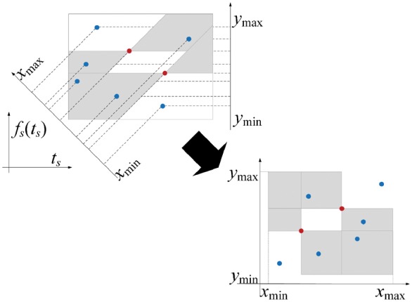
Identification of AUC-relevant positive-negative point pairs as a range query problem. The blue points denote elements of $\{(t_S,f_S(t_S))|S\in \mathcal{P}\}$, while the red points denote elements of $\{(t_S,f_S(t_S))|S\in \mathcal{N}\}$. $x_{\min }$,$x_{\max }$, $y_{\min }$, and $y_{\max }$ are defined in (21). After the bijective map of these points into another 2-d space, for each red point, there are two corresponding axis-parallel shadowed rectangles (defined in (21)) with it as one of the vertices, only those positive (blue) points which lie inside the rectangles need to be considered

Problem 2. Given a 2-dimensional point set ${\mathcal{Z}}_{\mathcal{P}}=\{(x_S,y_S)|S\in \mathcal{P}\}$, report the elements of ${\mathcal{Z}}_{\mathcal{P}}$ that lie in a specific rectangle (specifically, $[x_{\min },x_{S_2}]\times [y_{S_2},y_{\max }]$ or $[x_{S_2},x_{\max }]\times [y_{\min },y_{S_2}]$), where

$$\begin{array}{c}{x}_{\max }=\underset{S\in \mathcal{P}}{\max }{x}_S,\mathrm{ }{x}_{\min }=\underset{S\in \mathcal{P}}{\min }{x}_S,\\ y_{\max }=\underset{S\in \mathcal{P}}{\max }{y}_S,\mathrm{ }{y}_{\min }=\underset{S\in \mathcal{P}}{\min }{y}_S.\end{array}$$ (21)

The key observation here is that Problem 2 is a special case of the orthogonal range search, a well-studied problem in the computational geometry community and many specialized efficient algorithms have been developed for it (Agarwal and Erickson, 1999). As is in our case, range search typically has to deal with a large number of similar queries on the same dataset, so it is worthwhile to firstly pre-organize the queried dataset into a data structure that can efficiently answer many potential queries by exploiting their shared geometric properties.

In CDAUC, we specifically adopt the 2-d range tree for processing ${\mathcal{Z}}_{\mathcal{P}}$, which can achieve faster answer times than alternative data structures (e.g. k-d tree) by using more storage space (Agarwal and Erickson, 1999). Roughly speaking, the 2-d range tree is a two-level balanced search tree (BST) recursively defined over each dimension of the input point set (see Fig. 4 for an illustrative example). By adopting the ‘Fractional Cascading’ technique, the query time of range tree can be further reduced. We refer the reader to (De Berg et al., 2000) for details on related construction and query protocols.

Fig. 4.

Illustration of a range tree for storing eight points, including (1,5), (3,8), (4,2), etc. The first level is a BST defined on the first coordinate (colored in red). Each vertex v of this tree stores a BST defined on the second coordinate (colored in blue) of the points in the subtree of v. For example, in BST defined on the first coordinate, the subtree of node ‘4’ contains two points: (9,4) and (6,7), therefore this node would store a BST constructed according to the second coordinate of these two points

The overall process of identifying Ξ using range tree is presented in Algorithm 3. Note that the construction of range tree requires that there should be no duplicate points in ${\mathcal{Z}}_{\mathcal{P}}$(De Berg et al., 2000). Thus, we have to firstly preprocess ${\mathcal{Z}}_{\mathcal{P}}$ to obtain $\widehat{{\mathcal{Z}}_{\mathcal{P}}}$ such that this requirement could be fulfilled (line 2). Since each element of $\widehat{{\mathcal{Z}}_{\mathcal{P}}}$ could represent multiple elements of the original ${\mathcal{Z}}_{\mathcal{P}}$, it is necessary to additionally record the number of occurrences of each element of $\widehat{{\mathcal{Z}}_{\mathcal{P}}}$ in ${\mathcal{Z}}_{\mathcal{P}}$.

As is analyzed in Supplementary Material S4, the overall complexity of Algorithm 3 is $O(2\left|\mathcal{P}\right|\hspace{0.17em}\text{log}\hspace{0.17em}(\left|\mathcal{P}\right|)+2\left|\mathcal{N}\right|\hspace{0.17em}\text{log}\hspace{0.17em}(\left|\mathcal{P}\right|)+\left|\mathcal{X}\right|)$, which could be much faster than the aforementioned brute-force implementation if $\left|\mathcal{X}\right|$ is significantly smaller than $\left|\mathcal{P}\right|\cdot \left|\mathcal{N}\right|$. The efficiency of CDAUC will be experimentally demonstrated in Section 4.3.

Algorithm 3.

Range-tree-based implementation of line 1 of Algorithm 2

Input: Positive set $\mathcal{P}$, negative set $\mathcal{N}$, current solution $w^{k,i}$.

Output: The set χ.

1.   Use (19) to calculate ${\mathcal{Z}}_{\mathcal{P}}=\{(x_{S_1},y_{S_1})|S_1\in \mathcal{P}\}$ and ${\mathcal{Z}}_{\mathcal{N}}=\{(x_{S_2},y_{S_2})|S_2\in \mathcal{N}\}$.

2.   Create a new set $\widehat{{\mathcal{Z}}_{\mathcal{P}}}$ which stores the unique elements of ${\mathcal{Z}}_{\mathcal{P}}$.

3.    Construct the range tree for $\widehat{{\mathcal{Z}}_{\mathcal{P}}}$.

4.    for all $(x_{S_2},y_{S_2})\in {\mathcal{Z}}_{\mathcal{N}}$do

5.    Use the constructed range tree to identify ${\mathcal{Y}}_{S_2}^1$ and ${\mathcal{Y}}_{S_2}^2$ based on (21).

6.    Traverse ${\mathcal{Y}}_{S_2}^1$ and ${\mathcal{Y}}_{S_2}^2$ and screen out the elements of ${\mathcal{Y}}_{S_2}^3$.

7.    end for

8.    Calculate χ using (17).

9.    Return χ.

3.6.2 Parameter setting

Recall that CDAUC has a pair of hyper-parameters $(t_l,t_r)$, which determines the search interval of each sub-problem (10). Since the analysis in previous subsections establishes that ${\ell }_t(t)$ is piecewise constant, if we can choose $(t_l,t_r)$ properly such that ${\ell }_t(t)$ is constant when $t>t_r$ and $t<t_l$, then the optimal t that globally maximizes ${\ell }_t(t)$ could be obtained by solving (10). In the Supplementary Material S5, we show that $(t_l,t_r)$ which satisfies this requirement can be efficiently found in $O(\left|\mathcal{P}\right|+\left|\mathcal{N}\right|)$ time.

3.6.3 Parallelization

By examining Algorithm 1, it is easy to see that in each outer iteration, the optimization problem (10) for every $1\le i\le 4l$ is solved independently, thus CDAUC can be parallelized simply by distributing these sub-problems to different threads.

4 Results

In this section, the performance of CDAUC is systematically evaluated. As one of the most widely used DML methods, DREME was firstly adopted to identify the preliminary motifs, these motifs were then re-optimized by CDAUC and DIMO separately. The outputs of three methods were then compared to assess CDAUC for optimizing DML motifs. In addition, we also adopted HOMER as a comparison baseline.

We downloaded the ChIP-seq data for 43 TFs in K562 cell line from ENCODE. As in (Patel and Stormo, 2014), for each TF, 1000 peaks in the length of 100–500 base pairs with the highest significance score were collected as the positive set. On the other hand, the choice of negative sequences can significantly affect the results of DML methods (Maaskola and Rajewsky, 2014), for example, if we simply choose intergenic regions that do not overlap with any peaks as the negative set, the resultant motifs could be highly GC-rich, reflecting the general preference for GC-rich regions of some TFs. In this paper, we firstly followed (Orenstein and Shamir, 2014; Setty and Leslie, 2015; Wang et al., 2012; Yao et al., 2013) and obtained a background sequence for each peak by randomly choosing a sequence of the same length and lies 0–200 nt from the edge on either up or down strand.

4.1 Cross validation

Evaluations of different models for motif discovery in ChIP-seq data are generally difficult, as the ground-truth motif instances are typically not known. Following (Agostini et al., 2014; Patel and Stormo, 2014; Siebert and Seding, 2016; Simcha et al., 2012), to quantitatively evaluate CDAUC, we adopted the ‘reference-free’ cross-validation strategy. In other words, for each TF we took the corresponding set of positive/negative sequences and partitioned them into three sets (‘folds’) of roughly equal size, for each fold, a PWM was learned on the other folds and then evaluated on the fold. We compared the 3-fold cross-validated average AUCs of three methods on 43 collected datasets. Table 1 shows that in all cases, our approach performed better than the other three methods.

Table 1.

Cross-validated AUC comparison of various methods on 43 datasets

TF	DREME	DIMO	HOMER	CDAUC	TF	DREME	DIMO	HOMER	CDAUC	TF	DREME	DIMO	HOMER	CDAUC
ARID3	0.650	0.706	0.666	0.734	JUND	0.909	0.920	0.908	0.941	BLR1	0.555	0.615	0.624	0.704
ATF1	0.760	0.838	0.791	0.869	KAP1	0.603	0.633	0.592	0.665	BLR1NB	0.700	0.751	0.720	0.780
BACH1	0.882	0.901	0.880	0.940	MAFF	0.858	0.886	0.841	0.896	TBP	0.616	0.628	0.594	0.652
CCNT2	0.636	0.715	0.679	0.780	MAFK	0.889	0.906	0.885	0.917	TFIIB	0.678	0.691	0.695	0.717
CDPSC	0.775	0.824	0.801	0.841	MAX	0.815	0.863	0.798	0.870	TFIIF	0.702	0.714	0.668	0.725
CEBPB	0.836	0.931	0.842	0.945	MAZ	0.740	0.750	0.746	0.770	UBF	0.716	0.727	0.713	0.744
CHD2	0.794	0.873	0.777	0.886	MXI1	0.653	0.705	0.677	0.726	UBT	0.689	0.704	0.710	0.737
CMYC	0.706	0.797	0.731	0.827	NFYA	0.931	0.944	0.934	0.959	USF2	0.964	0.970	0.931	0.974
CORESTAB	0.690	0.758	0.716	0.774	NFYB	0.922	0.947	0.847	0.948	ZC3	0.665	0.683	0.681	0.720
CORESTSC	0.670	0.712	0.693	0.727	NRF1	0.929	0.962	0.951	0.967	ZNF143	0.617	0.686	0.592	0.752
CTCFB	0.781	0.801	0.792	0.811	P300	0.776	0.817	0.788	0.832	ZNF27	0.557	0.617	0.559	0.662
DEC1	0.830	0.885	0.841	0.894	P300SC	0.781	0.825	0.788	0.836	ZNF384	0.854	0.856	0.781	0.858
ELK1	0.885	0.899	0.832	0.912	RFX5	0.623	0.636	0.617	0.679	ZNFMIZ	0.753	0.789	0.753	0.811
HCFC1	0.607	0.773	0.637	0.805	SMC3	0.817	0.843	0.831	0.855
HMGN3	0.708	0.716	0.694	0.738	TAL1	0.798	0.868	0.797	0.883

When the ground truth motif is not known, an alternative metric for assessing elicited motifs would be Centrimo P-value, which measures the motif enrichment in central regions of the detected peaks (Bailey and Machanick, 2012). Evaluations based on this metric similarly show that CDAUC outperforms other compared methods (Supplementary Table S1).

To better illustrate the behavior of CDAUC, in Table 2 we also visually present the differences between the original DREME motif and motifs optimized using CDAUC for three TFs, which show that the quality of motifs is improved mainly by changing preferred bases of PWMs.

Table 2.

Visual comparison of motifs between the DREME and CDAUC

4.2 Alternative choice of the negative set

Although experimental results in the previous subsection demonstrate the advantages of CDAUC, flanking sequence is merely one consideration of background set when finding motifs in ChIP-seq datasets. In this section, we consider another widely used strategy for constructing the negative data, which is to artificially generate sequences by mimicking the positive data (Bailey, 2011; Grau et al., 2013; Maaskola and Rajewsky, 2014; Tanaka et al., 2014). Here, for each positive sequence, we used the ‘shuffle’ function of the HMMER package (Finn et al., 2011) to generate 50 negative sequences with the same 1st order Markov properties, and repeated the cross validation process. Meanwhile, as the data sets are highly imbalanced, we also adopted the area under the precision-recall curve (AUPRC) (Davis and Goadrich, 2006) as the additional evaluation metrics. The final results consistently show that CDAUC perform better than other methods (Supplementary Tables S2 and S3).

4.3 Computational efficiency

To evaluate the time complexity of the proposed method, CPU time required by different algorithms on the first four TFs are shown in Figure 5. The data discussed in Section 4.2 are chosen for time benchmarking due to their larger sizes. As the average computational time required by DREME on these datasets is 229 s, the results show that CDAUC is significantly faster than DIMO, demonstrating also that CDAUC could be practically used to improve the quality of motifs, without costing too much additional computational time.

Fig. 5.

Time comparison of DIMO and CDAUC by examining the training AUC as a function of the computational time

4.4 Refinements of PWMs inferred via CNNs

In this section, we use simulated data to evaluate the performance of CDAUC for refining CNN-generated PWMs. The advantage of synthetic data is that the ground-truth motifs are known is advance, which makes it easier to investigate the potential limitations of CNNs for identifying motifs.

4.4.1 Data preparation

For each time of simulation, we firstly sampled 10 000 intergenic genomic regions of length 500 as the positive set, then generated 10 000 negative sequences using second-order Markov models learned from the positive sequences. We then constructed three motifs of length eight with a specific information content (IC) value using the ‘polarization’ technique discussed in (Maaskola and Rajewsky, 2014), these motifs were implanted into the positive sequences with probabilities of 90%, 80% and 70%, respectively. For each IC value, we performed five simulations and reported the average performances.

4.4.2 CNN model

We adopted the implementation discussed in (Zeng et al., 2016). We also directly used the hypermeter set mentioned there, and randomly sampled 1/4 of the data as the validation set for determining hyperparameters. As is suggested in (Alipanahi et al., 2015), we set the number of PWMs and the PWM width both as 10, such that they are larger than the ground-truth value and may thereby prevent the training process from getting trapped at poor local minima.

4.4.3 Evaluation protocol

The PWMs were firstly learned using CNNs, then re-optimized using DIMO and CDAUC, respectively. The outputs of three methods were then compared. Following (Kilpatrick et al., 2014; Maaskola and Rajewsky, 2014), we quantify the performance for predicting the motif positions using nucleotide-level Matthews correlation coefficient (nCC) and site-level average precision (sAP). As there are more PWMs than the true motifs, the performance for predicting each motif is measured by taking the maximum over the performance of all PWMs. Formal descriptions of such an evaluation protocol are presented in Supplementary Material S6.

The average performances of three methods for predicting the underlying motifs are presented in Table 3. The results show that as IC value decreases, the performance of CNN degrades rapidly. This is expected, as degenerate motifs may generate more diverse site sequences and thereby more easily mislead the CNNs. While this problem cannot be completely solved by CDAUC, the results still show that in all cases, it managed to significantly improve the similarities of CNN PWMs to the ground-truth motifs.

Table 3.

Comparisons of various methods for predicting motif positions

Metric	IC	CNN	DIMO	CDAUC
nCC	4	0.027	0.060	0.082
	8	0.117	0.234	0.331
	16	0.592	0.799	0.897
sAP	4	0.067	0.109	0.136
	8	0.160	0.274	0.369
	16	0.661	0.903	0.964

The best performance achieved by all evaluated methods are highlighted in bold.

5 Conclusion

In this paper, we propose a novel algorithm called CDAUC for optimizing DML-learned motifs based on the area under the receiver-operating characteristic curve (AUC) criterion, which has been widely used in the literature to evaluate the accuracy of extracted motifs. Experimental results on real world high-throughput datasets illustrate the performance of the proposed algorithm for refining motifs learned by DML methods.

Meanwhile, as the recently proposed CNN-based methods seem to solve a very similar problem of discriminating two sets of sequences, we also attempt to clarify the difference between CNNs and DMLs. The analysis in Section 2 and the experimental result in Section 4.4 collectively suggest that it may be problematic to view CNNs as motif learning methods that perform the same task as DMLs. Meanwhile, DMLs may even be helpful for improving the interpretability of CNNs. While this limitation of CNNs has (to our best knowledge) not been noted in the literature before, similar problems have been observed for other methods that also attempt to infer the collective effect of multiple features on the TF binding. For example, in k-mer-based SVM models, there can be a large number of very similar k-mer features that are all significant for the prediction task (Ghandi et al., 2014). To deal with such difficulties, SeqGL (Setty and Leslie, 2015) and MIL (Gao and Ruan, 2017) similarly adopt a DML method (HOMER) to interpret their outputs, while gkmSVM (Ghandi et al., 2014) would cluster k-mers into PWMs for further analysis, which could be viewed as a simplified version of motif learning methods such as (Liu et al., 2016).

There are several directions in which we intend to extend this work. Firstly, although PWM is the most commonly used model for sequence motifs, there is growing evidence that more advanced models can significantly outperform PWM (Siebert and Seding, 2016), it would be interesting to investigate AUC optimization of these advanced models.

Secondly, it is also important to note that AUC is not necessarily the most appropriate objective function for certain types of DML problems. For example, the AUPRC adopted in Section 4.2 may be a more informative metric for highly skewed data (He and Garcia, 2009; Kelley et al., 2016). It would thus be useful to extend CDAUC to optimize other important metrics such as AUPRC.

Finally, as in this paper we focus on DML-related motif optimization problems, the studies related to CNNs are only preliminary, and we plan to more thoroughly explore the pros and cons of CNNs and DMLs in future works.

References

- Agarwal P.K., Erickson J. (1999) Geometric range searching and its relatives. Contemp. Math., 223, 1–56. [Google Scholar]
- Agostini F. et al. (2014) SeAMotE: a method for high-throughput motif discovery in nucleic acid sequences. BMC Genomics, 15, 925. [DOI] [PMC free article] [PubMed] [Google Scholar]
- Alipanahi B. et al. (2015) Predicting the sequence specificities of DNA- and RNA-binding proteins by deep learning. Nat. Biotechnol., 33, 831–838. [DOI] [PubMed] [Google Scholar]
- Bailey T.L. (2011) DREME: motif discovery in transcription factor ChIP-seq data. Bioinformatics, 27, 1653–1659. [DOI] [PMC free article] [PubMed] [Google Scholar]
- Bailey T.L., Machanick P. (2012) Inferring direct DNA binding from ChIP-seq. Nucleic Acids Res., 40, 10. [DOI] [PMC free article] [PubMed] [Google Scholar]
- Davis J., Goadrich M. (2006) The relationship between Precision-Recall and ROC curves. ICML. Association for Computing Machinery, pp. 233–240. [Google Scholar]
- De Berg M. et al. (2000) Computational geometry. Springer Berlin Heidelberg. [Google Scholar]
- Dror I. et al. (2015) A widespread role of the motif environment in transcription factor binding across diverse protein families. Genome Res., 25, 1268–1280. [DOI] [PMC free article] [PubMed] [Google Scholar]
- Finn R.D. et al. (2011) HMMER web server: interactive sequence similarity searching. Nucleic Acids Res, 39, W29–W37. [DOI] [PMC free article] [PubMed] [Google Scholar]
- Gao W. et al. (2016) One-pass AUC optimization. Artif. Intell., 236, 1–29. [Google Scholar]
- Gao Z., Ruan J. (2017) Computational modeling of in vivo and in vitro protein-DNA interactions by multiple instance learning. Bioinformatics, doi: 10.1093/bioinformatics/btx115. [DOI] [PMC free article] [PubMed] [Google Scholar]
- Ghandi M. et al. (2014) Enhanced regulatory sequence prediction using gapped k-mer features. PLoS Comput. Biol., 10, 15. [DOI] [PMC free article] [PubMed] [Google Scholar]
- Grau J. et al. (2013) A general approach for discriminative de novo motif discovery from high-throughput data. Nucleic Acids Res., 41, 11. [DOI] [PMC free article] [PubMed] [Google Scholar]
- He H., Garcia E.A. (2009) Learning from Imbalanced Data. IEEE Trans. Knowledge Data Eng., 21, 1263–1284. [Google Scholar]
- Heinz S. et al. (2010) Simple combinations of lineage-determining transcription factors prime cis-regulatory elements required for macrophage and B cell identities. Mol. Cell., 38, 576–589. [DOI] [PMC free article] [PubMed] [Google Scholar]
- Hsieh C.-J., Dhillon I.S. (2011) Fast coordinate descent methods with variable selection for non-negative matrix factorization. KDD. Association for Computing Machinery, pp. 1064–1072. USA. [Google Scholar]
- Ikebata H., Yoshida R. (2015) Repulsive parallel MCMC algorithm for discovering diverse motifs from large sequence sets. Bioinformatics, 31, 1561–1568. [DOI] [PMC free article] [PubMed] [Google Scholar]
- Kelley D.R. et al. (2016) Basset: learning the regulatory code of the accessible genome with deep convolutional neural networks. Genome Res., 26, 990–999. [DOI] [PMC free article] [PubMed] [Google Scholar]
- Kilpatrick A.M. et al. (2014) Stochastic EM-based TFBS motif discovery with MITSU. Bioinformatics, 30, i310–i318. [DOI] [PMC free article] [PubMed] [Google Scholar]
- Lesluyes T. et al. (2014) Differential motif enrichment analysis of paired ChIP-seq experiments. BMC Genomics, 15, 1–13. [DOI] [PMC free article] [PubMed] [Google Scholar]
- Li L. et al. (2007) GAPWM: a genetic algorithm method for optimizing a position weight matrix. Bioinformatics, 23, 1188–1194. [DOI] [PubMed] [Google Scholar]
- Liu H. et al. (2016) Fast motif discovery in short sequences. ICDE. IEEE, Piscataway, NJ, USA, pp. 1158–1169. [Google Scholar]
- Maaskola J., Rajewsky N. (2014) Binding site discovery from nucleic acid sequences by discriminative learning of hidden Markov models. Nucleic Acids Res., 42, 12995–13011. [DOI] [PMC free article] [PubMed] [Google Scholar]
- Mason M.J. et al. (2010) Identification of Context-Dependent Motifs by Contrasting ChIP Binding Data. Bioinformatics, 26, 2826–2832. [DOI] [PMC free article] [PubMed] [Google Scholar]
- McLeay R.C., Bailey T.L. (2010) Motif enrichment analysis: a unified framework and an evaluation on ChIP data. BMC Bioinformatics, 11, 165. [DOI] [PMC free article] [PubMed] [Google Scholar]
- Narasimhan H., Agarwal S. (2013) A structural SVM based approach for optimizing partial AUC. ICML. International Machine Learning Society (IMLS), pp. 516–524. New York, USA. [Google Scholar]
- Orenstein Y., Shamir R. (2014) A comparative analysis of transcription factor binding models learned from PBM, HT-SELEX and ChIP data. Nucleic Acids Res., 42, 10. [DOI] [PMC free article] [PubMed] [Google Scholar]
- Patel R.Y., Stormo G.D. (2014) Discriminative motif optimization based on perceptron training. Bioinformatics, 30, 941–948. [DOI] [PMC free article] [PubMed] [Google Scholar]
- Setty M., Leslie C.S. (2015) SeqGL identifies context-dependent binding signals in genome-wide regulatory element maps. PLoS Comput. Biol., 11, 21.. [DOI] [PMC free article] [PubMed] [Google Scholar]
- Siebert M., Seding J. (2016) Bayesian Markov models consistently outperform PWMs at predicting motifs in nucleotide sequences. Nucleic Acids Res., 44, 6055–6069. [DOI] [PMC free article] [PubMed] [Google Scholar]
- Simcha D. et al. (2012) The limits of de novo DNA motif discovery. PLoS One, 7, 9. [DOI] [PMC free article] [PubMed] [Google Scholar]
- Tanaka E. et al. (2014) Improving MEME via a two-tiered significance analysis. Bioinformatics, 30, 1965–1973. [DOI] [PMC free article] [PubMed] [Google Scholar]
- Valen E. et al. (2009) Discovery of regulatory elements is improved by a discriminatory approach. PLoS Comput. Biol., 5, 8. [DOI] [PMC free article] [PubMed] [Google Scholar]
- Wang J. et al. (2012) Sequence features and chromatin structure around the genomic regions bound by 119 human transcription factors. Genome Res., 22, 1798–1812. [DOI] [PMC free article] [PubMed] [Google Scholar]
- Weirauch M.T. et al. (2013) Evaluation of methods for modeling transcription factor sequence specificity. Nat. Biotechnol., 31, 126–134. [DOI] [PMC free article] [PubMed] [Google Scholar]
- Yao Z. et al. (2013) Discriminative motif analysis of high-throughput dataset. Bioinformatics, 30, 775–783. [DOI] [PMC free article] [PubMed] [Google Scholar]
- Zeng H.Y. et al. (2016) Convolutional neural network architectures for predicting DNA-protein binding. Bioinformatics, 32, 121–127. [DOI] [PMC free article] [PubMed] [Google Scholar]
Associated Data
This section collects any data citations, data availability statements, or supplementary materials included in this article.