SparseIso: a novel Bayesian approach to identify alternatively spliced isoforms from RNA-seq data

Abstract

Motivation

Recent advances in high-throughput RNA sequencing (RNA-seq) technologies have made it possible to reconstruct the full transcriptome of various types of cells. It is important to accurately assemble transcripts or identify isoforms for an improved understanding of molecular mechanisms in biological systems.

Results

We have developed a novel Bayesian method, SparseIso, to reliably identify spliced isoforms from RNA-seq data. A spike-and-slab prior is incorporated into the Bayesian model to enforce the sparsity for isoform identification, effectively alleviating the problem of overfitting. A Gibbs sampling procedure is further developed to simultaneously identify and quantify transcripts from RNA-seq data. With the sampling approach, SparseIso estimates the joint distribution of all candidate transcripts, resulting in a significantly improved performance in detecting lowly expressed transcripts and multiple expressed isoforms of genes. Both simulation study and real data analysis have demonstrated that the proposed SparseIso method significantly outperforms existing methods for improved transcript assembly and isoform identification.

Availability and implementation

The SparseIso package is available at http://github.com/henryxushi/SparseIso.

Supplementary information

Supplementary data are available at Bioinformatics online.

1 Introduction

Recent studies have shown that more than 90% of the human genes undergo the alternative splicing to give rise to different mRNA and protein isoforms (Wang et al., 2008). The pervasive alternative splicing events allow genes to produce variant proteins functioning in different modules, contributing to the complexity of biological systems. It is crucial to study the transcriptome structure for understanding the regulation mechanisms in cells. RNA sequencing (RNA-seq) technology has revolutionized the transcriptomic study by deep sampling the transcriptome with tens to hundreds of millions of short reads. The massive short reads make it possible to detect splice junctions covered by the reads. To analyze RNA-seq data, short reads are usually first aligned to a reference genome by splice sequence aligners such as STAR (Dobin et al., 2013) and TopHat2 (Kim et al., 2013). The aligners specifically developed for RNA-seq data can also identify splice junctions by a spliced-mapping of short reads, which offers the opportunity to infer the structure of isoforms.

In recent years, several computational methods have been developed to detect and quantify isoforms using aligned RNA-seq data. These algorithms usually start with building splicing graphs by identifying exons and splice junctions from short reads. In a splicing graph, two exons will be connected if the connection is supported by spliced reads. One way to identify the expressed isoforms is to enumerate all possible maximal paths of a splicing graph to find candidate isoforms (Guttman et al., 2010). Due to the large noise and mapping uncertainty existed in RNA-seq data, the isoforms enumerated are likely with a high rate of false positives. To tackle this problem, the idea of ‘sparsity’ has been incorporated to infer the expressed isoforms without overfitting the observed reads. Cufflinks (Trapnell et al., 2010) tries first to assemble the short reads to scaffolds and then build an overlap graph based on the scaffolds. The percent-splice-in (PSI) information is then calculated at each candidate junction. The sparsity constraint is implicitly incorporated by searching for a minimum set of paths that can explain the PSIs. It is an effective way to reduce false positives by searching for a minimum set of paths; however, it adversely elicits Cufflinks to miss many truly expressed isoforms, increasing the false negative rate significantly. Several regularization algorithms have also been developed to address the same overfitting problem. IsoLasso (Li et al., 2011) and iReckon (Mezlini et al., 2013) formulate the problem as a linear regression problem. The read coverage at each exon is modeled as a mixture of abundances of multiple isoforms. A regularization term is added to penalize the abundances of isoforms to enforce sparsity. CEM (Li and Jiang, 2012) is developed to address the effect of dispersed read counts observed from RNA-seq data. By using a Dirichlet prior, CEM penalizes on the relative abundances of isoforms. The optimal solution is achieved by an expectation-maximization (EM) elimination algorithm. All these regularization-based methods solve the mixture problem by thresholding (or discarding) the isoforms of low abundance, leaving those truly expressed isoforms (although of low abundance) unidentified. Furthermore, the optimal value of the regularization parameter is often intractable. Different parameter settings would give rise to different results, affecting the generalization of a regularization-based method when applied to various datasets. Moreover, current regularization-based methods only have point estimation of the isoform expressions. Due to the large noise of RNA-seq data, interval estimation gains more confidence for abundance quantification. Recently, a probabilistic approach called Bayesembler (Maretty et al., 2014) is developed to address the concerns about the thresholding-based approaches. Bayesembler uses a generative model to model the sequencing generation process. By using a Gibbs sampling strategy, the confidence level of the isoform abundance can be estimated. Bayesembler strictly defines the false isoforms as zero abundance isoforms; then all aligned reads will be assigned only to predicted isoforms. However, the sequence error and the mapping uncertainty could make the confidence level of noisy isoforms overestimated.

In this paper, we develop a new Bayesian method, SparseIso, to identify isoforms from RNA-seq data. We first employ a similar strategy used in IsoLasso and Bayesembler to build splicing graphs. To account for the overdispersion observed in RNA-seq data, we use a negative binomial (NB) model to model the read counts. The expressions of exons or junctions are modeled as mixtures of expressions of individual isoforms. We use a spike-and-slab prior to help categorize the expression state of candidate isoforms into expressed and unexpressed groups. The actual abundance of isoform expression is modeled based on the expression state, where the abundance of isoforms in the unexpressed group will be restricted to be close to zero. Different from Bayesembler, we allow the false isoforms to have small abundance, which may help lower the confidence of candidate isoforms caused by the error. The expression state assignment is modeled as a Bernoulli process with a higher probability for the unexpressed group than the expressed group, which contributes to the spikes at zero in the prior distribution. The spikes at zero will help enforce sparsity in Bayesian estimation of expressed isoforms. By using a Gibbs sampling strategy, we iteratively estimate the expression state of an isoform and its actual abundance. The final identified set of isoforms consists of the ones with high confidence levels.

2 Materials and methods

The flowchart of the proposed SparseIso method is shown in Figure 1. The algorithm starts with RNA-seq data aligned by splice aligners such as TopHat2. We use a similar strategy used in IsoLasso and Bayesembler to construct the splicing graph and enumerate the candidate isoforms. For each exon and splice junction identified in the graph, we use a negative binomial (NB) model to model the read counts and segment coverage. The segment coverage is then modeled as a mixture of isoform abundances. We use a spike-and-slab prior distribution to model the isoform abundance. By using a binary variable to indicate the expression state of isoforms, the candidate isoforms can be categorized into expressed and unexpressed groups. The variance of the isoform abundance is controlled by the expressed state. The abundance of an unexpressed isoform will have very low variation around 0, while the expressed isoforms can have higher abundances with higher variation. To infer the parameters of the Bayesian model, we apply a Gibbs sampling strategy to estimate the joint posterior distribution. Finally, we estimate the confidence level of isoforms as the frequency of selection. The final set of isoforms is selected from the isoforms that have the confidence level greater than 0.5. The abundance of the identified isoforms can also be estimated by samples drawn from the corresponding posterior distribution. The dependency of the random variables used in the Bayesian model is shown in Figure 2; more details about the model variables will be described in the following sections.

Fig. 1.

Overview of the proposed SparseIso approach. SparseIso consists of the following steps: (1) splicing graph construction; (2) sampling of isoform existence; (3) sampling of isoform abundance

Fig. 2.

The dependency graph of the model parameters of SparseIso. The unshaded and shaded circles indicate the unobserved and observed random variables, respectively. The unobserved random variables need to be estimated from the Gibbs sampling approach. The arrows indicate the dependencies between random variables and parameters

2.1 Candidate transcript construction

The sequence reads are first aligned to the reference genome by RNA-seq aligners such as TopHat2. We use the program ‘processsam’ in the CEM package (Li and Jiang, 2012) to identify exon regions, intron regions and junctions. Different from traditional splicing graphs, splice junctions are also included in the node set of the graph. A more detailed description of candidate transcript construction can be found in Supplementary Section S1.1. All maximal paths starting from TSS nodes and ending with TES nodes are enumerated from the graph by a depth-first search.

2.2 Read count model

In RNA-seq experiments, the reads generated can be modeled as a sampling process from the transcriptome. If we assume a uniform sampling process, the reads can be modeled by a binomial model. Poisson distribution is widely used to approximate the binomial model (Jiang and Wong, 2009) when the number of reads is huge. Due to the sequencing and positional bias of RNA-seq data, the reads are likely not sampled uniformly from the transcriptome (Hansen et al., 2010; Li and Jiang, 2012; Mortazavi et al., 2008). The observed over-dispersion pattern of the read count distribution violates the assumption of Poisson distribution. Thus, a two-parameter model, NB model, is used to account for the bias in RNA-seq data. As unique splice junction is the key characteristic of isoforms, quantification of splice junctions would help resolve the isoform interpretation better. In our model, we also include splice junctions in the exon set to model the spliced reads. We define the segment as the union set of exons and splice junctions.

For segment $i$ identified from the data, its read count${\mathrm{ }\mathrm{y}}_{\mathrm{i}}$ follows an NB distribution as follows:

$$y_i\mathrm{ }\sim \mathrm{ }\mathrm{N}\mathrm{B}\left(B_i{l}_i/{\tau }_i^2,{\tau }_i^2/({\tau }_i^2+1)\right),$$ (1)

with mean ${\mathrm{B}}_i{l}_i$ and variance$\mathrm{ }{\mathrm{B}}_i{l}_i(1+{\mathrm{\tau }}_i^2)$. ${\mathrm{B}}_i$ is the expression level of the segment indicating the average number of reads sampled at each base of segment $i$. $l_i$ is the effective length of the segment representing the expected number of start sites having reads mapped within the segment, which is widely used for transcript quantification with RNA-seq data (Li and Dewey, 2011; Trapnell et al., 2010). The parameter ${\tau }_i^2$ controls the degree of over-dispersion at segment$\mathrm{ }i$. If$\mathrm{ }{\tau }_i^2\mathrm{ }$is close to 0, the NB distribution will approach to Poisson distribution. The NB model is equivalent to Poisson model assuming that the sampling probability follows a Gamma distribution (see Supplementary Section S1.2 for more details). A maximum likelihood estimator can be used to estimate $B_i$ and ${\tau }_i^2$ for each segment as described in (Piegorsch, 1990).

We use the same strategy as introduced in the count model of IsoLasso and CEM to count the reads for both single-end and paired-end data, knowing that the reads on segments are coming from different transcripts. When dealing with single-end data, we include splice junctions in the graph to further categorize reads. We use different strategies to process single-end and paired-end data. For single-end data, the segment count is the number of reads mapped entirely within the segment. The effective length is calculated as the number of starting bases that a read can be mapped within the segment. For paired-end data, the fragment length information can help further resolve the ambiguity in read assignment (see Supplementary Section S1.3 for more details). The fragment length distribution can be empirically estimated as a Gaussian distribution from the genes that only have a single path in the data (Roberts et al., 2011). Based on the fragment alignments, we enumerate ‘paired-end modules’ from the data. Each paired-end module consists of two segments that have paired fragment support. A paired-end module$,\mathrm{ }\mathrm{M}=\left({\mathrm{s}}_1,{\mathrm{s}}_2\right),$ is regarded as valid if we can find at least one fragment with one end mapped to segment ${\mathrm{s}}_1$ and the other end mapped to segment$\mathrm{ }{\mathrm{s}}_2$. The effective length of a paired-end module is the expected number of starting sites supporting the fragment alignment. For each possible read alignment at$\mathrm{ }{\mathrm{s}}_1$, we calculate the probability of a paired-end alignment at ${\mathrm{s}}_2$ based on estimated fragment length distribution. Let ${\mathrm{l}}_{\mathrm{M}}$ be the effective length of a paired-end module$\mathrm{ }\mathrm{M}$. ${\mathrm{l}}_{\mathrm{M}}$ can be calculated as follows:

$${\mathrm{l}}_{\mathrm{M}}={\sum }_{\mathrm{i}=1}^{{\mathrm{l}}_{\mathrm{s}1}}\mathrm{\Phi }\left({\mathrm{l}}_{\mathrm{i}}^{\mathrm{m}\mathrm{a}\mathrm{x}};{\mathrm{\mu }}_{\mathrm{l}},{\mathrm{\sigma }}_{\mathrm{l}}^2\right)-\mathrm{\Phi }({\mathrm{l}}_{\mathrm{i}}^{\mathrm{m}\mathrm{i}\mathrm{n}}-1;{\mathrm{\mu }}_{\mathrm{l}},{\mathrm{\sigma }}_{\mathrm{l}}^2).$$ (2)

Here, $\mathrm{i}$ is the starting position at ${\mathrm{s}}_1$, ${\mathrm{l}}_{\mathrm{s}1}$ is the effective length of ${\mathrm{s}}_1$, $\mathrm{\Phi }(\mathrm{x};{\mathrm{\mu }}_{\mathrm{l}},{\mathrm{\sigma }}_{\mathrm{l}}^2)$ is the cumulative distribution function of a normal distribution with mean ${\mathrm{\mu }}_{\mathrm{l}}$ and variance ${\mathrm{\sigma }}_{\mathrm{l}}^2$ (which can be estimated from the fragment length distribution). ${\mathrm{l}}_{\mathrm{i}}^{\mathrm{m}\mathrm{a}\mathrm{x}}$ and ${\mathrm{l}}_{\mathrm{i}}^{\mathrm{m}\mathrm{i}\mathrm{n}}$ are the maximum and minimum possible fragment lengths, respectively, where the starting point is $\mathrm{i}$ at ${\mathrm{s}}_1$ (see Supplementary Section S1.4 for more details). By using the paired-end module, we can better assign those uncertain reads on segments to candidate transcripts. We also use the NB model described above to model the count of a paired-end module. For the convenience of explanation, we simply call a paired-end module as a segment in the following context.

2.3 Mixture of reads from multiple transcripts

Similar to the segment read count, the number of reads generated from transcript $\mathrm{t}$ at segment $\mathrm{i}$ also follows an NB distribution:

$$y_{i,t}\mathrm{ }\sim \mathrm{ }\mathrm{N}\mathrm{B}\left({\beta }_t{l}_i/{\tau }_i^2,{\tau }_i^2/({\tau }_i^2+1)\right),$$ (3)

where ${\mathrm{\beta }}_{\mathrm{t}}$ is the expression level of isoform $\mathrm{t}$. The isoform structure enumerated from the splicing graph can be represented as a binary matrix $\mathrm{X}$ with size of $\mathrm{n}\hspace{0.17em}\times \hspace{0.17em}\mathrm{m}$, where $\mathrm{n}$ is the number of segments and $\mathrm{m}$ is the number of candidate isoforms. If isoform $\mathrm{t}$ has segment $\mathrm{i}$, $\mathrm{X}\left(\mathrm{i},\mathrm{ }\mathrm{t}\right)=1$; otherwise, $\mathrm{X}\left(\mathrm{i},\mathrm{ }\mathrm{t}\right)=0$. It is important to note that we can build $\mathrm{X}$ as a continuous-valued matrix instead of a binary matrix to model the positional dispersion over isoform (i.e. reads tend to be biased to the 3′ end) (Wu et al., 2011) (Roberts et al., 2011) (see Supplementary Section S1.5 for more details). Based on $\mathrm{X}$, the read counts observed at segment $\mathrm{i}$ can be considered as a mixture of reads from isoforms containing segment $\mathrm{i}$:

$${\mathrm{y}}_{\mathrm{i}}={\sum }_{\mathrm{t}=1}^{\mathrm{m}}\mathrm{X}\left(\mathrm{i},\mathrm{ }\mathrm{t}\right){\mathrm{y}}_{\mathrm{i},\mathrm{t}}\mathrm{ }\sim \mathrm{ }\mathrm{N}\mathrm{B}\left({\mathrm{l}}_{\mathrm{i}}({\sum }_{\mathrm{t}=1}^{\mathrm{m}}\mathrm{X}\left(\mathrm{i},\mathrm{t}\right){\mathrm{\beta }}_{\mathrm{t}})/{\mathrm{\tau }}_{\mathrm{i}}^2,{\tau }_i^2/({\tau }_i^2+1)\right).$$ (4)

As shown in (4), the mixture of reads from multiple transcripts is equivalent to a mixture of isoform abundances.

We assume the segment abundance follows a truncated normal distribution (with its mean being the linear mixture of isoform abundances):

$$\mathrm{B}|\mathrm{X},\mathrm{\beta }\sim {\mathrm{N}}_{+}\left(\mathrm{X}\mathrm{\beta },{\mathrm{\sigma }}^2{\mathrm{I}}_{\mathrm{n}}\right),$$ (5)

where $\mathrm{B}={\left[{\mathrm{B}}_1,\dots ,{\mathrm{B}}_{\mathrm{n}}\right]}^{\mathrm{T}}$, $\mathrm{\beta }={\left[{\mathrm{\beta }}_1,\dots ,{\mathrm{\beta }}_{\mathrm{m}}\right]}^{\mathrm{T}}$, ${\mathrm{I}}_{\mathrm{n}}$ is an identity matrix with size $\mathrm{n}$, and ${\mathrm{\sigma }}^2$ is the variance of noise. The prior distribution of ${\sigma }^2$ follows an inverse Gamma distribution. As the number of enumerated transcripts is much larger than the number of segments, it is necessary to enforce the sparsity in $\mathrm{\beta }$ to avoid the problem of over-fitting. In our model, we use a spike-and-slab prior (Ishwaran and Rao, 2005; Mitchell and Beauchamp, 1988) to model $\mathrm{\beta }$. We first introduce a binary variable $\mathrm{z}=[{\mathrm{z}}_1,{\mathrm{z}}_2,\dots ,{\mathrm{z}}_{\mathrm{m}}]$ indicating the existence of isoforms. $\mathrm{z}\mathrm{ }$can take two values ${\mathrm{z}}_0\mathrm{ }({\mathrm{z}}_0\ll 1)$ and $1$. If$\mathrm{ }{\mathrm{z}}_{\mathrm{t}}=1$, transcript $\mathrm{t}$ is expressed; otherwise, transcript $\mathrm{t}$ is not expressed. The distribution of $\mathrm{z}$ is a mixture of ${\mathrm{z}}_0$ and $1$:

$${\mathrm{z}}_{\mathrm{t}}\mathrm{ }\sim \mathrm{ }\mathrm{w}\mathrm{\delta }\left({\mathrm{z}}_{\mathrm{t}}-1\right)+\left(1-\mathrm{w}\right)\mathrm{\delta }\left({\mathrm{z}}_{\mathrm{t}}-{\mathrm{z}}_0\right),\mathrm{ }\mathrm{t}=1,\mathrm{ }2,\dots ,\mathrm{ }\mathrm{m},$$ (6)

where $\mathrm{\delta }\left(\mathrm{x}\right)=1$ when $\mathrm{x}\hspace{0.17em}=\hspace{0.17em}0$ and $\mathrm{\delta }\left(\mathrm{x}\right)=0$ when $\mathrm{x}\hspace{0.17em}\ne \hspace{0.17em}0$. $\mathrm{w}$ is the prior probability for an isoform to express. We let $\mathrm{w}$ follow a Beta distribution with shape parameters ${\mathrm{a}}_{\mathrm{w}}$ and ${\mathrm{b}}_{\mathrm{w}}$; $\mathrm{w}$ favors a small value to introduce the sparsity in the model.

Based on the expression state of isoform $\mathrm{z}$, we model $\mathrm{\beta }$ by a truncated normal distribution:

$${\mathrm{\beta }}_{\mathrm{t}}|{\mathrm{\gamma }}_{\mathrm{t}}^2,{\mathrm{z}}_{\mathrm{t}}\sim {\mathrm{N}}_{+}\left(0,{\mathrm{z}}_{\mathrm{t}}{\mathrm{\gamma }}_{\mathrm{t}}^2\right),\mathrm{ }\mathrm{t}=1,\mathrm{ }2,\dots ,\mathrm{ }\mathrm{m},$$ (7)

where ${\mathrm{N}}_{+}(0,{\mathrm{z}}_{\mathrm{t}}{\mathrm{\gamma }}_{\mathrm{t}}^2)$ is the truncated normal distribution with zero mean and variance of ${\mathrm{z}}_{\mathrm{t}}{\mathrm{\gamma }}_{\mathrm{t}}^2$, and ${\mathrm{\gamma }}^2=[{\mathrm{\gamma }}_1^2,{\mathrm{\gamma }}_2^2,\dots ,{\mathrm{\gamma }}_{\mathrm{m}}^2]$ is a parameter controlling the variability of isoform abundance. The prior distribution of ${\gamma }_t^2$ follows an inverse Gamma distribution. Note that modeling $\mathrm{\beta }$ by a normal distribution can guarantee the conjugacy of the model, as normal distribution is the conjugate prior distribution of a normal distribution with known variance. If ${\mathrm{z}}_{\mathrm{t}}={\mathrm{z}}_0$, the variance of ${\mathrm{\beta }}_{\mathrm{t}}$ is ${\mathrm{z}}_0{\mathrm{\gamma }}_{\mathrm{t}}^2$, which is very close to 0. As limited by the variance, isoform $\mathrm{t}$ is highly probable to be not expressed with abundance close to 0. If ${\mathrm{z}}_{\mathrm{t}}=1$, the variance of ${\mathrm{\beta }}_{\mathrm{t}}$ is ${\mathrm{\gamma }}_{\mathrm{t}}^2$, which can be a large value. In this case isoform $\mathrm{t}$ will be classified as expressed, as the abundance is more likely to be significantly larger than 0. With a small value of $\mathrm{w}$, the marginal distribution of $\mathrm{\beta }$ would have a high spike very close to 0 and another part (slab) larger than 0 (see Supplementary Fig. S1-3 for an example). Further details about the distributions of parameters in the model are provided in Supplementary Section S1-7.

2.4 Estimation of model parameters using Gibbs sampling

Due to the conjugacy of our prior model, we can use Gibbs sampling to estimate the model parameters given the candidate isoform structure $\mathrm{X}$ and estimated segment abundance$\mathrm{ }\mathrm{B}$. By sampling from the conditional distribution of the parameter set {$\mathrm{\beta },\mathrm{ }\mathrm{z},{\mathrm{\gamma }}^2,{\mathrm{\sigma }}^2,\mathrm{ }\mathrm{w}$}, we aim for an accurate inference of expressed isoforms $\mathrm{z}$ and corresponding abundance$\mathrm{ }\mathrm{\beta }$. The joint posterior distribution of all parameters can be factorized as follows:

$$\mathrm{p}\left(\mathrm{\beta },{\mathrm{\gamma }}^2,\mathrm{ }\mathrm{z},{\mathrm{\sigma }}^2,\mathrm{ }\mathrm{w}||\mathrm{X},\mathrm{B}\right)\sim \mathrm{p}\left(\mathrm{B}||\mathrm{X},\mathrm{\beta },{\mathrm{\sigma }}^2\right)\times \mathrm{p}\left(\mathrm{\beta }||{\mathrm{\gamma }}^2,\mathrm{ }\mathrm{z}\right)\times \mathrm{p}\left({\mathrm{\gamma }}^2\right)\times \mathrm{ }\mathrm{p}\left(\mathrm{z}||\mathrm{w}\right)\times \mathrm{p}\left(\mathrm{w}\right)\times \mathrm{p}\left({\mathrm{\sigma }}^2\right).$$ (8)

The conditional distribution of $\mathrm{\beta }$ follows a truncated normal distribution:

$$\mathrm{p}\left(\mathrm{\beta }\right|\mathrm{B},\mathrm{ }\mathrm{X},\mathrm{ }\mathrm{z},{\mathrm{\gamma }}^2,{\mathrm{\sigma }}^2)\mathrm{ }\sim \mathrm{ }{\mathrm{N}}_{+}\left({\mathrm{A}}^{-1}{\mathrm{X}}^{\mathrm{T}}\mathrm{B},{\mathrm{\sigma }}^2{\mathrm{A}}^{-1}\right),$$ (9)

where $\mathrm{A}={\mathrm{X}}^{\mathrm{T}}\mathrm{X}+{\mathrm{\sigma }}^2{\mathrm{D}}_{\mathrm{\gamma }}^{-1}$ and ${\mathrm{D}}_{\mathrm{\gamma }}$ is a diagonal matrix with its diagonal elements being [${\mathrm{z}}_1{\mathrm{\gamma }}_1^2,\dots ,{\mathrm{z}}_{\mathrm{m}}{\mathrm{\gamma }}_{\mathrm{m}}^2$]. Here the term ${\mathrm{X}}^{\mathrm{T}}\mathrm{X}$ in $\mathrm{A}$ measures the structure correlation between isoforms, which affects both the mean and variance of sampled $\mathrm{\beta }$. More segments shared between two isoforms will lead to a negative correlation, and result in a smaller probability in expressing both isoforms simultaneously. In order to draw samples from the truncated normal distribution, we use a Gibbs sampler introduced in (Damien and Walker, 2001) (see Supplementary Section S1.8 for more details). The samples of noise ${\mathrm{\sigma }}^2$ can be drawn from inverse gamma distribution:

$$\mathrm{p}\left({\mathrm{\sigma }}^2\right|\mathrm{B},\mathrm{ }\mathrm{X},\mathrm{\beta })\mathrm{ }\sim \mathrm{ }\mathrm{I}\mathrm{n}\mathrm{v}\mathrm{G}\mathrm{a}\left(\mathrm{n}/2+{\mathrm{a}}_{\mathrm{\sigma }},{\left(\mathrm{B}-\mathrm{X}\mathrm{\beta }\right)}^{\mathrm{T}}\left(\mathrm{B}-\mathrm{X}\mathrm{\beta }\right)/2+{\mathrm{b}}_{\mathrm{\sigma }}\right).$$ (10)

Similar to the prior distribution, the conditional distribution of $\mathrm{z}$ is also a mixture of ${\mathrm{z}}_0$ and 1. The elements of $\mathrm{z}$ are sampled independently from

$$\mathrm{p}\left({\mathrm{z}}_{\mathrm{t}}||{\mathrm{\gamma }}_{\mathrm{t}}^2,\mathrm{ }\mathrm{w},{\mathrm{\beta }}_{\mathrm{t}}\right)\sim \frac{{\mathrm{w}}_1}{{\mathrm{w}}_1+{\mathrm{w}}_2}\mathrm{\delta }\left({\mathrm{z}}_{\mathrm{t}}-{\mathrm{z}}_0\right)+\frac{{\mathrm{w}}_2}{{\mathrm{w}}_1+{\mathrm{w}}_2}\mathrm{\delta }\left({\mathrm{z}}_{\mathrm{t}}-1\right),$$ (11)

where ${\mathrm{w}}_1=\left(1\hspace{0.17em}-\hspace{0.17em}\mathrm{w}\right){\mathrm{z}}_0^{-1/2}\exp (-{\mathrm{\beta }}_{\mathrm{t}}^2/2{\mathrm{z}}_0{\mathrm{\gamma }}_{\mathrm{t}}^2)$ and ${\mathrm{w}}_2=\mathrm{w}\exp (-{\mathrm{\beta }}_t^2/2{\mathrm{\gamma }}_{\mathrm{t}}^2)$. The conditional distribution of ${\mathrm{\gamma }}_{\mathrm{t}}^2$ follows an inverse Gamma distribution given by:

$$p\left({\gamma }_t^2\right|{\beta }_t,z_t)\mathrm{ }\sim \mathrm{I}\mathrm{n}\mathrm{v}\mathrm{G}\mathrm{a}\left({\mathrm{a}}_{\gamma }+1/2,{\mathrm{b}}_{\mathrm{\gamma }}+{\beta }_t^2/2z_t\right).$$ (12)

Finally, the parameter $\mathrm{w}$ can be sampled from a Beta distribution with shape ${\mathrm{a}}_{\mathrm{w}}+{\sum }_{\mathrm{t}\hspace{0.17em}=\hspace{0.17em}1}^{\mathrm{m}}\mathrm{\delta }\left({\mathrm{z}}_{\mathrm{t}}-1\right)$ and ${\mathrm{b}}_{\mathrm{w}}+{\sum }_{\mathrm{t}\hspace{0.17em}=\hspace{0.17em}1}^{\mathrm{m}}\mathrm{\delta }\left({\mathrm{z}}_{\mathrm{t}}-{\mathrm{z}}_0\right)$. The derivation of the conditional distribution and a detailed sampling procedure are given in Supplementary Section S1.7.

2.5 Implementation and availability

The SparseIso algorithm is implemented as a C ++ package available at http://github.com/henryxushi/SparseIso. The package supports parallel computing on multicore machines, which accelerates the analysis of large-scale genomic data. For a reasonable size of data with about 74 million reads, the package takes approximately 0.8 h on 10 CPU cores to analyze the data, which is faster than existing methods such as Cufflinks (1 h on 10 CPU cores) and Bayesembler (1.1 h on 10 CPU cores). The package requires input from the alignment of RNA-seq reads from spliced aligners such as TopHat2. The identified transcripts or isoforms are formatted in GTF format.

3 Results

We compared SparseIso with five existing methods, Cufflinks (v2.1.1) (Trapnell et al., 2010), IsoLasso (v2.6) (Li et al., 2011), CEM (v2.6) (Li and Jiang, 2012), FlipFlop (v1.12.0) (Bernard et al., 2014) and Bayesembler (v1.2.0) (Maretty et al., 2014) on both simulated data and real cell line data. We have conducted two types of simulated studies to evaluate the performance on both whole transcriptome scale and focused categories of isoforms. The focused simulation study is designed to evaluate the methods for genes with different levels of complexities. For each type of simulated data, we generated both single-end and paired-end data for evaluation. As Bayesembler can only take paired-end data, it was not included in the single-end data study. We used default settings for all assemblers, except the parameters of fragment length distribution in FlipFlop were estimated using Cufflinks.

The performance was evaluated by recall (or sensitivity), precision and F-score. Recall is defined as the fraction of the reference isoforms that are correctly identified; Precision is defined as the fraction of the identified isoforms that are present in the set of simulated isoforms; F-score is calculated as a harmonic mean of precision and recall (2×(precision×recall)/(precision + recall)), which gives an overall evaluation of the identification performance. An identified isoform is considered to be correctly assembled if we could find intron chain match in the reference isoform set. Due to the bias in RNA-seq experiment, it is especially difficult to identify precise transcript start or end locus in the genome. Using the intron chain instead of exon chain allows position variation at the 5′ or 3′ end of the isoforms. We used a tool in the Cufflinks package, Cuffcompare as implemented with the same matching strategy (Trapnell et al., 2010), to analyze the identified isoforms.

3.1 Performance evaluation using whole transcriptome simulation data

We first simulated 80 million both single-end and paired-end RNA-seq reads from RefSeq human transcripts (Pruitt et al., 2014) [annotated in the UCSC human genome hg19 (Karolchik et al., 2014)] using the Flux Simulator (Griebel et al., 2012). The expression of isoforms in the whole transcriptome was simulated using the default settings of the Flux Simulator. The short reads were then aligned to the reference genome by TopHat2 (v2.0.11). The performance was evaluated by recall, precision and F-score. To compute the recall, the isoforms with simulated fragments per kilobase of transcript per million mapped reads (FPKM) larger than 0.5 were selected as the ground truth. To calculate the standard deviation of the performance, we generated 10 simulated datasets for both single-end and paired-end data. Figure 3A and C show the performance on single-end and paired-end data. It can be seen that SparseIso outperformed the other assemblers in precision, recall and F-score. As SparseIso allows the lowly expressed isoforms to be sampled, the improvement of performance is more significant in recall. Among the existing assemblers, Bayesembler performed the best, demonstrating the efficiency of sampling based method. Cufflinks had the lowest recall, as it tried to search for the minimum number of isoforms. Compared to SparseIso, CEM predicted about 180% more isoforms, lowering the precision significantly. We also evaluated the performance of abundance estimation on the isoforms that were correctly assembled by all assemblers (Supplementary Fig. S2-1). The calculated Spearman correlation showed that all assemblers achieved a very high accuracy in abundance estimation. Moreover, we assessed the performance of SparseIso with different thresholds on the confidence of existence (Supplementary Fig. S2-2). As the threshold increases, SparseIso tends to predict less isoforms with higher confidence level, which leads to higher precision but lower sensitivity.

Fig. 3.

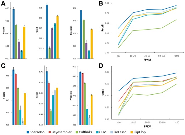
Performance evaluation on whole transcriptome simulation data. (A) single-end data and (C) paired-end data. The relationship between recall and FPKM: (B) single-end data and (D) paired-end data

We further evaluated the performance of all assemblers under different simulated abundance. Figure 3B and D shows the curve representing the relationship between the recall and simulated abundance of single-end data and paired-end data, respectively. The abundance of isoforms is quantified in FPKM. As shown in the figure, SparseIso had higher recall under a different level of abundance consistently, especially for lowly expressed isoforms (FPKM < 10). Lowly expressed isoforms are of a limited number of sequenced reads, making them difficult to be identified from candidate isoforms. For the deterministic methods such as IsoLasso and CEM, isoforms of low abundance are likely to be filtered out as noise by the thresholding step. By the virtue of the sampling approach in SparseIso, we estimated the joint probability distribution of all the candidate transcripts. The lowly expressed isoforms would still have a high chance to be selected. In Bayesembler, it first samples the number of expressed isoforms based on a Bayesian inference framework. If the number of expressed isoforms is lower than the sampled value, some isoforms are randomly selected as expressed even though they are from the unexpressed group. Different from Bayesembler, SparseIso considers the correlation of structure of all isoforms instead of random selection. The reads are fitted to all candidate isoforms rather than those in the expressed group only, which allows the isoforms in the unexpressed group to carry some noisy reads. As guided by the isoform structure, SparseIso can help identify more truly expressed transcripts than Bayesembler. To further evaluate the methods with different aligners, we compared the performances using HISAT2 aligner v2.1.0 and STAR aligner v2.5.3 (Supplementary Figs S2-3 and S2-4). Bayesembler was not included in this study as the software package was only compatible with Tophat2 aligner. The results showed that SparseIso outperformed existing methods with different alignment tools.

3.2 Performance evaluation with different numbers of expressed transcripts

As we observed that the complexity of the splicing graph structure increased drastically with the number of expressed transcripts in the gene, we categorized the RefSeq genes into different groups based on the number of annotated isoforms of each gene. We selected genes with a number of isoforms of 1 to 8, which covered more than 98% of genes. For each group of genes, we randomly selected 80 to 150 genes to generate both single-end and paired-end simulation data using RNASeqReadSimulator (Li and Jiang, 2012). The abundances of isoforms (the number of reads per base) were simulated from a Gamma distribution with mean 0.5 and variance 2. To maintain the complexity of the graph, we confirmed that every simulated isoform was expressed in the data by setting a low threshold of 0.05 to the isoform expressions. The number of reads simulated was set proportional to the expression level of all the isoforms in a range of 10 to 20 million. The read length was set as 100 for both types of data. For the paired-end data, the fragment length was simulated from a Gaussian distribution with a mean of 200 and standard deviation of 20 (the default setting of RNASeqReadSimulator). We generated 10 simulation datasets for each case to evaluate the standard deviation of the performance.

Figure 4A, B and C show the F-score, recall and precision in the paired-end data study. The performance of single-end study is shown in Supplementary Figure S2-5. It can be seen from the figures that SparseIso outperformed all the existing methods regarding F-score, especially for the genes with a higher number of isoforms. Among the existing methods, Bayesembler performed the best, demonstrating the advantage of using the sampling strategy. As the structure of single-isoform genes is very simple, all method can achieve an F-score over 0.95. In all the eight groups of genes, the precisions of all methods were comparable, while SparseIso achieved a significantly improved performance in terms of recall. When the number of isoforms is low, the number of candidate isoforms enumerated from the splicing graph is small. All assemblers can achieve great performance in inferring true isoform structures from a small set of candidate isoforms. As the number of isoforms in genes increases, the complexity of the splicing graph increases drastically. To maintain the precision, all the methods need to remove the potential false positive calls, which decreases the recall performance. It can be seen that Cufflinks achieved most accurate results for the genes with the number of isoforms of 6 to 8, but the recall was very low. Moreover, we further tested the precision performance when all methods had similar performance of recall. We set different thresholds of the predicted isoform abundance for all the methods to make them have the same recall performance (as the lowest recall value among all assemblers). Figure 4D shows the precision of the four methods with the same recall performance. It can be seen that SparseIso achieved higher precision than other competing methods.

Fig. 4.

Performance evaluation on paired-end simulation data. (A) overall performance of isoform identification evaluated by F-score; (B) recall performance; (C) precision performance; (D) precision performance when all as assemblers operate at the same recall performance

3.3 Performance evaluation by real RNA-seq data

We applied SparseIso and existing methods onto three human MCF7 breast cancer cell line data and three H1 embryonic stem cell line data [acquired in the ENCODE project (Djebali et al et al., 2012)] to identify isoforms. The raw sequences were downloaded from the UCSC genome browser (Rosenbloom et al., 2015), which consist of about 50 to 70 million reads of 76 bps paired-end data sequenced on Illumina platform in each sample. The detail information of the cell line data used in this study is summarized in Supplementary Table S2-1. All the reads were aligned to the UCSC human genome hg19 by Tophat2 (v2.0.11).

We first evaluated the performance of assemblers by comparing the identified isoforms with a reference isoform set. As the ground-truth of expressed isoforms is not available for the ENCODE data, we opted to use an alternative to evaluate the performance of competing methods in terms of precision and recall. Recently, several studies used Pacific Biosciences (PacBio) sequencing platform to identify novel transcript isoforms. Different from high-throughput RNA-seq technology, the PacBio sequencing platform can generate much longer reads with a relatively lower throughput than the Illumina platform. As the read length is much longer, the reads can span multiple splicing junctions or entire transcript, which alleviates the problem of inferring the combination of splicing junctions. In this study, we used the MCF7 transcriptome assembled by PacBio (http://www.pacb.com/blog/data-release-human-mcf-7-transcriptome/) and the H1 transcriptome assembled by a hybrid method of Illumina and PacBio reads (Au et al., 2013) to validate our identified isoforms from short sequenced RNA-seq reads. Consider the sensitivity of PacBio sequencing platform, some lowly expressed isoforms might not be sequenced. To comprehensively evaluate the performance, we combined the PacBio assembled transcriptome with known, annotated transcripts from RefSeq genes as a reference isoform set to compare with the identified isoforms.

Considering the estimated abundance bias of identified isoforms among assemblers, we used a curve-based method to evaluate the performance (Maretty et al., 2014). By adjusting the threshold of abundance from high to low, we can generate different numbers of identified transcripts for each method, and calculate the number of matched transcripts. Then we can plot a curve of the number of matched transcripts against the corresponding number of predicted transcripts. The slope and height of the curve represent the precision and recall of the assemblers. Figure 5A and Supplementary Figure S2-6 show the curves for MCF7 replicates, and the curves for H1 replicates are shown in Figure 5B and Supplementary Figure S2-7. The curves are very similar for the replicates of the same cell line. It can be seen from the figure that the curves of SparseIso and Bayesembler increase much faster and finally reach a higher point than the other assemblers, showing that the two methods are of a significant performance advantage in terms of precision and recall. Compared with Bayesembler, SparseIso exhibits a similar performance in precision and recall for detecting top 15 000 isoforms. However, the curve of SparseIso increases much faster and higher later on, which shows that SparseIso has a significant improvement over Bayesembler in both precision and recall for identification of the isoforms of relatively low abundance. Besides the performance evaluation at the transcript level, we also showed the improved performance of SparseIso at the gene level (Supplementary Section S1.9).

Fig. 5.

Performance evaluation of all assemblers on MCF7 and H1 cell line data using PacBio transcriptome and RefSeq annotation: (A) MCF7-rep1 and (B) H1-rep1

Finally, we examined the consistency of assembled transcripts from multiple replicates to evaluate the performance. The use of multiple runs of MCF7 and H1 cell line data in our study provided a pairwise validation between data to validate the identified isoforms. Even if an isoform cannot be verified in known annotation, we would confirm the expression of the isoform if the same splicing structure is observed in another sample. We defined the confirmed set of isoforms as the identified isoforms from two datasets sharing the same intron chain. We employed a pairwise comparison between the identified isoform sets from the three replicates of the same cell type. We also set different thresholds on abundance to generate isoform sets with different sizes and plotted the curve of the number of confirmed transcripts against the corresponding number of predicted transcripts. The pairwise comparison curves for all the cell line data are shown in Figure 6, Supplementary Figures S2-8 and S2-9. It can be seen that the identified isoforms from SparseIso are much more consistent across different runs than other assemblers. The performance of SparseIso is the highest among all assemblers in terms of precision and recall. Compared with the isoforms validated by the reference isoform set, SparseIso identified more than 1011 (7.45%) verified isoforms in average.

Fig. 6.

Pairwise comparison of identified isoforms by all assemblers: (A) MCF7-rep1 vs. MCF7-rep2 and (B) H1-rep1 vs. H1-rep2

3.4 Breast cancer cell line study

To further demonstrate the effectiveness of SparseIso in real data study, we evaluated the isoforms identified from the MCF7 cell line [ENCODE project (Djebali et al., 2012)] on another MCF7 time-course RNA-seq data (GEO accession no. GSE62789) (Honkela et al., 2015). The MCF7 data were sequenced at 10 time points: 0, 5, 10, 20, 40, 80, 160, 320, 640 and 1280 min after E2 stimulation. We downloaded the raw sequence data and aligned to the hg19 reference genome by TopHat2. To build a reference isoform set for quantification, we first categorized the identified isoforms by comparing with the RefSeq annotation using the tool Cuffcompare. Cuffcompare uses 12 class codes to annotate the identified isoforms. Among all identified isoforms, we selected the potentially novel isoforms (class code ‘j’) identified in more than one replicates as a complement to the RefSeq annotation. In total, the reference isoform set consists of 11 023 novel isoforms and 57 240 known isoforms from RefSeq annotation. We estimated the abundance of reference isoform set using RSEM (Ratkiewicz et al., 2011). If one isoform has FPKM of less than 1 in one sample, it is labeled as not expressed in the sample. We filtered out all the isoforms that do not express in more than 8 samples. The expression of isoforms was further transformed to log scale from FPKM. We further filtered out all the isoform with variance less than 2 for analysis. Finally, we applied hierarchical clustering on the isoforms originated from the genes (2113 genes and 5955 isoforms) having at least one novel isoform identified. The isoforms formed four clusters with different patterns. The heatmap is shown in Supplementary Figure S2-12. The corresponding genes in each cluster were analyzed using DAVID functional analysis tool (Huang et al., 2008). The details of the functional annotation results can be found in Supplementary Table S2-2. The functional analysis results show that all clusters are enriched in cell cycle and DNA repair, which are closely related to cell development. Cluster 1 and 4 are more enriched in breast cancer related signaling pathways (Table 1) such as ErbB signaling pathway, FoxO signaling pathway, AMPK signaling pathway and NFKB signaling pathway. Especially, AMPK signaling pathway is shown to be related to E2 stimulation (Lipovka et al., 2015). In addition, we have also found 702 genes that have alternative isoforms with different expression patterns, which indicates that the isoforms of the same gene may have different functional roles in biological systems. Some of the genes have been demonstrated to have alternative isoforms with different activities. For example, NUMB has six isoforms with distinct functions in cancer (Karaczyn et al., 2010) and the isoforms of DVL express substantially different in different breast cancer cell lines (Schlange et al., 2007).

Table 1.

Breast cancer related pathways enriched in Cluster 1 and 4

Cluster	Enriched pathways and GO functions	P-value
Cluster 1	FoxO signaling pathways	5.9E-3
	ErbB signaling pathways	8.5E-3
	AMPK signaling pathways	1.2E-2
Cluster 4	NFKB signaling pathway	9.9E-2
	ErbB signaling pathway	9.9E-2

4 Discussion

We develop a new Bayesian approach to identify expressed isoforms from RNA-seq data. Comparing with existing read count-based methods, we consider the reads falling on both splice junctions and exons. The inclusion of junction counts in the model helps resolve the read assignment better. Taking the advantage of paired-end RNA-seq data, we also incorporate the concept of paired-end modules to better estimate the abundance level. Considering the positional bias and sequencing bias in the RNA-seq experiment, we use an NB model together with a global bias curve introduced in (Wu et al., 2011) to address the count variation. The abundance levels of segments are modeled as a mixture of counts from isoforms. Sparsity in expressed isoforms is enforced by a spike-and-slab prior distribution. The model parameters are iteratively estimated by a Gibbs sampling procedure. Different from deterministic approaches, our sampling approach iteratively estimates the joint posterior distribution rather than thresholding the lowly expressed isoforms. It is not necessary that an expressed isoform must be highly expressed. Instead of using the abundance of isoforms as a measure, we calculate the confidence level as a statistical measure to prioritize all candidate transcripts.

Compared with Bayesembler (a sampling-based method as recently developed), our SparseIso has several improvements for isoform identification. Bayesembler identifies all transcripts with nonzero counts as expressed transcripts, which may include some transcripts mainly constructed by error reads. In contrast, Our SparseIso method allows the false transcripts to have reasonable low abundance. As described in (Maretty et al., 2014), Bayesembler determines the number of expressed transcripts before assigning the reads to the expressed transcripts. It will randomly sample transcript index from the unexpressed set of transcripts if the estimated number of expressed isoforms is greater than the number of isoforms with the nonzero count. Assigning reads to a subset of candidate transcripts provides a local view of isoform selection; some reads, however, may be incorrectly assigned to unexpressed isoforms. In SparseIso, we sample the transcript abundance considering all candidate isoforms to find a global view of isoform selection. The preference of selecting isoforms is determined by both the expression state and the correlation of isoform structure modeled in the covariance matrix.

Funding

This work is supported by National Institutes of Health (NIH) [CA149653, CA164384, CA149147, CA184902, CA148826 and CA187512].

Conflict of Interest: none declared.

References

- Au K.F. et al. (2013) Characterization of the human ESC transcriptome by hybrid sequencing. Proc. Natl. Acad. Sci. USA, 110, E4821–E4830. [DOI] [PMC free article] [PubMed] [Google Scholar]
- Bernard E. et al. (2014) Efficient RNA isoform identification and quantification from RNA-Seq data with network flows. Bioinformatics, btu317. [DOI] [PMC free article] [PubMed] [Google Scholar]
- Damien P., Walker S.G. (2001) Sampling truncated normal, beta, and gamma densities. J. Comput. Graph. Stat., 10, 206–215. [Google Scholar]
- Djebali S. et al. (2012) Landscape of transcription in human cells. Nature, 489, 101–108. [DOI] [PMC free article] [PubMed] [Google Scholar]
- Dobin A. et al. (2013) STAR: ultrafast universal RNA-seq aligner. Bioinformatics, 29, 15–21. [DOI] [PMC free article] [PubMed] [Google Scholar]
- Griebel T. et al. (2012) Modelling and simulating generic RNA-Seq experiments with the flux simulator. Nucleic Acids Res., 40, 10073–10083. [DOI] [PMC free article] [PubMed] [Google Scholar]
- Guttman M. et al. (2010) Ab initio reconstruction of cell type-specific transcriptomes in mouse reveals the conserved multi-exonic structure of lincRNAs. Nat. Biotechnol., 28, 503–510. [DOI] [PMC free article] [PubMed] [Google Scholar]
- Hansen K.D. et al. (2010) Biases in Illumina transcriptome sequencing caused by random hexamer priming. Nucleic Acids Res., 38, e131.. [DOI] [PMC free article] [PubMed] [Google Scholar]
- Honkela A. et al. (2015) Genome-wide modeling of transcription kinetics reveals patterns of RNA production delays. Proc. Natl. Acad. Sci. USA, 112, 13115–13120. [DOI] [PMC free article] [PubMed] [Google Scholar]
- Huang D.W. et al. (2008) Systematic and integrative analysis of large gene lists using DAVID bioinformatics resources. Nat. Protoc., 4, 44–57. [DOI] [PubMed] [Google Scholar]
- Ishwaran H., Rao J.S. (2005) Spike and slab variable selection: frequentist and Bayesian strategies. Ann. Stat., 33, 730–773. [Google Scholar]
- Jiang H., Wong W.H. (2009) Statistical inferences for isoform expression in RNA-Seq. Bioinformatics, 25, 1026–1032. [DOI] [PMC free article] [PubMed] [Google Scholar]
- Karaczyn A. et al. (2010) Two novel human NUMB isoforms provide a potential link between development and cancer. Neural Dev., 5, 31. [DOI] [PMC free article] [PubMed] [Google Scholar]
- Karolchik D. et al. (2014) The UCSC genome browser database: 2014 update. Nucleic Acids Res., 42, D764–D770. [DOI] [PMC free article] [PubMed] [Google Scholar]
- Kim D. et al. (2013) TopHat2: accurate alignment of transcriptomes in the presence of insertions, deletions and gene fusions. Genome Biol., 14, R36. [DOI] [PMC free article] [PubMed] [Google Scholar]
- Li B., Dewey C.N. (2011) RSEM: accurate transcript quantification from RNA-Seq data with or without a reference genome. BMC Bioinformatics, 12, 323.. [DOI] [PMC free article] [PubMed] [Google Scholar]
- Li W. et al. (2011) IsoLasso: a LASSO regression approach to RNA-Seq based transcriptome assembly. J. Comput. Biol. J. Comput. Mol. Cell Biol., 18, 1693–1707. [DOI] [PMC free article] [PubMed] [Google Scholar]
- Li W., Jiang T. (2012) Transcriptome assembly and isoform expression level estimation from biased RNA-Seq reads. Bioinformatics, 28, 2914–2921. [DOI] [PMC free article] [PubMed] [Google Scholar]
- Lipovka Y. et al. (2015) Oestrogen receptors interact with the α-catalytic subunit of AMP-activated protein kinase. Biosci. Rep., 35, e00264. [DOI] [PMC free article] [PubMed] [Google Scholar]
- Maretty L. et al. (2014) Bayesian transcriptome assembly. Genome Biol., 15, 501.. [DOI] [PMC free article] [PubMed] [Google Scholar]
- Mezlini A.M. et al. (2013) iReckon: simultaneous isoform discovery and abundance estimation from RNA-seq data. Genome Res., 23, 519–529. [DOI] [PMC free article] [PubMed] [Google Scholar]
- Mitchell T.J., Beauchamp J.J. (1988) Bayesian variable selection in linear regression. J. Am. Stat. Assoc., 83, 1023–1032. [Google Scholar]
- Mortazavi A. et al. (2008) Mapping and quantifying mammalian transcriptomes by RNA-Seq. Nat. Methods, 5, 621–628. [DOI] [PubMed] [Google Scholar]
- Piegorsch W.W. (1990) Maximum likelihood estimation for the negative binomial dispersion parameter. Biometrics, 46, 863–867. [PubMed] [Google Scholar]
- Pruitt K.D. et al. (2014) RefSeq: an update on mammalian reference sequences. Nucleic Acids Res., 42, D756–D763. [DOI] [PMC free article] [PubMed] [Google Scholar]
- Ratkiewicz J. et al. (2011) Detecting and tracking political abuse in social media. ICWSM, 11, 297–304. [Google Scholar]
- Roberts A. et al. (2011) Improving RNA-Seq expression estimates by correcting for fragment bias. Genome Biol., 12, R22. [DOI] [PMC free article] [PubMed] [Google Scholar]
- Rosenbloom K.R. et al. (2015) The UCSC genome browser database: 2015 update. Nucleic Acids Res., 43, D670–D681. [DOI] [PMC free article] [PubMed] [Google Scholar]
- Schlange T. et al. (2007) Autocrine WNT signaling contributes to breast cancer cell proliferation via the canonical WNT pathway and EGFR transactivation. Breast Cancer Res., 9, R63. [DOI] [PMC free article] [PubMed] [Google Scholar]
- Trapnell C. et al. (2010) Transcript assembly and quantification by RNA-Seq reveals unannotated transcripts and isoform switching during cell differentiation. Nat. Biotechnol., 28, 511–515. [DOI] [PMC free article] [PubMed] [Google Scholar]
- Wang E.T. et al. (2008) Alternative isoform regulation in human tissue transcriptomes. Nature, 456, 470–476. [DOI] [PMC free article] [PubMed] [Google Scholar]
- Wu Z. et al. (2011) Using non-uniform read distribution models to improve isoform expression inference in RNA-Seq. Bioinformatics, 27, 502–508. [DOI] [PubMed] [Google Scholar]
Associated Data
This section collects any data citations, data availability statements, or supplementary materials included in this article.