Orthologous Matrix (OMA) algorithm 2.0: more robust to asymmetric evolutionary rates and more scalable hierarchical orthologous group inference

Abstract

Motivation

Accurate orthology inference is a fundamental step in many phylogenetics and comparative analysis. Many methods have been proposed, including OMA (Orthologous MAtrix). Yet substantial challenges remain, in particular in coping with fragmented genes or genes evolving at different rates after duplication, and in scaling to large datasets. With more and more genomes available, it is necessary to improve the scalability and robustness of orthology inference methods.

Results

We present improvements in the OMA algorithm: (i) refining the pairwise orthology inference step to account for same-species paralogs evolving at different rates, and (ii) minimizing errors in the pairwise orthology verification step by testing the consistency of pairwise distance estimates, which can be problematic in the presence of fragmentary sequences. In addition we introduce a more scalable procedure for hierarchical orthologous group (HOG) clustering, which are several orders of magnitude faster on large datasets. Using the Quest for Orthologs consortium orthology benchmark service, we show that these changes translate into substantial improvement on multiple empirical datasets.

Availability and Implementation

This new OMA 2.0 algorithm is used in the OMA database (http://omabrowser.org) from the March 2017 release onwards, and can be run on custom genomes using OMA standalone version 2.0 and above (http://omabrowser.org/standalone).

1 Introduction

Inferring evolutionary relationships between genes lies at the heart of comparative, phylogenetic, and functional analyses. Homologs are genes that share a common ancestry (Fitch, 1970). They can be further classified into: orthologs if they arose by speciation events, or paralogs if they arose by duplication events (Fitch, 1970; Fig. 1). These evolutionary relations are all defined among pairs of genes and—except for homology—are not transitive. Many orthology inference methods have been proposed over the years, such as COGs (Tatusov et al., 1997), bidirectional best hits (Overbeek et al., 1999), Inparanoid (Remm et al., 2001), OrthoMCL (Li et al., 2003), Ensembl Compara (Vilella et al., 2008) or OrthoDB (Kriventseva et al., 2008).

Fig. 1.

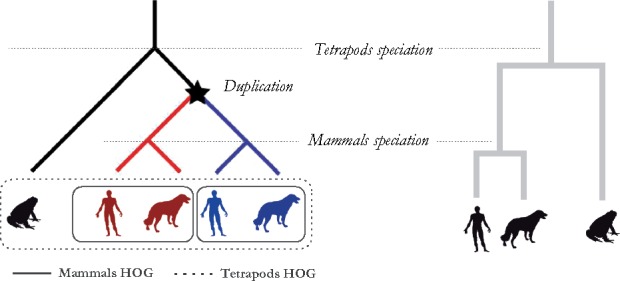
Hierarchical Orthologous Groups. Labeled gene tree (left) and its related species tree (right) illustrating the evolutionary history of five genes all descended from a single common ancestral at the tetrapods level. Those homologs can be classified as orthologs if they start diverging by speciation (human versus dog genes of same color) or as paralogs if they start diverging by duplication (blue versus red genes). We can identify in this example HOGs at two taxonomic levels: one larger HOG at the tetrapods level (dotted-line rectangle) containing all the homologous genes that emerged from the single tetrapod ancestral gene, and two HOGs at the mammalian level (solid-line rectangles), due to a duplication of the tetrapod ancestral gene before the mammals speciation

The Orthologous Matrix (OMA) algorithm infers orthologous genes among multiple genomes on the basis of protein sequences (Dessimoz et al., 2005; Roth et al., 2008). In addition to inferring such pairwise evolutionary relationships, OMA infers two types of orthologous groups. The first, called ‘OMA groups’, are sets of genes in which every pair is inferred to be orthologous. The second, introduced more recently and called ‘hierarchical orthologous groups’ (HOGs), are defined as set of genes that have all descended from a single common ancestral gene at a specific taxonomic range of interest (Altenhoff et al., 2013; Fig. 1).

When compared with most other methods, the OMA algorithm has been shown to have high precision (i.e. low false-positive rate) but low recall (i.e. high false-negative rate) in several benchmark studies (Altenhoff and Dessimoz, 2009; Altenhoff et al., 2016; Boeckmann et al., 2011; Trachana et al., 2011). Even so, predicting correct evolutionary relationships becomes more difficult due to complex mechanisms such as differential gene loss, asymmetric evolutionary rates, gene duplications and poor quality genomes. This can lead to spurious or missing relationships (Dalquen and Dessimoz, 2013).

The final stage of the OMA pipeline infers HOGs from pairwise orthologs (Altenhoff et al., 2013). Such groups are useful for analyzing multiple genomes or genes, but require scalable clustering algorithms due to the complexity in reconstructing them.

Here, we present two new improvements to our orthology inference algorithm in order to better handle rapidly evolving duplicated genes and to improve detection of asymmetric gene loss. In addition, we introduce a ‘bottom-up’ HOGs clustering algorithm that can scale up to thousands of genomes.

2 Materials and methods

We first provide an overview of the OMA algorithm, then present in details the three refinements introduced in this new version, and finally provide methodological details about the benchmarking.

2.1 Overview the OMA algorithm

The following section provides an overview of the existing OMA algorithm, of which the details are described in (Roth et al., 2008).

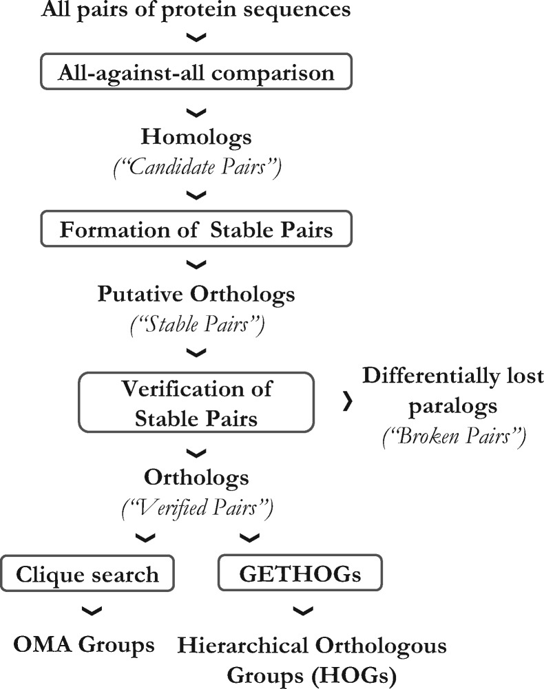
The OMA algorithm infers pairs of orthologous genes from complete genomes in a four-step process (Fig. 2):

Fig. 2.

Overview of the OMA pipeline. Boxes denote individual steps in the pipeline, while the text outside boxes denotes the input or output of these processes and their terminology in OMA

1. Homology inference: Alignments are made with all possible pairs of sequences from all genomes using local dynamic programming (Smith and Waterman, 1981), and pairs with sufficient score and overlap are promoted to Candidates Pairs.

2. Ortholog and co-ortholog inference: Candidates Pairs that are the mutually evolutionary closest sequences between a pair of genomes are upgraded to Stable Pairs. In order to include many-to-many orthologous relationships, Candidate Pairs found within a confidence interval (corresponding to distance variance) are also upgraded to Stable Pairs.

3. Witness of non-orthology verification: At this point, some pairs of paralogs may still be misidentified as orthologs due to differential gene loss (Dessimozet al.,2006a). To avoid such cases, a verification step is added to assess the orthologous origin of a Stable Pair by using a third genome that retained both orthologous copies, which thus act as witnesses of non-orthology. Pairs that pass this test are upgraded to Verified Pairs.

4. Ortholog clustering: Once the pairwise orthologs are inferred, a clustering algorithm is applied to group genes descending from a common ancestral gene into HOGs.

2.2 Algorithmic refinements: taking into account fast-evolving duplicated genes in the orthology inference step

In the current orthology inference step of the OMA algorithm, genes that are mutually the closest pairs of sequences across genomes are considered as putative orthologs. Due to lineage-specific duplications, orthology relationships are however not necessarily one-to-one (e.g. Dalquen and Dessimoz, 2013). Thus, OMA considers a tolerance interval during the mutually closest gene search to allow for inclusion of potential inparalogs.

Specifically, the criterion originally used in OMA was as follows: a Candidate Pair xy between genomes X and Y is upgraded to a Stable Pair if for all genes x_i from X and for all genes y_j from Y with x_i ≠ x and y_j ≠ y:

$$d_{x{y}_{\mathrm{j}}}-d_{xy}>-k * \text{stdev}\left(d_{x{y}_j}-d_{xy}\right)$$

             and

$$d_{x_{i}y}-d_{xy}>-k * \text{stdev}\left(d_{x_{i}y}-d_{xy}\right)$$

where d is the pairwise maximum likelihood distance estimate, k the tolerance parameter of the standard deviation between the two distances, and where stdev() is the distance standard deviation of the difference (Dessimoz et al., 2006a,b). This means that a Candidate Pair xy is upgraded to a Stable Pair if and only if there are no other pairs xy_j or yx_i with significantly smaller evolutionary distances.

So far in the orthology inference step, only the distances between genes from different genomes are taken into account. However, if a duplicated gene evolved faster than its related in-paralog, searching for mutually closest genes between genomes can fail to identify it as an ortholog (Fig. 3A). Because of the distance asymmetry, the original algorithm does not detect the fast evolving gene as a co-ortholog, thus wrongly implying an ancestral duplication as the origin of divergence (Fig. 3B).

Fig. 3.

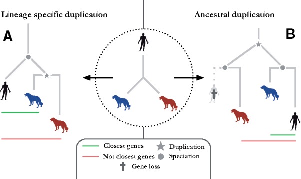
Putative evolutionary scenario for a gene triplet containing 1 human gene and 2 asymmetrically evolving dog genes. (A) Reconciled labeled gene tree for the gene triplet where the red dog gene (orthologous to the human gene) evolved at faster rate of evolution. (B) Reconciled labeled gene tree for the gene triplet where an ancestral duplication gave rise on one side to the blue dog gene and the black human gene and on the other side only to the red dog gene, since the related gray human gene had been lost. The red dog gene is thus paralogous to the black human gene

The refinement introduced here also takes into account the evolutionary distance between inparalogs. Inspired by other orthology algorithms detecting co-orthologs on the basis of alignment scores, such as Inparanoid (Remm et al., 2001) or OrthoInspector (Linard et al., 2011), we added a new check that the distance between the two potential in-paralogous dog genes is significantly smaller than the distance between the closest genes (black and blue genes), as illustrated in the Figure 3A. More precisely, we retain as Stable Pairs all Candidate Pairs xy between genomes X and Y that were previously discarded during orthology inference if, for any genes y_j from Y with y_j ≠ y there exists a gene y_i that has a distance to y significantly closer than the distance between the Candidate Pair genes x and y₂:

$$d_{xy}-d_{y{y}_j}>-k * stdev\left(d_{xy}-d_{y{y}_j}\right)$$

where d is a pairwise maximum likelihood distance estimate, k the inparalogs tolerance parameter of the standard deviation between the two distances and where the distance standard deviation stdev() is computed according to Dessimoz et al. (2006a,b).

2.3 Algorithmic refinements: extended witnesses of non-orthology with verification of distances additivity

As mentioned earlier, the verification step of the OMA algorithm aims at detecting paralogs resulting from differential gene losses (Fig. 4A). Indeed, paralogs can be the only remaining homologs between two genomes and since they are mutually the closest genes across those genomes they can be wrongly inferred as orthologs. To prevent such cases, OMA searches for each pair of putative orthologs (‘Stable Pairs’) whether there might be a third genome that has retained paralogs that could act as a witness of non-orthology (Dessimoz et al., 2006a,b).

Fig. 4.

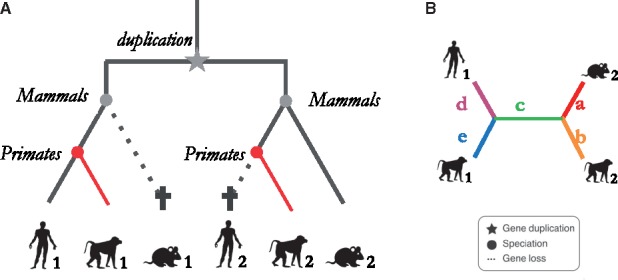
Hidden paralogs example and witness of non-orthology gene quartet. (A) Example of labeled gene tree containing hidden paralogs due to asymmetric gene losses between human and mouse. This can occur when an ancestral duplication is first followed by a speciation then by asymmetric genes losses. The resulting paralogs are wrongly inferred as orthologs because they are the mutually closest pairs between two genomes (Human₁, Mouse₂ sequences). OMA attempts to identify such cases through the use of a third species (here a monkey) that has retained both copies, which can act as witnesses of non-orthology.(B) The four extant genes form a quartet with branches labeled a–e

This test is based on pairwise evolutionary distance comparison of the gene quartet, without reconstructing the underlying gene tree (which, given the very large number of quartets of homologous genes across many genomes, would be too time consuming). However, direct comparison of pairwise distances implies that the distances among the four genes are additive, and by consequence, that a phylogenetic tree can be reconstructed from them. We have found cases, particularly in the presence of fragmentary sequences, where additivity is far from being met.

To ensure that the evolutionary distances do not depart excessively from additivity, in the verification of Stable Pair x₁,y₂ using potential witnesses of non-orthology z₁,z₂, we test a ‘soft’ variant of the four-point condition (Buneman, 1974), which allows for distance estimation uncertainty. We check that the sum of the distances d(x₁,z₂) and d(y₂, z₁) is approximately equal to the sum of the distances d(x₁, y₂) and d(z₁, z₂). Indeed, considering the branch labels defined in Figure 4B, under the model and assuming no error, the following equality holds:

$$\left(d+c+b\right)+\left(a+c+e\right)=\left(d+c+a\right)+\left(e+c+b\right)$$

Taking inference uncertainty into account, we test the equality as follows:

$$\begin{array}{c}\hspace{0.17em}\hspace{0.17em}\hspace{0.17em}\hspace{0.17em}\hspace{0.17em}\hspace{0.17em}\hspace{0.17em}\hspace{0.17em}\hspace{0.17em}\hspace{0.17em}\hspace{0.17em}\hspace{0.17em}\hspace{0.17em}\hspace{0.17em}\hspace{0.17em}\hspace{0.17em}\hspace{0.17em}\hspace{0.17em}\hspace{0.17em}\hspace{0.17em}\hspace{0.17em}\hspace{0.17em}\hspace{0.17em}\hspace{0.17em}\hspace{0.17em}\hspace{0.17em}\hspace{0.17em}\hspace{0.17em}\hspace{0.17em}\left| d_{x_1{z}_2}+d_{y_2{z}_1}-d_{x_1{y}_2}-d_{z_1{z}_2} \right|<\\ 2* \sqrt{\text{var}\left( d_{x_1{z}_2}\right)+\text{var}\left(d_{y_2{z}_1}\right)+\text{var}\left(d_{x_1{y}_2}\right)+\text{var}\left(d_{z_1{z}_2}\right)}\end{array}$$

where x₁ and y₂ are the Stable Pair genes from genomes X and Y, z₁ and z₂ are the witnesses of non-orthology in the third genome Z, d is a pairwise maximum likelihood distance estimate, and var(d(x,y)) is the variance of the distance estimate between sequences x and y. If the test fails, z₁ and z₂ are not used as witnesses of non-orthology.

2.4 Algorithmic refinements: bottom-up HOG inference

In this section, we present improvements to the hierarchical orthologous group (HOG) clustering phase (Altenhoff et al., 2013). The work established a one-to-one correspondence between the connected components of a perfect orthology graph—i.e. containing no false positive or negative— and HOGs. Based on this, but allowing for a noisy input, we introduced a heuristic called GETHOGs (‘Graph-based Efficient Technique for Hierarchical Orthologous Groups’), which used the min-cut algorithm to break down spurious orthologous relationships before identifying HOGs as the connected components. This was performed for each taxonomic range of a reference phylogeny, starting from the root and walking down the tree to the most specific clades, in a ‘top-down’ fashion.

Nevertheless, inconsistencies in the orthology graph due to spurious inferences or missing relations increase the probability of making errors during the clustering. Such mistakes in grouping are then propagated during the entire clustering procedure due to the greedy nature of the algorithm, and can affect the final result. Furthermore, the original GETHOGs algorithm started at the root of the reference phylogeny, where the graph is largest (since it contains pairs of orthologs between all species instead of subsets of them) and most uncertain (since it also contains orthologous relationships among the most distant species).

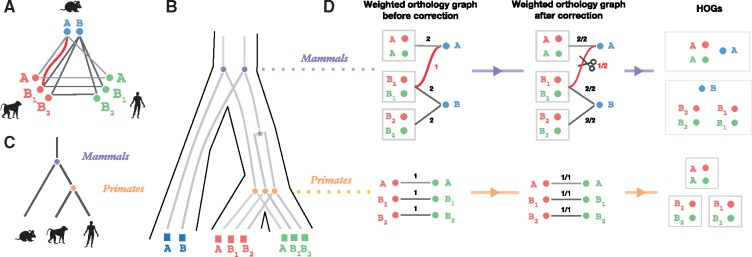
Here, we introduce a ‘bottom-up’ variant of GETHOGs, which infers HOGs starting with the most specific taxonomy and incrementally merges them toward the root (Fig. 6). More specifically, the new approach reconstructs HOGs by applying the following procedure with each speciation node of the species tree as reference, from the leaves to the root:

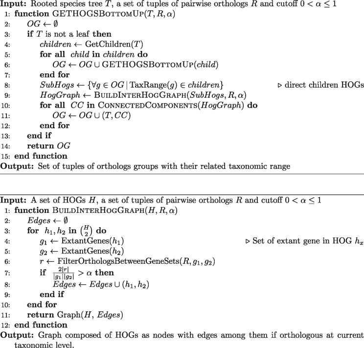
1. Build inter-HOG orthology graph (Fig. 5 BuildInterGraph, Fig. 6Dleft): Define a graph in which the nodes are the HOGs inferred at the level of each child of the reference speciation. If a child is a leaf of the species tree (i.e. a child is an extant species), the HOGs defined at this level are simply the individual sequences of that species. The edges of the graph represent one or more pairwise orthology relationships between members of the HOGs, with the number of such relationships recorded as weights.

2. Remove spurious edges (Fig. 5 BuildInterGraph line 7–9, Fig. 6Dmiddle): Once the orthology graph is built, we next assess whether each edge is well supported or not. For each edge, the algorithm computes the ratio of the number of pairwise orthologous relations (edge weight) to the maximum number of possible pairwise orthologous relations (equal to the product of the size of the two HOGs connected by the edge). If the input orthology graph is perfect (i.e. correct and complete), this ratio is one. A cutoff α (set to 0.8 throughout this article and by default) is then used to remove all edges with insufficient connections.

3. Search for connected components (Fig. 5 GETHOGSBottomUp line 10–12, Fig. 6Dright)): The final step searches for connected components inside the graph and clusters them together as a single HOG at the level of the speciation of reference.

The asymptotic complexity is determined by the complexity of the species tree traversal and the complexity for the HOG inference at each internal node of the species tree (i.e. inference for each taxonomic level). Tree traversal has a runtime complexity of O(n) where n is the number of species, because there are n-1 internal nodes. The runtime of the HOG inference at each level (steps 1–3 above) primarily depends on the number of pairwise orthology relationships. The total number of sequences is O(n) because we can expect a natural limit on the size of each genome. Thus, the total number of pairwise relationships is O(n²). Using Union-Find data structures, finding connected components in a graph of m edges is O(m) (Cormen, 2009). There are potentially O(n²) edges in each inter-HOG orthology graph, but since each orthology relationship only need to be considered once in the entire traversal (at the speciation node which induces them), the amortized complexity at each internal node is O(n) resulting in a total complexity of bottom-up GETHOGs of O(n²). This compares favorably to the top-down GETHOG algorithm, which has complexity O(n³·log⁴n) (Altenhoff et al., 2013).

Fig. 6.

Bottom-up GETHOGs reconstruction example. (A) Orthology graph, where circles represent extant genes with a species-specific color and edges represent pairwise orthologous relations between genes. The red edge represents a spurious orthologous relation between the mouse gene A and the monkey gene B₁. (B) Reconciled gene trees corresponding to the orthology graph in (A). Extant genes are represented by squares, speciation events by circles and duplication events by stars. (C) Corresponding species tree. (D) HOGs reconstruction using bottom-up GETHOGs with a minimal edges removal threshold of 0.8. The algorithm starts by reconstructing HOGs at the level of the primates and finishes at the level of mammals. The left panel displays the sub-orthology graph composed of HOGs (or extant genes) as nodes connected by weighted edges according to the number of existing orthologous relations between HOG genes. In the middle panel, to identify spurious edges, GETHOGs computes the fraction of orthologous pairs over the maximal number of possible pairs. The algorithm removes the red edge because the score is smaller than the minimal edge removal threshold. The right panel depicts the HOGs reconstructed from the connected component of the corrected graph

Fig. 5.

Pseudocode of bottom-up GETHOGs algorithm

2.5 Validation and benchmarking

We used the Quest for Orthologs (QfO) reference proteomes dataset (Altenhoff et al., 2016) to benchmark our method and to analyze case studies. It consists of 66 (40 eukaryotes, 20 bacteria, 6 archaea) proteomes, and contains more than 750 000 non-redundant protein sequences. It includes a broad selection of genomes covering the tree of life, including model organisms of interest and those important in biomedical or phylogeny research. In addition, as a reference tree we used a manually curated species tree for the 66 organisms contained in the QfO reference proteomes (Boeckmann et al., 2015).

The orthology benchmarking service (http://orthology.benchmarkservice.org) is an automated web-based tool for orthology inferences quality assessment (Altenhoff et al., 2016). This service takes ortholog relations inferred on the QfO reference dataset as input, and after running a broad range of tests, it summarizes and plots the results. We focused on the generalized species tree discordance test for our benchmark analysis, as it is a robust way to assess the quality of orthology predictions.

The generalized species tree discordance test estimates the agreement between orthology predictions and a reference species tree. Since orthologs originate by speciation, comparing the similarity of a tree reconstructed using pairwise orthology relations to a reference species tree is a way to assess the quality of the orthology predictions. We applied this procedure to a subset of the QfO references proteomes, covering different taxonomic ranges (Last Universal Common Ancestor, Eukaryotes, Vertebrates and Fungi). The main results provided by this test are the ‘error rate’ (average Robinson-Foulds distance between the reconstructed gene tree and reference species tree), the ‘number of complete trees sampled’ (number of trees fully reconstructed out of 50 k trials), and the ‘number of predicted orthologs’.

3 Results

Before presenting aggregate benchmarking results, we first present detailed examples of improvements obtained by the refinements described in the previous section. We begin with a case study of a family containing fast-evolving genes, where we recover orthologous relations and correct the orthology graph. We then present an example of the kind of improvement obtained by the new additivity test.

3.1 Fast-evolving duplicated genes case study: the haptoglobin family

The first orthology inferences refinement we present aims to include fast evolving duplicated genes in orthology predictions by not only looking at evolutionary distances between genomes but also within genomes.

In order to investigate the performance of this refinement, we used the haptoglobin gene family as an example, which duplicated in the primates (Fig. 7A). One branch of the primate paralogs evolved at a higher evolution rate than its sister branch, leading to asymmetry in the distance between the paralogs. As a result, although there is a one-to-many relationship between rodent haptoglobin and primate haptoglobin, the original OMA algorithm only uncovers the most conserved orthology pairs (Fig. 7B). By taking into account the relatively short distance between the in-paralogous copies (see section 2), the updated OMA algorithm now recovers both copies as co-orthologs to their rodent counterparts (Fig. 7C).

Fig. 7.

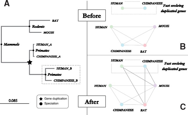
Analysis of haptoglobin gene family in mammals. (A) Phylogenetic labeled gene tree of the haptoglobin family built using 6 proteins sequences from 4 mammals (rat, mouse, human, chimpanzee). The dotted rectangle highlights the fast evolving primate paralogous genes. (B,C) Orthology graph of the haptoglobin gene family shown in A. Nodes represent extant genes denoted by a species-specific color and their identifier meanwhile the edges represent pairwise orthologous relations between genes. The orthology graph in B, relies on the pairwise orthologous relations inferred using the classic OMA algorithm, while the orthology graph in C is built using the orthology relations including the refinement for paralogs evolving at different rates. (UniProt IDs of the sequences involved Mouse→Q16646, Rat→A0A0H2UHM3, Human_a→HOY300, Chimpanzee_a→H2RAT6, Human_b→P00739, Chimpanzee_b→H2RB63)

3.2 Additivity of distances in witnesses of non-orthology step

As previously discussed in the section 2, the OMA algorithm attempts to uncover hidden paralogs (pairs of paralogs resulting from differential gene losses, thus each lacking an ortholog in the other species). This step compares evolutionary distances among quartets of genes without explicitly reconstructing their underlying phylogenetic gene tree (for performance reasons), under the assumption of near additivity of these distances.

However, in some cases—typically in the presence of one or more fragmented sequences—the assumption of additivity is strongly violated. Figure 8 shows an example of a quartet of genes with non-additive distances, where a Stable Pair between two mammal genes is erroneously discarded using two Arabidopsis genes as witnesses of non-orthology. The underlying phylogenetic gene tree (Fig. 8A) indicates that the Arabidopsis genes are in fact the result of a duplication within plants and not an ancestral duplication shared with the mammals in question. Without resorting to tree inference on a multiple sequence alignment (which would be prohibitively costly considering the number of quartets needed to verify every putative ortholog), the non-additivity of the pairwise distances in this quartet (Fig. 8B) can be detected by applying the new condition (see section 2), which in this case is violated:

Fig. 8.

Example of non additivity among gene quartet distances. (A). The two Arabidopsis genes arose from a duplication within the plants, which can be inferred from a tree inferred using a multiple sequence alignment. (B) However, if we consider pairwise distances estimated from independent pairwise alignments, one Arabidopsis gene appears to be closer to the human sequence, while the other appears to be closer to the opossum gene. In the original OMA algorithm, this would result in these Arabidopsis genes being erroneously used as witnesses of non-orthology; in the new algorithm, the non additivity of these distances (in Point Accepted Mutation units, with estimator variance in parentheses) is detected and the Arabidospsis genes are not used. (UniProt IDs of sequence involved: Human → Q16874, Opossum → F7FI80, Arabidopsis a → Q93ZB2, Arabidopsis b → Q9LNJ4)

The equation does not hold, thus we cannot rely on this pair of Arabidopsis genes as witnesses of non-orthology.

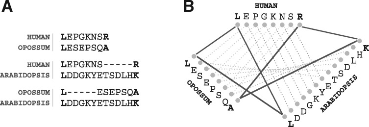
To understand how such non-additivity arises, consider that the evolutionary distances are computed independently during the all-against-all phase. As a result, the pairs of residues aligned (thus inferred to be homologous) can be inconsistent across the different sequences some inconsistencies and can appear within the pairwise alignments (non-conservation of homologous sites Fig. 9). In our example, the additivity test will fail; thus the Arabidopsis genes will not be used as witnesses of non-orthology, and the orthology inferred between the human and opossum sequence will stand (unless of course a different pair of witnesses, with additive distances this time, is found).

Fig. 9.

Example of non conservation of homologous sites across independent pairwise alignments. (A) Excerpts of three pairwise alignments between three sequences. (B) Graph-representation of the three alignments, where lines connect aligned residues. The lines are depicted as full lines if the characters are aligned consistently—thus forming closed triangles—and as dotted lines if they are aligned inconsistently—thus forming open triangles. (Sequence mapping to Uniprot Id: Human → H. sapiens|Q16874, Opossum → M. domestica|F7FI80, Arabidopsis → A. thaliana|Q93ZB2.)

3.3 QfO benchmarking results

To quantitatively assess the impact of the changes in the OMA algorithm, we submitted results obtained with them—individually and in combination—to the QfO orthology benchmark service (Altenhoff et al., 2016).

We first consider the results at the level of pairwise orthology (‘OMA Pairs’). Applying the new handling of asymmetrically evolving paralogs and the additivity test separately, we observe a significant increase in the number of predicted orthologs while maintaining a similar or even slightly better precision (Fig. 10). Precision here is measured in terms of average topological distance between the reference species tree and the gene tree reconstructed from the inferred orthologs (the lower the better). When the two refinements are combined, there is an even higher increase in the number of predicted orthologs compared with the current OMA predictions, while maintaining further the quality of the inferences. Consistent results are obtained for the different resolutions provided by the QfO benchmark service, though the increase in the number of inferred pairs is more modest in the fungal dataset (http://orthology.benchmarkservice.org/cgi-bin/gateway.pl?f=CheckResults&p1=25fe02429dc60c51f81da2de).

Fig. 10.

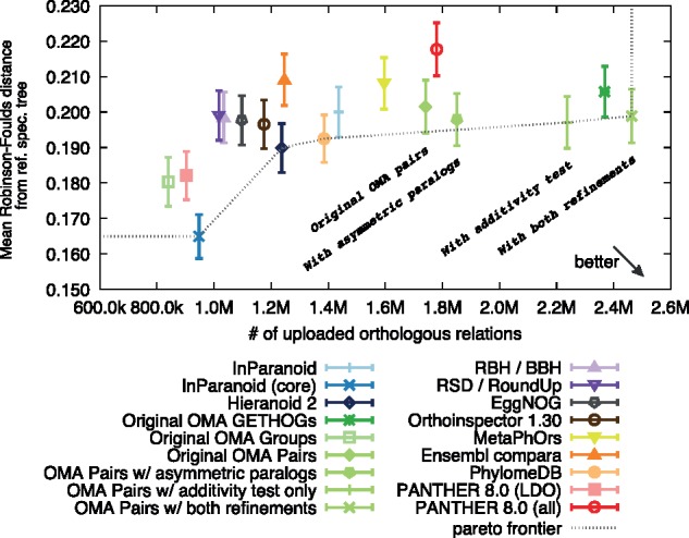
Effect of the refinements on pairwise orthology relationships (OMA Pairs) in the generalized species tree discordance test at vertebrate level. The asymmetric paralogs denotes the change in the OMA algorithm aiming to include fast evolving duplicated genes during orthology inferences. The additivity test denotes the new quartet consistency test added to the witness of non-orthology step. Error bars denote the 95% CI of the mean

Next, we turn to the improvements in HOG inference. As described in more detail in the section 2, the new HOG inference approach (‘bottom-up GETHOGs’) implements several modifications compared with the original version (Altenhoff et al., 2013): (i) The taxonomy is no longer traversed top-down but from the bottom-up, in a postfix traversal of the species tree; (ii) In the inter-HOG orthology graph considered for each clade, the nodes now represent HOGs instead of single genes, thereby considerably reducing the complexity of these graphs; (iii) The edges are weighted according to the number of orthology relations between two clusters of genes; (iv) Instead of cutting down spurious edges in the orthologous graph using a minimum cut algorithm, the bottom-up HOG inference enables us to assess the support of orthologous relationships between HOGs in terms of the total number of orthologous relationships that would be expected given perfect input pairwise orthologs.

To assess the impact of the change, we first compared the top-down and bottom-up variants on the QfO ortholog benchmark service on the original OMA pairs as input (i.e. without new asymmetric paralogy and additivity tests). The bottom-up algorithm resulted in a substantial increase in the numbers of predicted orthologs with the latter, indicating higher recall (Fig. 11). On the Eukaryotic, Vertebrate, and Fungal datasets, the error rate is also markedly lower, while on the universal dataset (including bacteria, archaea and eukaryotes), the error rate is about the same (http://orthology.benchmarkservice.org/cgi-bin/gateway.pl?f=CheckResults&p1=98f077d9d00d3ab0375be957).

Fig. 11.

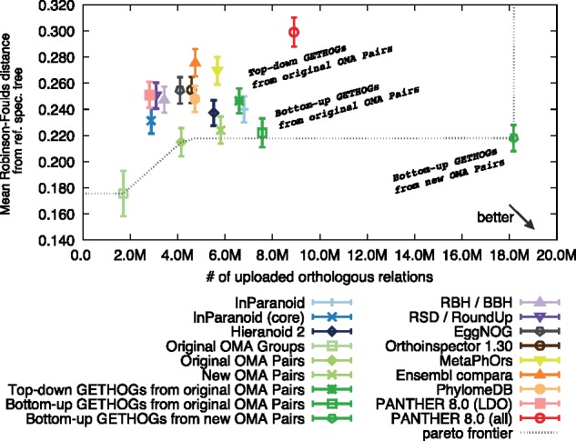
Assessment of HOG inference on the generalized species tree discordance test (eukaryotic dataset). Error bars denote the 95% CI of the mean. The data points with ‘original OMA’ refer to the algorithm used before this study and ‘new OMA’ refer to the predictions produced by the refinements introduced in section 2.3

Combining the new OMA pair inference with bottom-up HOG inference results in the largest increase in predicted orthologs. On the Eukaryotic dataset, the number of predicted orthologs almost triples without negatively affecting precision (Fig. 11).

In terms of time requirement, consistent with the asymptotic time complexity analysis (see section 2), the bottom-up approach is vastly more efficient and scalable (Fig. 12). With 100 genomes as input, the bottom up variant is already two orders of magnitude faster. In contrast to top-down GETHOGs, which is prohibitively expensive on very large protein families (Altenhoff et al., 2013), bottom-up GETHOGs can process the entire public OMA database of 2024 genomes and 10.5M sequences in 9 CPU hours.

Fig. 12.

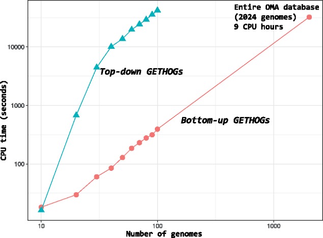
Time performance of GETHOGs algorithm. CPU time to compute the HOGs reconstruction on dataset of different sizes. The timing is recorded on a single instance running on a Intel(R) Xeon(R) CPU E5540 2.53GHz

4 Discussion and conclusion

When compared with other methods, the OMA algorithm has often been reported to be stringent, yielding highly reliable inferences, but suffering from low recall (Altenhoff et al., 2016; Ballesteros and Hormiga, 2016; Trachana et al., 2011). This is certainly true of the ‘OMA groups”, which require fully connected subgraphs of orthologs. For pairs and HOGs, however, we show with this new version that recall can be considerably improved without negatively affecting precision.

Indeed, we introduced multiple improvements to the OMA algorithm, both in the inference of pairwise orthologs and in the inference of HOGs. At the pairwise level, the asymmetric paralogy test increases the number of one-to-many and many-to-many ortholog relationships recovered when the paralogous copies evolve at different rates. Furthermore, the new additivity test reduces errors due to inconsistent distance computations in quartets of sequences (used to infer differential gene losses in the OMA algorithm). These inconsistent distances often arise due to fragmentary sequences, typical of draft-quality genomes.

The improvements in pairwise orthology are not only useful in and of themselves—they directly translate into better HOG inference. Combined with the more scalable and accurate bottom-up GETHOGs, the HOGs inferred by OMA are much more complete, with no or even positive impact on precision.

Some of the ideas underlying these improvements are not new. Methods such as Inparanoid (Remm et al., 2001) or OrthoInspector (Linard et al., 2011) have long been exploiting distances between inparalogs—albeit using alignment score as a proxy—to increase the robustness of one-to-many or many-to-many orthology inference. Likewise, Hieranoid (Schreiber and Sonnhammer, 2013) also infers HOGs in a bottom-up fashion.

However, the distinctive feature of the OMA algorithm has been—and continues to be with this new version—its modular approach, with well-defined and testable objectives at each step of the pipeline (e.g. inference of pairwise orthologs, detection of differential gene losses, inference of HOGs from pairwise orthologs). OMA’s modular approach makes it possible to test and optimize each step in isolation, and to expect an overall improvement when these are combined—as the empirical benchmarks reported above clearly support. In contrast, ad hoc methods can prove difficult to maintain and improve over time, with changes in one part of the pipeline affecting other parts in unexpected ways.

Looking ahead, we see further opportunities for improvement. Unlike pairs and groups in OMA, inference of HOGs strongly relies on knowledge of the species tree. However, many parts of the tree of life remain either poorly resolved or even misleading for some gene families due to incomplete lineage sorting, horizontal gene transfer or hybridization (Philippe et al., 2011). Currently, we collapse branches that are uncertain—however this means that gene duplication occurring within such multi-furcations (i.e. polytomies) confound the HOG inference. Approaches taking a more flexible reading of species phylogeny, such as NOTUNG (Durand et al., 2006) or PHYLDOG (Boussau et al., 2012), may provide a better way forward. We also see considerable potential in exploiting the paralogy graph to further improve HOG inference (Lafond and El-Mabrouk, 2014).

Meanwhile, this OMA 2.0 algorithm is used in the public OMA database from the March 2017 release onwards (Altenhoff et al., 2015; http://omabrowser.org), and can be applied to custom genomes using the open source OMA standalone software version 2.0 (http://omabrowser.org/standalone).

References

- Altenhoff A.M. et al. (2013) Inferring hierarchical orthologous groups from orthologous gene pairs. PLoS One, 8, e53786.. [DOI] [PMC free article] [PubMed] [Google Scholar]
- Altenhoff A.M. et al. (2016) Standardized benchmarking in the quest for orthologs. Nat. Methods, 13, 425–430. [DOI] [PMC free article] [PubMed] [Google Scholar]
- Altenhoff A.M. et al. (2015) The OMA orthology database in 2015: function predictions, better plant support, synteny view and other improvements. Nucleic Acids Res., 43, D240–D249. [DOI] [PMC free article] [PubMed] [Google Scholar]
- Altenhoff A.M., Dessimoz C. (2009) Phylogenetic and functional assessment of orthologs inference projects and methods. PLoS Comput. Biol., 5, e1000262.. [DOI] [PMC free article] [PubMed] [Google Scholar]
- Ballesteros J.A., Hormiga G. (2016) A new orthology assessment method for phylogenomic data: unrooted phylogenetic orthology. Mol. Biol. Evol., 33, 2481. [DOI] [PubMed] [Google Scholar]
- Boeckmann B. et al. (2011) Conceptual framework and pilot study to benchmark phylogenomic databases based on reference gene trees. Brief. Bioinformatics, 12, 423–435. [DOI] [PMC free article] [PubMed] [Google Scholar]
- Boeckmann B. et al. (2015) Quest for orthologs entails quest for tree of life: in search of the gene stream. Genome Biol. Evol., 7, 1988–1999. [DOI] [PMC free article] [PubMed] [Google Scholar]
- Boussau B. et al. (2012) Genome-scale coestimation of species and gene trees. Genome Res., 23, 323–330. [DOI] [PMC free article] [PubMed] [Google Scholar]
- Buneman P. (1974) A note on the metric properties of trees. J. Combin. Theory Ser. B, 17, 48–50. [Google Scholar]
- Cormen T.H. (2009) Introduction to Algorithms MIT Press.
- Dalquen D.A., Dessimoz C. (2013) Bidirectional best hits miss many orthologs in duplication-rich clades such as plants and animals. Genome Biol. Evol., 5, 1800–1806. [DOI] [PMC free article] [PubMed] [Google Scholar]
- Dessimoz C. et al. (2006a) Detecting non-orthology in the COGs database and other approaches grouping orthologs using genome-specific best hits. Nucleic Acids Res., 34, 3309–3316. [DOI] [PMC free article] [PubMed] [Google Scholar]
- Dessimoz C. et al. (2006b) Fast estimation of the difference between two PAM/JTT evolutionary distances in triplets of homologous sequences. BMC Bioinformatics, 7, 529.. [DOI] [PMC free article] [PubMed] [Google Scholar]
- Dessimoz C. et al. (2005) OMA, A comprehensive, automated project for the identification of orthologs from complete genome data: introduction and first achievements In: McLysaght A., Huson D.H. (eds.) RECOMB 2005 Workshop on Comparative Genomics. Springer Berlin Heidelberg, pp. 61–72. [Google Scholar]
- Durand D. et al. (2006) A hybrid micro-macroevolutionary approach to gene tree reconstruction. J. Comput. Biol., 13, 320–335. [DOI] [PubMed] [Google Scholar]
- Fitch W.M. (1970) Distinguishing homologous from analogous proteins. Syst. Zool., 19, 99–113. [PubMed] [Google Scholar]
- Kriventseva E.V. et al. (2008) OrthoDB: the hierarchical catalog of eukaryotic orthologs. Nucleic Acids Res., 36, D271–D275. [DOI] [PMC free article] [PubMed] [Google Scholar]
- Lafond M., El-Mabrouk N. (2014) Orthology and paralogy constraints: satisfiability and consistency. BMC Genomics, 15(Suppl 6), S12.. [DOI] [PMC free article] [PubMed] [Google Scholar]
- Li L. et al. (2003) OrthoMCL: identification of ortholog groups for eukaryotic genomes. Genome Res., 13, 2178–2189. [DOI] [PMC free article] [PubMed] [Google Scholar]
- Linard B. et al. (2011) OrthoInspector: comprehensive orthology analysis and visual exploration. BMC Bioinformatics, 12, 11.. [DOI] [PMC free article] [PubMed] [Google Scholar]
- Overbeek R. et al. (1999) The use of gene clusters to infer functional coupling. Proc. Natl. Acad. Sci. USA, 96, 2896–2901. [DOI] [PMC free article] [PubMed] [Google Scholar]
- Philippe H. et al. (2011) Resolving difficult phylogenetic questions: why more sequences are not enough. PLoS Biol., 9, e1000602.. [DOI] [PMC free article] [PubMed] [Google Scholar]
- Remm M. et al. (2001) Automatic clustering of orthologs and in-paralogs from pairwise species comparisons. J. Mol. Biol., 314, 1041–1052. [DOI] [PubMed] [Google Scholar]
- Roth A.C.J. et al. (2008) Algorithm of OMA for large-scale orthology inference. BMC Bioinformatics, 9, 518.. [DOI] [PMC free article] [PubMed] [Google Scholar]
- Schreiber F., Sonnhammer E.L.L. (2013) Hieranoid: hierarchical orthology inference. J. Mol. Biol., 425, 2072–2081. [DOI] [PubMed] [Google Scholar]
- Smith T.F., Waterman M.S. (1981) Identification of common molecular subsequences. J. Mol. Biol., 147, 195–197. [DOI] [PubMed] [Google Scholar]
- Tatusov R.L. et al. (1997) A genomic perspective on protein families. Science, 278, 631–637. [DOI] [PubMed] [Google Scholar]
- Trachana K. et al. (2011) Orthology prediction methods: a quality assessment using curated protein families. Bioessays, 33, 769–780. [DOI] [PMC free article] [PubMed] [Google Scholar]
- Vilella A.J. et al. (2008) EnsemblCompara GeneTrees: Complete, duplication-aware phylogenetic trees in vertebrates. Genome Res., 19, 327–335. [DOI] [PMC free article] [PubMed] [Google Scholar]