Differential privacy-based evaporative cooling feature selection and classification with relief-F and random forests

Abstract

Motivation

Classification of individuals into disease or clinical categories from high-dimensional biological data with low prediction error is an important challenge of statistical learning in bioinformatics. Feature selection can improve classification accuracy but must be incorporated carefully into cross-validation to avoid overfitting. Recently, feature selection methods based on differential privacy, such as differentially private random forests and reusable holdout sets, have been proposed. However, for domains such as bioinformatics, where the number of features is much larger than the number of observations $p\gg n$, these differential privacy methods are susceptible to overfitting.

Methods

We introduce private Evaporative Cooling, a stochastic privacy-preserving machine learning algorithm that uses Relief-F for feature selection and random forest for privacy preserving classification that also prevents overfitting. We relate the privacy-preserving threshold mechanism to a thermodynamic Maxwell-Boltzmann distribution, where the temperature represents the privacy threshold. We use the thermal statistical physics concept of Evaporative Cooling of atomic gases to perform backward stepwise privacy-preserving feature selection.

Results

On simulated data with main effects and statistical interactions, we compare accuracies on holdout and validation sets for three privacy-preserving methods: the reusable holdout, reusable holdout with random forest, and private Evaporative Cooling, which uses Relief-F feature selection and random forest classification. In simulations where interactions exist between attributes, private Evaporative Cooling provides higher classification accuracy without overfitting based on an independent validation set. In simulations without interactions, thresholdout with random forest and private Evaporative Cooling give comparable accuracies. We also apply these privacy methods to human brain resting-state fMRI data from a study of major depressive disorder.

Availability and implementation

Code available at http://insilico.utulsa.edu/software/privateEC.

Supplementary information

Supplementary data are available at Bioinformatics online.

1 Introduction

In bioinformatics, data exploration is frequently an adaptive and iterative process due to the high dimensionality of the data and large number of features that can be irrelevant to the outcome (e.g. phenotype). When the outcome variable is not used, iterative analysis of the data is not restricted. However, when the outcome variable is used, some penalty must be incurred to limit drawing false conclusions due to chance. For inferential statistics, such as association tests in genome-wide association studies (GWAS), an adjustment for multiple hypothesis testing must be computed to control the false discovery rate (FDR) (Benjamini et al., 2001). For classification analysis, cross-validation (CV) is typically used to estimate the average classification error one would expect to observe in independent data (Hastie et al., 2009). For biological or clinical utility, the goal is to find high accuracy classifiers. Combining feature selection with classification has the advantage of reducing the complexity of classification models while including features that have predictive value. In many cases, the CV error is a biased estimate of the true error rate in independent data, and this risk may increase if feature selection leaks information between folds. Nested CV approaches that integrate feature selection have been used to reduce this type of bias (Varma and Simon, 2006). In addition, bioinformatics data sets, such as gene expression studies, typically have small sample sizes that lead to CV errors with high variance (Simon et al., 2003).

Another approach that was motivated by the concept of differential privacy (Dwork and Roth, 2013) and is suitable for the adaptive nature of many data analyses is the thresholdout algorithm (Dwork et al., 2015), which is applied to data sets with a 2-fold split (training and holdout). Differential privacy was originally developed to mine databases like social networks to learn information about groups while maintaining the privacy of individuals within those groups. This definition quantifies the leaking of each individual’s information as queries are made on the aggregate data. There has been a great deal of research on privacy-preserving data releasing mechanisms (Chen et al., 2009; Fung et al., 2010; Yu and Ji, 2014) after several discussions on the theoretical possibility to identify individuals in GWAS data (Homer et al., 2008; Wang et al., 2009). However, rather than private data release, the current study focuses on developing differential privacy methods to prevent overfitting in statistical data analysis, one of the earliest examples being the thresholdout algorithm.

Thresholdout uses the Laplace mechanism (Dwork, 2006) to maintain differential privacy by ensuring zero information from the holdout set is revealed when the difference of the mean statistic between training and holdout stays within a stochastic threshold. Consequently, by ensuring differential privacy, this reusable-holdout framework keeps the overall statistical estimate stable, and thus allows for generalization, as long as the number of queries remains under the budget which is a function of the size of the holdout set.

As illustrated in Ref. (Dwork et al., 2015), thresholdout incorporates the notion of differential privacy into its feature selection and classification with a 2-fold split (training and holdout), but when selecting relevant features, importance score information is computed from both the training and holdout sets. Here, the thresholdout mechanism is used to prevent leaking of information between training and holdout sets while using both sets to find useful features. Also, we note that their linear classifier simply relies on the sign of the correlation between each attribute and the class labels. In their simulation of partially correlated data (which contains functional attributes), the association with the outcome is created by either adding or subtracting 6 standard deviations from the randomized functional attribute’s values, depending on class label of 1 or –1, respectively. This shift amounts to an effect size that is very large compared to what is found in most bioinformatics data sets. In the current study, we use a different simulation approach with a smaller effect size.

Another distinguishing challenge in bioinformatics is that most data sets contain a small number of observations, $n$, compared to the number of features, $p$. The simulated sample size of 10 000, previously used to test thresholdout, was much larger than most bioinformatics data. In the current study, we simulate data with much smaller sample sizes, in line with bioinformatics data dimensions $n\ll p$. For these smaller sample sizes, thresholdout does preserve privacy, but there is a risk of overfitting the holdout set regardless of the choice of threshold. Thus, we compare each method using data simulations with lower effect sizes and sample sizes as well as complex structures of correlations and interactions among these features.

In our previous work, we developed a backwards elimination feature selection algorithm called Evaporative cooling (EC) that is able to identify relevant features due to main effects and interaction effects (McKinney et al., 2009). Analogous to Evaporative Cooling of an atomic gas, where phase space density is increased through the repeated removal of the most energetic atoms, EC feature selection increases feature space density by iteratively removing the least relevant attributes. The resulting final collection of attributes is then at equilibrium with regard to independent and interaction effects by combining Relief-F and random forest importance scores.

In the current study, we develop a privacy-preserving version of Evaporative Cooling that uses Relief-F for feature selection and random forest for classification with an exponential differential privacy mechanism. Besides the Laplace mechanism, the exponential mechanism is another interesting mechanism that ensures $\epsilon$-differential privacy (McSherry and Talwar, 2007). If $q$ is a quality function that assigns a score to each attribute $a\in A$, and $\Delta q$ is its sensitivity, then the exponential mechanism $M$ that outputs $a$ with probability $\propto \hspace{0.17em}\text{exp}\hspace{0.17em}(\epsilon \hspace{0.17em}q\left(a\right)/2\Delta q)$ maintains $\epsilon$-differential privacy. The focus of the original EC method was on feature selection, rather than classification. The focus of private EC (pEC) is classification but uses feature selection in a way that limits overfitting. We compare pEC and other differentially private algorithms on simulated data with properties typical of bioinformatics. These comparison methods include the original thresholdout algorithm with a linear correlation classifier and a thresholdout algorithm that uses random forest for classification.

The current study is outlined as follows. We first describe the simulation strategy and development of the private Evaporative Cooling algorithm in the Methods section. Through the thermodynamic formalism, we show a relationship between the Maxwell-Boltzmann distribution and differential privacy. We use two main types of simulations to evaluate the methods: data with multiple independent main effects and data with interactions and correlation structure. In the Results section, we investigate the relationship between the simulation parameter $b$ and the detection power obtained by a Welch two-sample t-test as well as Dwork’s simulation effect size parameter referred to as ‘bias’. We also evaluate the accuracy reported by three privacy-preserving algorithms on simulated validation data. The original thresholdout with a linear classifier shows a high degree of overfitting in $n\ll p$ data, which can be ameliorated by using a random forest classifier. In simulated data with characteristics typically seen in bioinformatics, private Evaporative Cooling is shown to not overfit and achieve comparable validation accuracy with thresholdout using random forest when the data contain only main effects of specific attributes and highest accuracy when these attributes interact.

2 Materials and methods

2.1 Simulations

Each simulation consists of two balanced groups of cases and controls with $n=100$ observations for each training, holdout, and testing set. For main effect simulations, we use $p=5\mathrm{000}$ features of which 10% are functional (correlated with class labels). Although this p should be sufficient to compare feature selection and classification algorithms, we also consider the case of 15 000 features, and it is possible to analyze larger data sets. These data dimensions are also comparable to the fMRI data we analyze. The training and holdout sets are used for the thresholdout algorithms, and the testing set is used to determine the true validation accuracy of an algorithm. For each set of simulations parameters, we simulate 100 replicate data sets to assess statistical differences between methods.

2.1.1 Main effect

We employ the linear model used in Ref. (Leek and Storey, 2007):

$$X_{ij}={\beta }_i{y}_j+e_{ij}$$ (1)

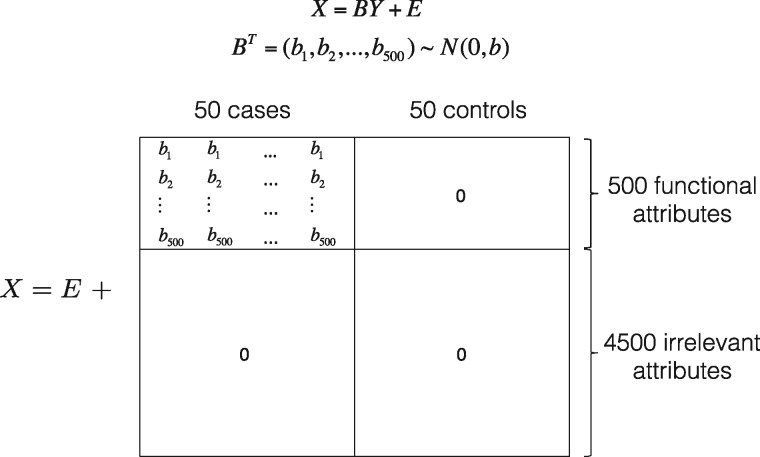
where $X_{ij}$ is the j^th subject’s value of the i^th attribute, ${\beta }_i$ represents the coefficient of the $i^{th}$ attribute, $y_j$ is the biological group (belongs to the set {0,1}) of the observation $j$, and $e_{ij}$ is Gaussian noise with mean 0 and standard deviation 1. A visual representation of the simulation is shown in Figure 1. In this matrix form, $Y=(1,1,\dots ,1,0,0,\dots ,0)$ represents the biological status of 100 samples (50 cases and 50 healthy controls), $B^T=(b_1,b_2,\dots ,b_{500})\sim N(0,b)$ consists of 500 effect sizes, and $E\sim N(0,1)$ adds independent random error to the data.

Fig. 1.

Model matrix of the linear model. The top 500 rows of $BY$ are ‘functional’ attributes that discriminate between the cases and controls. We suppose that, for individuals in the cases group, these attributes’ values are drawn from a normal distribution $N(0,b)$. The effect of $b$ is discussed in the Results section. The matrix $E$ adds independent random errors with mean zero

2.1.2 Interaction effect

We simulate interaction effects by the framework we designed in Ref. (Lareau et al., 2015) for differential co-expression network data. The objective of this framework is to disturb specific attributes’ connections in the co-expression network among the cases only, while leaving the controls’ network untouched. With this goal in mind, we initialize a baseline network of correlations of mean 0 and variance $s_{int}$ between attributes either with uniform random degree distribution (Erdos-Renyi) or scale-free degree distribution. Specifically, if the two attributes $a_1$ and $a_2$ are correlated in the base network, we let $a_{i1}=a_{i2}+{\eta }_i$ for all subjects $i=1,2,\dots ,100$ where ${\eta }_i$ is drawn from N(0, $s_{int}$). Hence, the correlation’s strength is regulated by $s_{int}$: smaller $s_{int}$ yields less noise and hence creates a stronger correlation between the two attributes. After randomly partitioning the samples into groups of cases and controls, we arbitrarily select attributes and permute them within the cases to disrupt the wiring between these target attributes and their neighbors while keeping the group means constant. In other words, we introduce a differential correlation or interaction effect on a subset of co-expressed attributes, even though no main effect will be detected if these attributes are inspected individually (except by chance). The resulting complex network is a realistic representation of gene expression data with differential co-expression effects or resting-state functional magnetic resonance imaging data with differential correlation effects. We remark the stronger the initial correlation (regulated by $s_{int}$) between the target attributes and their neighbors, the more severe the disruption, and thus the stronger interaction effect introduced. This regulation of the effect size is further discussed in the Results section.

2.2 Resting-state functional magnetic resonance imaging (rs-fMRI) data

To test our method on real bioinformatics data, we apply the machine learning classifiers to a human resting-state functional MRI (rs-fMRI) study of major depressive disorder (MDD). Differential connectivity in rs-fMRI networks between cases and healthy controls likely contain important variation that may be used as biomarkers or predictors in diagnostic status (Gotts et al., 2012; Manoliu et al., 2013). The fMRI data include 80 unmedicated MDD (52 females, age ± sd. 33 ± 11) and 80 healthy controls (HCs) (41 females, age ± sd. 31 ± 10). We used AFNI (Cox, 1996) to process the rs-fMRI data and extract 3003 features that are z-transformed correlation coefficients between 78 brain regions identified by a functional region of interest atlas (Shirer et al., 2012) (12 regions of interest in the lower part of cerebellum were excluded due to the limited field of view in our fMRI scan). Two subjects with MDD and one HC were excluded from the analysis due to excessive head motion. To increase power, we only report the prediction accuracy from the holdout set and do not split the data into a third validation set. Specifically, after randomly splitting the entire data in half (training and holdout), we trained the three privacy-preserving algorithms on training data to predict each subject’s diagnostic status (MDD or HC) in the holdout set.

2.3 Algorithms

Using the simulation approach with small effect and sample sizes as well as the rs-fMRI data, we compare the performance of the following algorithms:

1. Original Thresholdout (TO) with Dwork’s linear classifier (Dwork et al., 2015)

2. Random Forest Thresholdout (rfTO), which is TO with the feature selection and classifier replaced with random forest

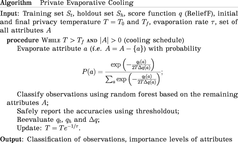
3. Private Evaporative Cooling (pEC) feature selection and classification (Fig. 2)

We note that the second algorithm is almost identical to the first, except that, in place of the simple linear feature selection and classifier, we implement random forest as the feature selection and classifier. The rest of the algorithm, including thresholdout, is kept the same. Within thresholdout, we choose a threshold of $4/\sqrt{n}$ and tolerance of $1/\sqrt{n}$ as suggested in the thresholdout’s supplementary material (Dwork et al., 2015).

Fig. 2.

Pseudocode of private Evaporative Cooling algorithm

2.3.1 Private evaporative cooling (pEC) with relief-F feature selection and random forest classification

In the feature selection piece of this algorithm, the evaporation represents the process of backwards elimination of features, and the temperature $T$ is related to the privacy’s noise parameter (see Fig. 2 for overview). We adapt the idea of the exponential mechanism to iteratively remove features. Particularly, after setting an initial temperature $T_0$ and evaluating $q_t\left(a\right)$, the importance of attribute $a$ from the training set using Relief-F, we allow an attribute to evaporate with a probability proportional to

$$\text{exp}\hspace{0.17em}(-q_t(a)/(2T\Delta q\left(a\right)\left)\right)$$ (2)

where $\Delta q\left(a\right)$ represents the difference of an attribute’s importance score between the holdout, $q_h\left(a\right)$, and training set, $q_t\left(a\right)$:

$$\Delta q\left(a\right)=\left|q_t\right(a)-q_h(a\left)\right|.$$ (3)

Then, at time step $j$, T is decreased according to the following cooling schedule:

$$T=T_0\hspace{0.17em}\text{exp}\hspace{0.17em}(-j/\tau )$$ (4)

with the constant $\tau$ controlling the cooling rate. We note that the formula of relative probability in (2) resembles that of the exponential mechanism and $1/T$ is similar to the privacy loss $\epsilon$ (but not exactly equal to $\epsilon$ because our training and holdout data sets are not adjacent in the privacy sense, and $\Delta q\left(a\right)$ is not the sensitivity of the function $q$). Nevertheless, the parameter $T$ controls the information leak from the holdout set by rescaling the attributes’ importance. The decaying of $T$ in this algorithm is analogous to that of simulated annealing. During the initial cooling steps, simulated annealing algorithms are more tolerant of suboptimal solutions to avoid falling into a local minimum, but as the system cools, simulated annealing algorithms become less tolerant of innovative solutions. Similarly, by putting increasing weight on important attributes, pEC gradually allows for more privacy loss in order to be stricter in selecting potential attributes for removal, thus becoming less likely to remove attributes that have higher training importance score.

We chose Relief-F for the feature selection component because interactions can be an important source of variation in bioinformatics data, and Relief-F has been shown to have high power to identify features that involve complex interactions that are important for distinguishing classes (Draper et al., 2003; Greene et al., 2009; Kononenko, 1994; Kononenko et al., 1997; McKinney et al., 2013; Sikonja and Kononenko, 2003). We chose random forest as the classifier for the pEC algorithm because of its well-known advantages in high dimensional data and wide usage in bioinformatics (Amaratunga et al., 2008; Breiman, 2001). We also use thresholdout as a safe mechanism to output the accuracy obtained from classifying samples in the holdout set.

One other key idea of this algorithm is similar to thresholdout’s: for attributes with the same importance score, pEC prefers to keep attributes with high training-holdout consistency. In other words, the expression in (2) allows an attribute to probabilistically evaporate when it has relatively low ReliefF importance score in training or larger difference in its importance score between the training and holdout set. Also, rewriting this relative probability in (2) gives

$$\text{exp}\hspace{0.17em}(-E(a)/kT)$$ (5)

showing our algorithm’s analogy to the Maxwell-Boltzmann distribution where $E\left(a\right)=q_t\left(a\right)/2\Delta q\left(a\right)$, $k$ is the Boltzman constant, $T$ is the privacy temperature. Note that this Boltzmann scaling can be adapted to any importance score (e.g. random forest permutation score), and the accuracy can be computed by any classifier. The only constraint is that a lower energy represents a lower importance score, which leads to a higher probability of irrelevant features being evaporated.

This distribution considers the probability that a certain attribute is removed from a system as a function of that attribute’s energy and the ‘privacy temperature’ of the system. Writing the differential privacy mechanism as Equation (5) provides a link between what we call the privacy temperature and Jaynes’ maximum information entropy methods (Jaynes, 1957; McKinney et al., 2007).

2.4 Comparison of pEC workflow with a validation workflow

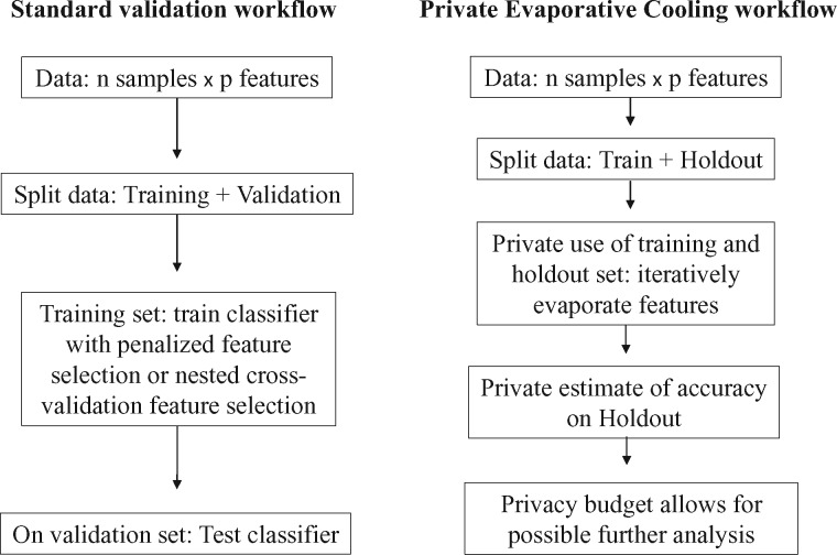
While conducting statistical analyses using the standard workflow is perfectly justified, we present a private workflow with Evaporative Cooling that better utilizes the entire data set. In our example, each workflow includes a training and holdout/validation set. With the validation workflow, because of the small sample size in many bioinformatics studies, setting samples aside for validation may decrease the analysis power significantly. Moreover, once the results from the validation set are released, the validation set cannot be reused in later analyses without introducing bias. With pEC workflow, one can exploit the whole data set and safely adapt the holdout results to later analyses (Fig. 3). Specifically, in pEC workflow, one is able to use the holdout set for feature selection and estimation of accuracy, and the privacy budget allows the analyst to reuse the holdout set.

Fig. 3.

Comparison of pEC workflow with a validation workflow. In each scenario, there is a training set and a data set that is set aside for validation. The pEC mechanism allows the analyst to use the holdout set during feature selection and classification. Privacy also permits reuse of the holdout set

3 Results

3.1 Calibrating the simulation parameters

The average effect size parameter $b$ is the variance in $N(0,b)$ that regulates the strength of the signals in simulations with main effects (Fig. 1). A larger effect size allows for more deviation from the mean of 0 in the group of cases, which in turn increases the proportion of correctly detected attributes in a basic two-sample, unpaired t-test. In order to further examine the meaning of $b$ and compare with the simulation parameter in Dwork’s illustration, we simulate data sets with different values of $b$ with groups of 50 cases and 50 controls for each training, holdout, and validation set. There are 500 functional features out of 5000 total features. We define detection power as the proportion of correctly detected attributes out of the 500 functional ones.

The plots of detection power versus effect size of two different simulations are shown in Figure 4. We first adjust the resulting P-values from a two-sample, unpaired t-test using the Benjamini-Hochberg (FDR) method. We count a discovery when an adjusted P-value is less than the threshold of $\alpha =0.05$. Then, the detection power (true positive rate) is calculated by dividing the number of true discoveries (true functional attributes with small adjusted P-value) by the total number of discoveries. As the effect size increases, the number of correct attributes detected increases, while the false positive rate is controlled at approximately 5%. In terms of precision and recall in information retrieval classification, detection power (vertical axis, Fig. 4) is ultimately the value of recall, and precision is kept at approximately 95% (Supplementary Fig. S1). In the current study, we choose a small effect size of $b=0.4$, which results in about 12% detection power and approximately corresponds with the effect size of 2.3 standard deviations in Dwork’s simulation (solid vertical lines in Fig. 4). We chose this relatively small magnitude to reflect the effect size observed in many real bioinformatics data sets such as gene expression or functional MRI. In contrast, the effect size of 6 standard deviations simulated in Ref. (Dwork et al., 2015) has nearly 100% detection power for an adjusted t-test (dashed vertical line in Fig. 4B). Moreover, we simulate a much smaller, more challenging sample size than that of Dwork’s simulation.

Fig. 4.

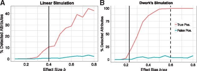
Result of a two-sample, unpaired t-test on simulated data using two simulation methods: Leek’s linear model (left panel) and Dwork’s experiment (right panel). Simulation parameters: 5000 attributes (500 functional) with 50 cases and 50 controls. Note the vertical scales are different. Each point represents the true positive rate (red) and false positive rate (blue) for a simulated data set with the effect size/bias given on the horizontal axis. The true and false percentages were computed based on an adjusted P-value of 0.05. The vertical dash line displays the effect bias used in Dwork’s simulation ($6/\sqrt{n}$). The vertical solid line displays the value of effect size we choose for the linear model simulation and its corresponding bias in Dwork’s simulation that yields the same detection power (∼ 12%) (Color version of this figure is available at Bioinformatics online.)

In the second type of simulation with interaction effects, the parameter that controls effect size is the variance in the added noise term. Smaller variance creates stronger correlation between features, and thus increases the interaction effect. In particular, if $s_{int}$ is very small (e.g. 0.1), the effect size will be very large, which leads to accuracies of almost 1.0 in all methods when a significant number of attributes is included in the model. Similarly, a large value of $s_{int}$ would result in clustering of accuracies at 0.5. These extreme simulation cases with very close accuracy values make it difficult to compare the performance of the different methods. Because of the complex relationship among attributes in this second type, a simple t-test is not helpful in selecting an appropriate variance value. Hence, in this case, we choose a heuristic variance value of $s_{int}=0.4$ that seems to yield intermediate accuracies on the validation sets.

3.2 Comparison of privacy preserving methods

We compare the accuracy of each method for $r=100$ replicate simulated data sets with main effect $b=0.4$ (results in Fig. 5) and interaction effect where $s_{int}=0.4$ (results in Figs. 6, 7). These values of the effect size in the simulations generate adequately challenging data sets so that the methods’ accuracies stay moderate and do not cluster around 0.5 or 1 (too hard or too easy). Each replicate data set is split into training, holdout and validation sets. We make sure that each set has an equal number of cases and controls (50 in each group) to protect the sensitivity to class-label imbalance of the linear classifier in TO. The privacy preserving algorithms are applied to the train and holdout datasets with the holdout accuracy reported (dashed lines), and the trained model is then applied to the independent test data to obtain the true generalization accuracy (solid lines). In all simulations, pEC starts with the initial privacy temperature $T_0=0.1$ that approximately balances the amount of privacy loss and overfitting. The smaller $T_0$, the more initial privacy loss we incur in the pEC algorithm. For example, lowering $T_0$ to 0.05 would likely yield more overfitting on the holdout data due to less stability. Furthermore, to utilize the budget more efficiently, our implementation of pEC removes 50 attributes per iteration. Our main goal is to test the performance of methods to identify features that discriminate between groups and optimize the classification accuracy.

Fig. 5.

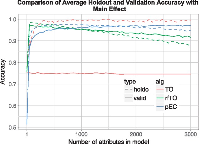
Main effect simulation results. $r=100$ replicate simulations, $n=100$ samples, $d=5000$ attributes, $k=500$ functional attributes, effect size $b=0.4$. Standard thresholdout (TO/red) overfits the independent validation data set; private Evaporative Cooling (pEC/blue) and thresholdout random forest (rfTO/green) give holdout accuracies that are very close to validation accuracies; for reference, standard random forest mean OOB accuracy = 0.832 (Color version of this figure is available at Bioinformatics online.)

Fig. 6.

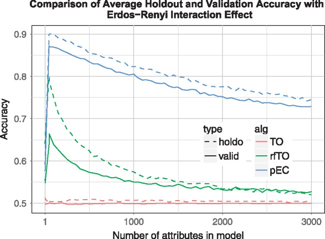
Erdos-Renyi Interaction effect simulation results. $r=100$ replicates, $n=100$ samples, $d=5000$ attributes, $k=500$ functional attributes, effect size $s=0.4$. Standard thresholdout (TO/red) is virtually ineffective (accuracy around 0.5); Private Evaporative Cooling (pEC/blue) yields the best accuracy and prevents overfitting; for reference, standard random forest mean OOB accuracy = 0.736 (Color version of this figure is available at Bioinformatics online.)

Fig. 7.

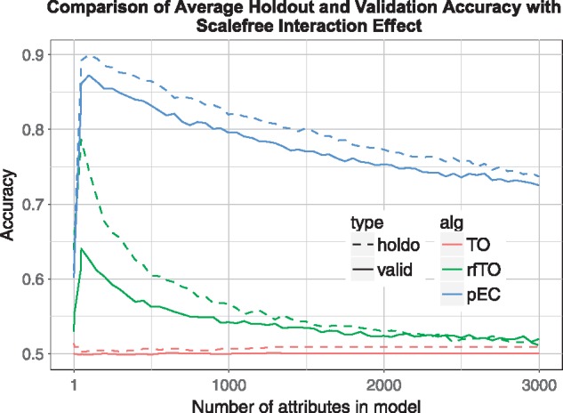
Scale-free Interaction effect simulation results. Comparisons are the same as Figure 6 except the random network has a uniform random degree distribution as opposed to scale free. For reference, standard random forest OOB accuracy = 0.743 (Color version of this figure is available at Bioinformatics online.)

Because of the adaptive attribute evaporation rate, the accuracy values are computed at a different number of attributes across all simulations. To combine the results of 100 simulations, we interpolate the accuracies in each simulation simply with a linear function at all number of attributes, from 1 to 5000. We display the mean interpolated accuracy of each method on 100 simulated data sets.

Besides reporting the accuracy from pEC (blue), rfTO (green) and TO (red), we also report the accuracies from standard random forest (sRF) (ntree = 100) solely as reference accuracies. This average out of bag (OOB) error is computed using the training and holdout data sets combined. It is not proper to compare the output from sRF with other methods because sRF does not consist of any safe-holdout-reuse guarantee that the other methods ensure. In other words, one cannot use sRF’s outcome to make further data-dependent decisions. We still note that in all simulations sRF reports relatively good accuracy and tends to yield the smallest variation in its accuracy.

As we exclude irrelevant attributes (going from right to left in Figs. 5–7), the accuracies of rfTO and pEC increase until too many relevant attributes are removed and the accuracy drops off. For each attribute removal step, the holdout and validation (true) accuracy are very consistent for pEC and rfTO (i.e. they do not overfit). In the interaction case (Figs. 6, 7) rfTO overfits more than pEC when too many attributes are removed. Thresholdout with the linear classifier (TO) significantly overfits for main effect simulations: its holdout accuracy approaches 1.0 as the number of attributes considered increases while its validation accuracy stays around 0.75 (Fig. 5). We believe this overfitting is because of the small number of observations in the data, which is typical of bioinformatics and leads to a reduction in the privacy budget. In simulations with interactions (Figs. 6, 7), although TO does not overfit, it essentially gives null accuracy.

In addition to showing consistent accuracy between holdout and validation sets, pEC and rfTO yield comparable accuracy in main effect simulations (0.9–0.95 across different number of attributes), larger than the accuracy reported by the standard random forest method with 100 trees of 0.832, and much larger than TO’s validation accuracy at approximately 0.75 (Fig. 5). We also remark a slight ‘underfitting’ at the higher numbers of attributes in both rfTO and pEC, which is likely the result of a small pessimistic bias in the out of bag accuracy reported by the random forest classification in both algorithms.

In simulations with interaction effects, the underlying correlation network of attributes uses Erdos-Renyi (Fig. 6) and scale-free (Fig. 7) as base connectivity distributions. When the attributes interact (Figs. 6, 7), pEC outperforms other privacy preserving methods (and even the non-privacy-preserving standard random forest accuracy ∼ 0.74) with better accuracies at all number of selected attributes with peak validation accuracy of 0.87. These patterns hold for larger data sets as well. When the number of variables is increased to 15 000, similar accuracy patterns to Figure 5 are observed in a simulated data set with main effects (results not shown). In an Erdos-Renyi interaction simulation, the pEC algorithm performs similarly as in smaller data sets (Fig. 6). However, rfTO yields lower accuracy when more attributes are added to the data (Supplementary Fig. S2). We believe this decrease is due to the random forest’s independence assumption in the tree node splitting and its underestimation of the interacting attributes’ importance scores when the data contain too many background variables (McKinney et al., 2009).

In fMRI data, pEC and rfTO yield comparable holdout accuracy with maximum accuracies 0.771 (pEC) and 0.743 (rfTO) (Fig. 8). The maximum pEC accuracy uses 52 fMRI connectivities in the model (Supplementary Table S1). Similar to the result in simulations with interaction effects, TO is ineffective, yielding an accuracy of 0.5 at all numbers of connectivity variables. Standard random forest on the entire data set gives an out of bag accuracy of 0.547, which is just slightly above the null accuracy.

Fig. 8.

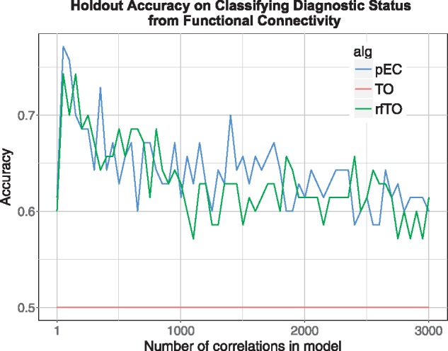
Classification of MDD with rs-fMRI data. Holdout accuracy of the methods on classifying subjects with major depressive disorder (35 in training and 44 in holdout) and healthy control (35 in training and 43 in holdout) status. For reference, the standard random forest OOB accuracy = 0.547 (Color version of this figure is available at Bioinformatics online.)

4 Discussion

Using feature selection to find optimal classification models while controlling overfitting is an important challenge in bioinformatics data due to its large feature space and low sample sizes (Krawczuk and Lukaszuk, 2016). The problem is most severe when a holdout set is not used carefully, such as running feature selection and later classification on the same data set to build models. Differential privacy methods have been recently proposed to deal with feature selection and overfitting. In the current study, we developed a new algorithm called private Evaporative Cooling (pEC) that uses private Relief-F with Evaporative Cooling feature selection as a mechanism for a safe reuse of the holdout set. While simultaneously preventing overfitting, the combination of powerful machine learning methods with Relief-F and random forest provides good prediction accuracy on independent data sets.

We showed that the type of classifier used with the thresholdout algorithm contributes to the degree of overfitting. A simple linear classifier showed very large differences in the holdout and validation accuracy rates, whereas replacing this classifier with random forest and using the same noise and threshold parameters reduces the overfitting to a negligible level. The main reason for this is that the out of bag accuracy which random forest computes from the training set is a reasonable estimate of the generalization accuracy. Hence, even when thresholdout reveals only the training accuracy when this value is close to that from the holdout set, the reported accuracy is a good representation of the predicting accuracy on an independent data set, resulting in no overfitting. Random forest is also better able to handle the smaller effect and sample sizes. pEC, which uses random forests for classification and Relief-F for feature selection, shows negligible overfitting and better validation accuracy than the other thresholdout methods.

In addition to replacing the classification and feature selection components of the original thresholdout algorithm, pEC also involves a simulated annealing-like cooling process of removing irrelevant attributes while maintaining privacy between the training and holdout sets. When interactions exist among attributes, we demonstrated that pEC, among the three comparison methods that include thresholdout, yields the highest validation accuracy and most correctly detected functional attributes (results not shown). In the case of main effect simulations, pEC does not detect the highest number of functional attributes (results not shown); however, its prediction accuracy on validation sets remains higher than the other methods without overfitting.

Evaluating each method’s performance based on selecting features poses a few challenges. In the first simulation with only main effects, because of the randomness generated in the effect size for each ‘functional attribute’, some of the effect sizes could by chance be very small (e.g. on the order of 10⁻⁶) and thus could be masked by the added noise. In other words, some of these intended-to-be-functional attributes can be essentially non-functional and correctly excluded in classification. For the second simulation with interactions, the permutation of attributes within the cases creates a cascading effect. Therefore, the set of functional attributes not only contains these permuted attributes but also their immediate neighbors. Moreover, with the complex structure of the feature’s network, these features have very different weights of importance, which makes it difficult to assess the efficiency in selecting attributes of the algorithms. Thus, we do not compare the algorithms’ feature selection ability in either type of simulation.

We also applied pEC to a real-world fMRI data set and compared its performance with other privacy methods. We demonstrated that pEC gives reliable accuracy and proves to be competitive with private random forest. Among the crucial functional connections in discriminating the diagnostic status, most frequent connections are within the default mode and salience networks and their interactions with other regions (Supplementary Table S1), which is consistent with findings from previous studies (Liang et al., 2013; Sambataro et al., 2014; Yao et al., 2009; Zhu et al., 2012). Moreover, executive control networks are also shown to be part of important connections in distinguishing MDD from HC. Although few resting-state studies have focused on control networks in MDD (Dutta et al., 2014), decreased connectivity between the default mode and executive control networks has been found in patients with MDD (Manoliu et al., 2013; Mulders et al., 2015).

Depending on the goal of an analysis, pEC can be modified with a different set of feature selection and classification techniques other than Relief-F and random forest. The importance score of the attributes $q\left(a\right)$ and the prediction will change according to the new learning methods, but the algorithm’s privacy-preserving ability will remain constant. Moreover, although we illustrated the pEC workflow with a 50–50 2-fold split, one can apply this workflow on an unbalanced split (e.g. 75–25) if one wishes to increase the training set’s size. A current limitation of pEC is the inexact quantification of the amount of privacy loss that results in the choice of the initial privacy temperature. In future work, we plan to use the Boltzmann formalism to develop a mathematical theory mapping pEC’s relationship to the theory of differential privacy and information theory.

The current study focused on quantitative attributes and a categorical response variable. To widen the applicability in bioinformatics, it will be important to implement pEC for regression with quantitative trait data. For categorical predictors, like variants in GWAS, the current pEC method can be directly applied. We also plan to more fully develop a mathematical theory of pEC’s relationship with the theory of differential privacy and information theory.

Funding

This work has been supported in part by NIMH/NIH grants (R01 MH098099 to JB, and K01 MH096175 to WKS). Experimental data were provided by NIMH/NIH grant R01 MH098099 to JB.

Conflict of Interest: none declared.

References

- Amaratunga D. et al. (2008) Enriched random forests. Bioinformatics, 24, 2010–2014. [DOI] [PubMed] [Google Scholar]
- Benjamini Y. et al. (2001) Controlling the false discovery rate in behavior genetics research. Behav. Brain Res., 125, 279–284. [DOI] [PubMed] [Google Scholar]
- Breiman L. (2001) Random forests. Machine Learn., 45, 5–32. [Google Scholar]
- Chen B.C. et al. (2009) Privacy-Preserving Data Publishing. Foundations and Trends in Database. Now Publishers, New York, NY. [Google Scholar]
- Cox R.W. (1996) AFNI: software for analysis and visualization of functional magnetic resonance neuroimages. Comput. Biomed. Res. Int. J., 29, 162–173. [DOI] [PubMed] [Google Scholar]
- Draper B. et al. (2003) Iterative Relief. Conference on Computer Vision and Pattern Recognition Workshop.
- Dutta A. et al. (2014) Resting state networks in major depressive disorder. Psychiatr. Res., 224, 139–151. [DOI] [PubMed] [Google Scholar]
- Dwork C. (2006) Differential Privacy. In, Automata, Languages and Programming, pp. 1–12.
- Dwork C. et al. (2015) STATISTICS. The reusable holdout: preserving validity in adaptive data analysis. Science, 349, 636–638. [DOI] [PubMed] [Google Scholar]
- Dwork C., Roth A. (2013) The algorithmic foundations of differential privacy. Found. Trends® Theor. Comput. Sci., 9, 211–407. [Google Scholar]
- Fung B.C.M. et al. (2010) Privacy-preserving data publishing. Survey Recent Dev. ACM Comput. Surv., 42, 1–53. [Google Scholar]
- Gotts S.J. et al. (2012) Fractionation of social brain circuits in autism spectrum disorders. Brain J. Neurol., 135, 2711–2725. [DOI] [PMC free article] [PubMed] [Google Scholar]
- Greene C.S. et al. (2009) Spatially uniform relieff (SURF) for computationally-efficient filtering of gene-gene interactions. BioData Mining, 2, 5. [DOI] [PMC free article] [PubMed] [Google Scholar]
- Hastie T. et al. (2009) The Elements of Statistical Learning: data Mining, Inference, and Prediction. Springer, New York. [Google Scholar]
- Homer N. et al. (2008) Resolving individuals contributing trace amounts of DNA to highly complex mixtures using high-density SNP genotyping microarrays. PLoS Genet., 4, e1000167. [DOI] [PMC free article] [PubMed] [Google Scholar]
- Jaynes E.T. (1957) Information theory and statistical mechanics. Phys. Rev., 106, 620–630. [Google Scholar]
- Kononenko I. (1994) Estimating attributes: analysis and extensions of RELIEF. Machine Learn. ECML-94 Lecture Notes Comp. Sci., 784, 171–182. [Google Scholar]
- Kononenko I. et al. (1997) Overcoming the myopia of inductive learning algorithms with RELIEFF. Appl. Intel., 7, 39–55. [Google Scholar]
- Krawczuk J., Lukaszuk T. (2016) The feature selection bias problem in relation to high-dimensional gene data. Artif. Intel. Med., 66, 63–71. [DOI] [PubMed] [Google Scholar]
- Lareau C.A. et al. (2015) Differential co-expression network centrality and machine learning feature selection for identifying susceptibility hubs in networks with scale-free structure. BioData Mining, 8, 5. [DOI] [PMC free article] [PubMed] [Google Scholar]
- Leek J.T., Storey J.D. (2007) Capturing heterogeneity in gene expression studies by surrogate variable analysis. PLoS Genet., 3, 1724–1735. [DOI] [PMC free article] [PubMed] [Google Scholar]
- Liang M.J. et al. (2013) Identify changes of brain regional homogeneity in bipolar disorder and unipolar depression using resting-state FMRI. PloS One, 8, e79999. [DOI] [PMC free article] [PubMed] [Google Scholar]
- Manoliu A. et al. (2013) Insular dysfunction within the salience network is associated with severity of symptoms and aberrant inter-network connectivity in major depressive disorder. Front. Human Neurosci., 7, 930.. [DOI] [PMC free article] [PubMed] [Google Scholar]
- McKinney B.A. et al. (2009) Capturing the spectrum of interaction effects in genetic association studies by simulated evaporative cooling network analysis. PLoS Genet., 5, e1000432. [DOI] [PMC free article] [PubMed] [Google Scholar]
- McKinney B.A. et al. (2007) Evaporative cooling feature selection for genotypic data involving interactions. Bioinformatics, 23, 2113–2120. [DOI] [PMC free article] [PubMed] [Google Scholar]
- McKinney B.A. et al. (2013) ReliefSeq: a gene-wise adaptive-K nearest-neighbor feature selection tool for finding gene-gene interactions and main effects in mRNA-Seq gene expression data. PloS One, 8, e81527. [DOI] [PMC free article] [PubMed] [Google Scholar]
- McSherry F., Talwar K. (2007) Mechanism design via differential privacy. In: 48th Annual IEEE Symposium on Foundations of Computer Science (FOCS'07), IEEE Computer Society, Providence, RI. pp. 94–103.
- Mulders P.C. et al. (2015) Resting-state functional connectivity in major depressive disorder: a review. Neurosci. Biobehav. Rev., 56, 330–344. [DOI] [PubMed] [Google Scholar]
- Sambataro F. et al. (2014) Revisiting default mode network function in major depression: evidence for disrupted subsystem connectivity. Psychol. Med., 44, 2041–2051. [DOI] [PubMed] [Google Scholar]
- Shirer W.R. et al. (2012) Decoding subject-driven cognitive states with whole-brain connectivity patterns. Cereb. Cortex, 22, 158–165. [DOI] [PMC free article] [PubMed] [Google Scholar]
- Sikonja M.R., Kononenko I. (2003) Theoretical and empirical analysis of ReliefF and RReliefF. Machine Learn., 53, 23–69. [Google Scholar]
- Simon R. et al. (2003) Pitfalls in the use of DNA microarray data for diagnostic and prognostic classification. J. Natl. Cancer Inst., 95, 14–18. [DOI] [PubMed] [Google Scholar]
- Varma S., Simon R. (2006) Bias in error estimation when using cross-validation for model selection. BMC Bioinform., 7, 91. [DOI] [PMC free article] [PubMed] [Google Scholar]
- Wang R. et al. (2009) Learning your identity and disease from research papers: information leaks in genome wide association study In: Proceedings of the 16th ACM Conference on Computer and Communications Security. ACM, Chicago, Illinois, USA, pp. 534–544. [Google Scholar]
- Yao Z. et al. (2009) Regional homogeneity in depression and its relationship with separate depressive symptom clusters: a resting-state fMRI study. J. Affect. Disorders, 115, 430–438. [DOI] [PubMed] [Google Scholar]
- Yu F., Ji Z. (2014) Scalable privacy-preserving data sharing methodology for genome-wide association studies: an application to iDASH healthcare privacy protection challenge. BMC Med. Inform. Decision Making, 14 (Suppl 1), S3. [DOI] [PMC free article] [PubMed] [Google Scholar]
- Zhu X. et al. (2012) Evidence of a dissociation pattern in resting-state default mode network connectivity in first-episode, treatment-naive major depression patients. Biol. Psychiatr., 71, 611–617. [DOI] [PubMed] [Google Scholar]
Associated Data
This section collects any data citations, data availability statements, or supplementary materials included in this article.