Integrative deep models for alternative splicing

Abstract

Motivation

Advancements in sequencing technologies have highlighted the role of alternative splicing (AS) in increasing transcriptome complexity. This role of AS, combined with the relation of aberrant splicing to malignant states, motivated two streams of research, experimental and computational. The first involves a myriad of techniques such as RNA-Seq and CLIP-Seq to identify splicing regulators and their putative targets. The second involves probabilistic models, also known as splicing codes, which infer regulatory mechanisms and predict splicing outcome directly from genomic sequence. To date, these models have utilized only expression data. In this work, we address two related challenges: Can we improve on previous models for AS outcome prediction and can we integrate additional sources of data to improve predictions for AS regulatory factors.

Results

We perform a detailed comparison of two previous modeling approaches, Bayesian and Deep Neural networks, dissecting the confounding effects of datasets and target functions. We then develop a new target function for AS prediction in exon skipping events and show it significantly improves model accuracy. Next, we develop a modeling framework that leverages transfer learning to incorporate CLIP-Seq, knockdown and over expression experiments, which are inherently noisy and suffer from missing values. Using several datasets involving key splice factors in mouse brain, muscle and heart we demonstrate both the prediction improvements and biological insights offered by our new models. Overall, the framework we propose offers a scalable integrative solution to improve splicing code modeling as vast amounts of relevant genomic data become available.

Availability and implementation

Code and data available at: majiq.biociphers.org/jha_et_al_2017/

Supplementary information

Supplementary data are available at Bioinformatics online.

1 Introduction

A key contributor to transcriptome complexity is alternative splicing (AS): the joining together of different exonic segments of a pre-mRNA to yield different gene isoforms. The most common type of AS event in human and mouse is exon skipping where a fraction of the mRNA produced include an exon while others skip it. Thousands of such variations were found to be highly conserved and common between tissues. Overall, more than 90% of human multi-exon genes are alternatively spliced (Pan et al., 2008; Wang et al., 2008) and splicing defects have been associated with numerous diseases. This has motivated detailed studies of AS variations across tissues, development stages and malignant states (Scotti and Swanson, 2016). These studies monitor mRNA expression at exonic resolution using RNA-Seq in a variety of experimental conditions, including knockdown (KD), knockout (KO) or over-expression (OE) of condition specific splicing factors (SF). Other experiments monitor binding affinity of splice factors using several similar protocols involving UV cross-linking of the factor to the RNA, followed by immunoprecipitation and sequencing of the bound RNA fragments (CLIP-Seq).

In parallel, the fact that splicing outcome is highly condition specific and regulated by many factors led to an effort to computationally derive predictive ‘splicing codes’: models that use putative regulatory features (e.g. sequence motifs, secondary structure) to predict splicing outcome in a condition specific manner (e.g. brain tissue; Barash et al., 2010a; Barash et al., 2010b). Concentrating on cassette exons, the most common form of AS in mammals, these models aimed to predict percent splicing inclusion (PSI, $\Psi$) of the alternative exon, or changes of its inclusion (dPSI, $\Delta \Psi$). Such models have been used successfully to identify novel regulators of key genes in disease associated genes, and predict the effect of genetic variations on splicing outcome (Gazzara et al., 2014; Xiong et al., 2015; Sotillo et al., 2015). However, given the sharp growth in sequencing data, two main questions are: Can we leverage the new CLIP-Seq and splice factors KD/OE experiments and more generally, can we improve on current splicing code models?

Previous work has shown that Bayesian Neural Networks compare favorably to a plethora of other modeling approaches including K-Nearest Neighbors, Support Vector Machine, Naive Bayes and Deep Neural Networks with dropouts (Xiong et al., 2011; Srivastava et al., 2014). Specifically, (Srivastava et al., 2014) described dropout as performing an approximation to the BNN Bayesian model averaging, and pointed to the latter as being advantageous for smaller datasets. However, later work using a Deep Neural Network with an autoencoder demonstrated improved performance compared to a BNN model (Leung et al., 2014). Notably, these different works used different datasets and mixed the effect of modeling framework (BNN versus DNN) with changes of the target function. Thus, in this work we reconstructed previous BNN and DNN models on the original dataset from (Leung et al., 2014) to establish a baseline. Afterwards, we monitored the effect of a new target function, of increasing dataset size by exploiting improvements in RNA-Seq quantification algorithms (Vaquero-Garcia et al., 2016), and adding new types of experimental data.

The first contribution of this work is in developing a new target function for splicing code models. Due to limitations of both available data and algorithms, previous works were unable to predict $\Psi$ or $\Delta \Psi$ directly. Instead, they formulated a three way prediction task $\left\{p_{t,e}^s\right|0\le p_{t,e}^s\le 1,\sum _s{p}_{t,e}^s=1\}$ for any exon e in each condition t. In the original formulation, s represented the chances for increased inclusion, exclusion or no change for exon e in condition t, compared to a hidden baseline of inclusion inferred from a set of 27 tissues (Barash et al., 2010a). This formulation allowed the learned model to concentrate its predictive power on tissue regulated exons, using a dedicated sparse factor analysis model to identify those exons from noisy micro-array data (Barash et al., 2010b). Subsequently, the same target function formulation was used, but instead of inferring splicing changes, s now represented binning of $\Psi$ values into three levels: ‘Low’ ($0\le \Psi <33\%$), ‘Medium’ ($33\%\le \Psi <66\%$) and ‘High’ ($66\%\le \Psi \le 100\%$). While useful, these target functions are inherently unsatisfying as an approximation to the underlying biological variability. Here, we develop a new target function which models $\Psi$ directly, and demonstrate its improved accuracy compared to previous approaches. Serving as a baseline, Figure 1 depicts the improvement in percent variance explained in $\Psi$ by the new model compared to previous BNN and DNN on the original dataset used by (Leung et al., 2014).

Fig. 1.

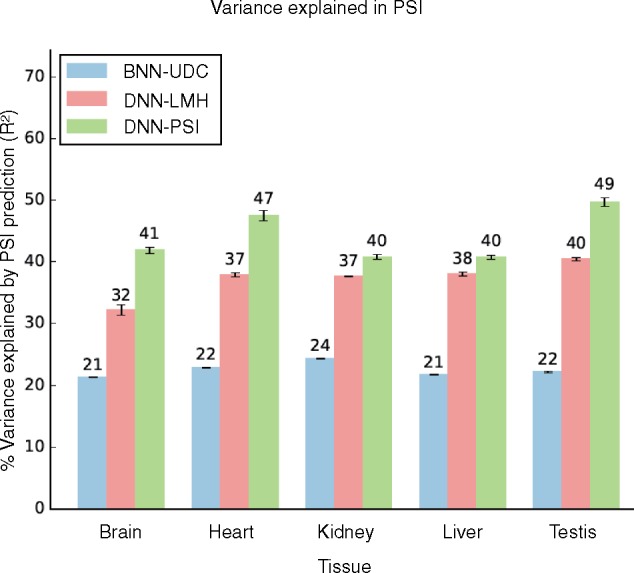
Improvement in percent variance explained by the new target function (green bars) compared to previous BNN (blue bars) and DNN (red bars) models on the tissue data used by (Leung et al., 2014)

The second contribution of this work is developing a framework to integrate additional types of experimental data into the splicing code models. Specifically, CLIP-Seq based measurements of in vivo splice factors binding are turned into an additional set of input features while knockdown and over-expression experiments are added with binary vectors coding the tissue and splice factor (if any) measured. A graphical representation of the old and the new model architectures is given in Figure 2. We demonstrate the effect of the new integrative modeling approach using a set of CLIP-Seq, knockdown and overexpression experiments for members of the RBFOX, CELF and MBNL family of splicing factors in mouse heart, muscle and brain. Finally, we showcase some of the possible biological usage cases for these splicing code models for accurate in silico prediction of splice factor KO effect, and for identifying novel regulatory interplay between different splice factors.

Fig. 2.

Architecture of the Bayesian Neural Network, Deep Neural Network used by (Leung et al., 2014) referred as Leung’s Deep Neural Network, new Deep Neural Network models for tissue data and for splice factor Knockdown/Overexpression data. Green represents new features added to the existing models

2 Materials and methods

2.1 Datasets

Two RNA-Seq datasets were processed for this work. One, denoted Five Tissue Data, is the RNA-Seq data from five mouse tissues (brain, heart, kidney, liver and testis) produced by (Brawand et al., 2011). This dataset was used in the (Leung et al., 2014) paper and thus to ensure that we can accurately reconstruct their models, we use it to compare the old and new models. We generated genomic features and PSI quantification for ∼12 000 cassette exons used in (Barash et al., 2013) for this dataset for the five tissues using MAJIQ (Vaquero-Garcia et al., 2016) and AVISPA (Barash et al., 2013). The second dataset, denoted MGP Data, was prepared by (Keane et al., 2011) and it contains RNA-Seq data from six tissues (heart, hippocampus, liver, lung, spleen and thymus) with average read coverage of 60 million reads. To this data we added 15 CLIP-Seq experiments (see Supplementary Table S10). Together, these datasets highlight some of the challenges involved in utilizing such diverse experiments. First, CLIP-Seq experiments give noisy measurement of where a splice factor binds. The measurements are noisy since binding signal (reads aligning to a certain area) may be false positives, may not indicate active regulation and may suffer from false negatives due to low coverage, indirect binding, antibody sensitivity, etc. Moreover, these experiments are typically executed by different labs, in different conditions and at varying levels of coverage. Thus, it is crucial that any learning framework that we develop should be able to handle missing and noisy measurements.

In our learning setting, the CLIP-Seq data is turned to input features indicating possible binding in a region proximal to the alternative exon (e.g. upstream intron). Since CLIP-Seq measurements are inherently noisy and suffer from different coverage levels we abstract them as binary indicators of binding in the various regions of interest around our alternative cassette exons. The target in our problem formulation is the relative exon inclusion level in a given experiment, expressed as percent spliced in (PSI, $\Psi \in [0,1]$). $\Psi$ serves to capture the proportion of isoforms that include the alternative cassette exon versus those that skip it. But since these are not observed directly, the short sequencing reads are used to estimate these values. Specifically, we apply MAJIQ (Vaquero-Garcia et al., 2016) to derive posterior distribution over $\Psi \in [0,1]$ using the short sequencing reads. Similarly, when comparing two conditions the short reads are used to construct a posterior distribution over dPSI $\Delta \Psi \in [-1,1]$ for the inclusion of the alternative exon. In practice many alternative exons tend to be either highly included or highly excluded in any given condition, but around 20% of the measurements in our dataset have $0.1<E[\Psi ]<0.9$ and the concentration of the posterior $\Psi$ or $\Delta \Psi$ distribution around that mean value depends on the total number of reads hitting that region and how these are distributed across the transcriptome (Vaquero-Garcia et al., 2016).

Except the additional CLIP based features described above, we derived a feature set similar to previous works, to enable comparison. The 1357 non CLIP-Seq features are comprised of binary, integer and real valued features. These features have vastly different distributions with some being highly sparse, and some features being highly correlated (e.g. alternative representations of a splice factor binding motif). Finally, in any given condition only a small subset of those features are expected to represent relevant regulatory features.

Since many splicing changes occur in complex/non-binary splicing events, limiting the splicing code model to the original predefined 12 000 cassette events means that we may lose many important splicing variations. To capture additional cassette or cassette-like splicing variations we develop a pipeline that parses gene splice graphs constructed by MAJIQ to find additional training samples in the dataset. This process allowed us to find 2876 more events changing in at least one tissue in the MGP data.

Next, we process seven splice factor knockdown, knockout and over-expression RNA-Seq datasets for four key splicing factors CELF1/2, MBNL1 and RBFOX2 (for details of the datasets, see Supplementary Table S11). These datasets pose a challenge for any integrative learning framework since they are low coverage, noisy and are processed by different labs.

We divided our datasets into 5-folds. 3-folds were used for training, one was used for validation and the last one was used for testing. We repeated the modeling tasks three times, permuting the dataset each time to produce standard deviation estimates for performance evaluation.

2.2 Likelihood target function

Motivated by the high noise in microarrays and later applied to RNA-Seq data, previous works translated the measurements of exon inclusion levels into a posterior distribution over random variable $q_{c,s}^e$ for each exon e and condition c with three possible assignments $\left\{q_{c,s}^e\right\}$ where $q_{c,s}^e\ge 0 \forall e,c,s$ and $\sum _s{q}_{c,s}^e=1$. For PSI prediction, $s\in \{L,M,H\}$ represent chances of $0\le \Psi <0.33,\hspace{0.17em}0.33\le \Psi <0.66$ and $0.66\le \Psi \le 1$, respectively. For changes in PSI, $s\in \{inc,exc,nc\}$, represent chances of increased inclusion, exclusion or no change. Consequently, an information theoretic code quality measure $({\mathcal{Q}}_c)$ was used to score the predictions made by the splicing code. ${\mathcal{Q}}_c$ is expressed as the difference in the Kullback–Leibler (KL) divergence between each target and predicted distribution:

$$\begin{array}{c}{\mathcal{Q}}_c=\sum _{e=1}^E{D}_{KL}(q_c^e||\overline{q})-D_{KL}(q_c^e||p_c^e)\hfill \\ =\sum _{e=1}^E\sum _{s\in \{inc,exc,nc\}}{q}_{c,s}^e\hspace{0.17em}\text{log}\hspace{0.17em}\left(\frac{p_{c,s}^e}{{\overline{q}}_s}\right),\hfill \end{array}$$ (1)

where c is the splicing condition (e.g. CNS), E is the number of exons and $p_{c,s}^e$ and $q_{c,s}^e$ are the predicted and target probabilities. Alternatively, ${\mathcal{Q}}_c$ can be interpreted as the log-likelihood of the predictions minus the log-likelihood of a naive predictor based on the marginal distribution only.

Although useful, this target function suffers from several deficiencies when applied to RNA-Seq data. First, the binning results in a rudimentary estimation of $\Psi$ and $\Delta \Psi$. Second, the optimization only aims to bring $p_{c,s}^e$ and $q_{c,s}^e$ closer, without any relation to order or meaning. For example, if a cassette event has low inclusion ($q_{c,s=L}\sim 1$) then predicting $p_{c,s=M}\sim 1$ or $p_{c,s=H}\sim 1$ are just as bad. Moreover, in cases where an event suffers from insufficient or highly variable read coverage we may have $q_{c,s=L}\sim q_{c,s=M}\sim q_{c,s=H}$. In such cases, a model with prediction $p_{c,s=H}\sim 1$ based on sequence features will be penalized, even though there was no substantial evidence against it.

In order to overcome the above limitations, for every pair of conditions c and $c^{\prime }$, we define three target variables as:

$$\begin{array}{c}{T}_{{\Psi }_{e,c}}=E[{\Psi }_{e,c}]\hfill \\ T_{\Delta {\Psi }_{inc,c,c^{\prime }}}=|\max (\mathrm{ϵ},E[\Delta {\Psi }_{c,c^{\prime }}])|\hfill \\ T_{\Delta {\Psi }_{exc,c,c^{\prime }}}=|\min (\mathrm{ϵ},E[\Delta {\Psi }_{c,c^{\prime }}])|\hfill \end{array}$$ (2)

where $T_{{\Psi }_{e,c}}$ is the expected PSI value of the event e in condition c, $T_{\Delta {\Psi }_{inc,c,c^{\prime }}}$ captures the dPSI for events with increased inclusion between condition c and $c^{\prime }$ and $T_{\Delta {\Psi }_{exc,c,c^{\prime }}}$ captures the dPSI for events with increased exclusion between condition c and $c^{\prime }$. $\mathrm{ϵ}$ is a uniform random variable with values between 0.01 and 0.03, it is used to provide very low dPSI values for non-changing events. $E[{\Psi }_c]$ and $E[\Delta {\Psi }_{c,c^{\prime }}]$ were computed from the raw RNA-Seq data from condition c and $c^{\prime }$ using MAJIQ (Vaquero-Garcia et al., 2016). Given the above target variable definitions, we define the new likelihood target function as:

$$\begin{array}{c}\mathcal{L}=\sum _c\sum _e^E{k}_{c,e}{w}_{c,e}\sum _t{\mathcal{L}}_{t,c,e}\hfill \\ {\mathcal{L}}_{t,c,e}=t\hspace{0.17em}\text{log}\hspace{0.17em}\widehat{t}+(1-t)\hspace{0.17em}\text{log}\hspace{0.17em}(1-\widehat{t})\hfill \\ w_{c,e}=\sum _{\Psi =E[{\Psi }_{e,c}]-\Delta }^{E[{\Psi }_{e,c}]+\Delta }P(\Psi )\hfill \end{array}$$ (3)

where $t\in \{T_{{\Psi }_{e,c}},T_{\Delta {\Psi }_{inc,c,c^{\prime }}},T_{\Delta {\Psi }_{exc,c,c^{\prime }}}\}$ and $k_{c,e}=1$ if exon e is quantifiable in condition c. The weight $w_{c,e}$ is defined by the probability mass in an area $\pm \Delta$ around the expected ${\Psi }_c$ as defined by MAJIQ. This definition carries several benefits. First, it allows us to combine many different datasets, where the same event may or may not be quantifiable. Second, even when an event is deemed quantifiable ($k_{c,e}=1$), the model can take into account the confidence of MAJIQ in the $\Psi$ inferred from the RNA-Seq experiment based on the number of reads encountered for the event.

2.3 Models

2.3.1 Architecture

The BNN model was described in detail in (Xiong et al., 2011; Leung et al., 2014). Briefly, the network consists of one hidden layer with varying number of sigmoidal hidden units. Network weights are random variables with a Gaussian distribution and a spike and slab prior which encourages sparsity. Figure 2 shows the network architecture of the BNN used in this work. Notably, (Leung et al., 2014) only used the Low, Medium and High PSI variables for the BNN, which may limit the model’s ability to learn splicing change between tissues. For example, if we have an alternative cassette exon e in conditions c and $c^{\prime }$ s.t. ${\Psi }_{e,c}\sim 0.1$ and ${\Psi }_{e,c^{\prime }}\sim 0.3$ with high confidence, the splicing change for exon e between condition c and $c^{\prime },\hspace{0.17em}\Delta {\Psi }_{e,c,c^{\prime }}\sim -0.20$, is considered significant in the field. However, if we translate these PSI values to LMH variables, both ${\Psi }_{e,c}$ and ${\Psi }_{e,c^{\prime }}$ will be in the Low category ($0\le \Psi <0.33$) and the model will not be able to learn the splicing change. We therefore supplemented the LMH variables with UDC variables for inclusion level going up, down or not changing. This addition made the BNN targets equivalent to those of the DNN architecture used in that work, leading to improved performance for the BNN model (see Supplementary Table S4).

The original DNN model shown in Figure 2 included an autoencoder layer with tanh activation and two hidden layers with ReLU activation units. Additionally tissue type was input as two hot vectors of length equal to the number of tissues in the dataset where each bit represents a tissue and is active when the network is input an event comparing that tissue with another. For example, if the tissue order is [brain, heart, kidney, liver and testis] and the current comparison is brain versus heart, then the two tissue type hot vectors will be [10000] and [01000]. Dropout with probability 0.5 was used in each layer except the autoencoder layer. The hyperparameters are described in Supplementary Table S12. We experimented with different types of network architectures with different number of hidden layers and hidden units, different activation units and batch normalization. Since none of those architectures performed significantly better (data not shown) we decided to maintain the original DNN architecture for the purpose of this work.

The new DNN model architecture shown in Figure 2 includes the following additions. First, the target function has been changed as described in Section 2. We also added 874 CLIP features to the input dataset. We maintained the three layer structure of the original DNN models since we observed that adding additional layers did not improve performance. Dropout with probability 0.5 was applied to the second and third layers. We noticed that adding L1/L2-regularization did not have any impact on the model performance and we decided to exclude it from the final model. We allowed the learning rates of the three target variables to vary to capture optimal model performance.

As shown in Figure 2, for splice factor modeling, we modified the tissue type input to include the splice factor knockdown/knockout or overexpression data. We used two hot vectors with length equal to the number of tissues to represent the tissues and two hot vectors with length equal to the number of splice factors to represent the splice factors. Since the datasets for this model were lower coverage and more noisy than the previous models, this model was more sensitive to different hyperparameter values during the tuning phase. Three hidden layers were found to be optimal and L1-regularization was performed on the autoencoder layer. Dropout of 0.5 was used for the second and third hidden layers.

2.3.2 Learning

Following the procedure suggested by (Leung et al., 2014), we trained the first layer of the model as an autoencoder for dimensionality reduction. This procedure proved beneficial for the new models as well. Next, the set of weights from the first layer were fixed and the tissue input was added. In the second stage, the two layered feed forward neural network was trained using SGD with momentum, and weights were fine tuned by backpropagation. Each sample input to the network consists of 1357 genomic (and 874 CLIP) features and has three target variables, $T_{{\Psi }_{e,c}}$, $T_{\Delta {\Psi }_{inc,c,c^{\prime }}}$ and $T_{\Delta {\Psi }_{exc,c,c^{\prime }}}$. Training batches are biased to prioritize changing events. Early stopping and dropout layers prevent the network from overfitting.

Our target variables capture different aspects of splicing change, one learns the baseline PSI for an event in a condition and the other two learn the inclusion and exclusion dPSI of that event between conditions. Therefore varying their learning rates improved overall model performance. The autoencoder network was trained for 300–500 epochs and the feed-forward neural network was trained for 1000–1500 epochs. Validation data was used for the hyperparameter tuning, and once the set of hyper parameters were fixed, the final model was trained with the training and the validation data. 15 models were trained with the 5-folds and three permutations of the whole datasets. The performance evaluation is on the concatenated predictions of the test set from the 5-folds and error bars are computed using the three permutations. Tensorflow was used to develop the deep model and GPUs were used to accelerate the training process.

For the BNN model, each tissue pair was trained as an independent model. Spike and slab prior was used to enforce sparsity and the weights were assumed to have an Gaussian distribution. 950 samples from the posterior distribution of weights were generated using 1000 MCMC training iterations with Gibbs sampling. Initial 50 samples were discarded as burn-in. The final predictions are generated by averaging over the predictions from the 950 sampled weights. 15 models were trained per tissue comparison with 5-fold cross validation and three data permutations. After fixing the model hyperparameters, the validation data was included in the training of the final model.

3 Results

For assessing the prediction accuracy, two types of measures have been used in this work. The predicted $E[{\widehat{\Psi }}_{c,e}]$ is compared to the estimated $E[{\Psi }_{c,e}]$ from the RNA-Seq experiments to compute the fraction of variance explained (R²). Area under the ROC curve (AUC) was computed for the prediction of exons that were differentially excluded/included ($|\Delta {\Psi }_{e,c,c^{\prime }}|\ge 0.15$) or not changing ($|\Delta {\Psi }_{e,c,c^{\prime }}|\le 0.05$).

We aim to measure the effect of each new element on the prediction accuracy. As a baseline, Figure 1 shows the effect of new target function on prediction accuracy when the models are trained on the original dataset used by (Leung et al., 2014) and no other modeling additions are made. We see significant improvement (5–22.5%) in PSI estimation and in splicing target prediction (see Supplementary Table S6) by the new model (DNN-PSI) when compared to the DNN (DNN-LMH) and BNN (BNN-UDC) with the old target function. We note that the results for the previous models are not directly extracted from (Leung et al., 2014), but rather reconstructed to produce similar performance since both code and data were not available in the original publication. Supplementary Figure S2 shows a scatter-plot comparing the performance (AUC-ROC) reported in (Leung et al., 2014) on x-axis and our reconstruction on y-axis. This figure shows that despite different RNA-quantification procedures and data selection criteria, our reconstruction has comparable performance to the (Leung et al., 2014) model. In fact, our model performs better on the Medium class ($0.33\le \Psi <0.66$) of PSI quantification where generally a higher proportion of differential splicing events are located. We added inclusion, exclusion and no change output variables to the Bayesian Neural Network since it improved splicing target prediction performance when compared to the BNN without these labels [BNN-MLR, Leung et al. (2014); see Supplementary Table S4]. DNN-LMH was designed according to the architecture and hyperparameters described in Leung et al. (2014). Also, since the DNN-LMH does not predict PSI directly, we computed the $E[\Psi ]$ as the weighted average of the {L, M, H} class prediction probabilities, following (Xiong et al., 2015).

As noted earlier, previous works (Barash et al., 2013; Leung et al., 2014; Xiong et al., 2015) were performed on a predefined set of ∼12 000 alternative cassette exons. This approach of using only predefined cassette exons can limit the performance of the learned models, especially those involving deep neural networks which require large datasets. Thus, we developed a process termed cassettization (see Section 2.1) to detect and quantify additional cassette and cassette like alternative exons from RNA-Seq data. Additionally, due to the limited coverage of (Brawand et al., 2011), we performed subsequent analysis on the MGP data described in Section 2.1. To assess the effect of cassettization on performance, we used two identically configured BNN models and trained one on the original 12 000 cassette exons (BNN-UDC) while the second (BNN-CAS) got additional training data with cassettized events not present in the original dataset. Figure 3a shows that cassettization caused a substantial improvement in PSI estimation and splicing target prediction (see Supplementary Table S7) with all other factors being constant.

Fig. 3.

(a) Effect of different elements on PSI estimation (% variance explained) (a) Increasing original dataset size by using cassettization (see Section 2.1, BNN-UDC (blue) versus BNN-CAS (brown). BNN-UDC: Bayesian Neural Network with Up, down, no change target variables and old target function; BNN-CAS: BNN-UDC with cassettized data) (b) Adding CLIP data (BNN-CAS (brown) versus BNN-CAS-CLIP (purple). BNN-CAS-CLIP: BNN-CAS with CLIP data). (c) Overall effect of new target function and Deep Neural Network on PSI estimation measured by comparing BNN-CAS-CLIP (purple, BNN with cassettization, CLIP data and the old target function) and DNN-PSI-CAS-CLIP (green, DNN with cassettization, CLIP data and the new target function)

Our next goal was to measure the effect of CLIP-Seq data on PSI estimation. Using the same setup described above, we trained two BNNs identical in every aspect except that one was given the CLIP data as input features (BNN-CAS-CLIP) and the other (BNN-CAS) was not. Introducing the CLIP features added a modest improvement to the PSI estimation as seen in Figure 3b. One possible explanation for the modest improvement could be underfitting of BNN-CAS-CLIP since CLIP was introduced as new features to the model but the model’s hidden layer size and other hyperparameters were fixed.

In order to test the combined effect of the new target function, CLIP data and cassettization on the model’s performance and to compare BNN and DNN frameworks for the task of PSI estimation, we trained a BNN model with the old target function, cassettization and CLIP (BNN-CAS-CLIP) and a DNN model with the new target function, cassettization and CLIP (DNN-PSI-CAS-CLIP). Figure 3c and Table 1 summarize the results for the two models for both PSI estimation and splicing target prediction. Figure 3c shows large performance improvement by the new model for PSI estimation when compared to the BNN. This improvement carries over to the task of splicing target prediction for every tissue pair seen in Table 1.

Table 1.

Comparison of splicing target prediction of DNN-PSI-CAS-CLIP versus BNN-CAS-CLIP in terms of AUC of Inclusion versus not-Inclusion, Exclusion versus not-Exclusion and Change versus not-Change

Tissue pair	Model	Inclusion	Exclusion	No change
Heart-Hipp	BNN-CAS-CLIP	92.97 ± 0.12	88.22 ± 0.16	92.26 ± 0.06
	DNN-PSI-CAS-CLIP	95.70 ± 0.06	94.09 ± 0.34	94.72 ± 0.06
Heart-Liver	BNN-CAS-CLIP	78.09 ± 0.49	89.38 ± 0.24	85.13 ± 0.15
	DNN-PSI-CAS-CLIP	92.15 ± 0.60	96.26 ± 0.18	94.11 ± 0.26
Heart-Lung	BNN-CAS-CLIP	82.52 ± 0.67	89.77 ± 0.18	87.94 ± 0.18
	DNN-PSI-CAS-CLIP	92.15 ± 0.80	95.42 ± 0.30	93.60 ± 0.26
Heart-Spleen	BNN-CAS-CLIP	79.37 ± 0.21	91.03 ± 0.13	87.45 ± 0.08
	DNN-PSI-CAS-CLIP	93.18 ± 0.22	96.98 ± 0.47	95.22 ± 0.33
Heart-Thymus	BNN-CAS-CLIP	82.01 ± 0.64	86.20 ± 0.24	85.91 ± 0.23
	DNN-PSI-CAS-CLIP	92.76 ± 0.36	95.83 ± 0.15	94.06 ± 0.32
Hipp-Liver	BNN-CAS-CLIP	83.33 ± 0.08	93.16 ± 0.02	90.32 ± 0.07
	DNN-PSI-CAS-CLIP	94.36 ± 0.41	97.33 ± 0.24	95.60 ± 0.07
Hipp-Lung	BNN-CAS-CLIP	84.19 ± 0.23	92.71 ± 0.05	90.61 ± 0.04
	DNN-PSI-CAS-CLIP	93.32 ± 0.33	95.92 ± 0.11	94.47 ± 0.16
Hipp-Spleen	BNN-CAS-CLIP	83.84 ± 0.34	93.36 ± 0.06	90.75 ± 0.10
	DNN-PSI-CAS-CLIP	93.77 ± 0.09	96.86 ± 0.13	95.51 ± 0.10
Hipp-Thymus	BNN-CAS-CLIP	83.10 ± 0.36	88.63 ± 0.15	87.83 ± 0.18
	DNN-PSI-CAS-CLIP	91.77 ± 0.27	95.64 ± 0.10	94.46 ± 0.05
Liver-Lung	BNN-CAS-CLIP	84.60 ± 0.36	81.73 ± 0.37	83.07 ± 0.42
	DNN-PSI-CAS-CLIP	98.14 ± 0.54	94.23 ± 0.15	95.71 ± 0.28
Liver-Spleen	BNN-CAS-CLIP	85.41 ± 0.40	87.66 ± 0.15	87.59 ± 0.21
	DNN-PSI-CAS-CLIP	97.01 ± 0.61	94.46 ± 0.29	96.04 ± 0.63
Liver-Thymus	BNN-CAS-CLIP	84.25 ± 1.10	74.23 ± 0.03	77.03 ± 0.14
	DNN-PSI-CAS-CLIP	96.80 ± 0.76	93.27 ± 0.38	93.44 ± 0.20
Lung-Spleen	BNN-CAS-CLIP	79.82 ± 0.32	80.71 ± 0.49	80.71 ± 0.09
	DNN-PSI-CAS-CLIP	96.83 ± 0.75	96.03 ± 1.13	96.91 ± 0.39
Lung-Thymus	BNN-CAS-CLIP	79.97 ± 0.41	78.41 ± 0.44	79.57 ± 0.30
	DNN-PSI-CAS-CLIP	94.98 ± 1.05	96.51 ± 0.47	95.91 ± 0.16
Spleen-Thymus	BNN-CAS-CLIP	70.55 ± 1.31	70.73 ± 1.14	70.99 ± 0.76
	DNN-PSI-CAS-CLIP	97.91 ± 0.47	91.86 ± 1.23	92.21 ± 0.85

Note: Each table entry represents AUC ± standard deviation, where AUC is computed by concatenating predictions from all the 5 test sets and the standard deviations are calculated by permuting the dataset three times. Numbers in bold indicate statistically significant performance improvement for the DNN-PSI-CAS-CLIP model over the BNN-CAS-CLIP model.

Next, we turned to the new integrative framework that incorporates knockdown/knockout and over-expression experiments (see Section 2.3.1 and 2.1). Figure 4a shows that the new integrative deep model generalizes well for to this new type of KD/KO/OE data, offering large performance improvement for PSI estimation. One exception is the model performance on RBFOX2 KD in C2C12 cells. This may be due to the different experimental condition (C2C12 cells) or the number of samples, which require specific adjustments of the model’s training parameters.

Fig. 4.

(a) Predicting the effect of splice factors. (a) Improvement in PSI prediction (% variance explained) for conditions involving splice factor KD/KO/OE, comparing BNN-UDC model with old target function (purple) to the new model (green). (b) Correlation scatter plots between predicted (y-axis) and measured (x-axis) dPSI for CELF1 Overexpression(OE) in mouse heart. Left, showing correlation to model predicted Overexpression dPSI. Right, showing correlation to in silico KD of CELF. (R: Pearson’s correlation coefficient, n = 2134 in both scatter plots)

3.1 Regulatory modeling with new splicing codes

In order to demonstrate the usefulness of the new splicing codes for splicing regulatory analysis we tested how well the model predicts the effect of splice factor knockdowns on unseen test cases with or without the available KD data. It is important to note that since the new models predict dPSI directly, we were able to evaluate dPSI between conditions such as WT versus KD. In contrast, there is no direct way to extract dPSI from previous splicing code target functions. We attempted to extract dPSI from the old DNN model by computing the $E[\Psi ]$ as the weighted average of the {L, M, H} class prediction probabilities for the two conditions and subtracting them but this dPSI estimate had extremely poor correlation with the true dPSI (data not shown). Figure 4b (left) shows the correlation between the experimental (RNA-Seq) overexpression dPSI and the new model’s predictions in CELF1 heart OE experiment. Good correlation (R = 0.41) indicates that the model learns the effects of overexpression of the splice factor well. Figure 4b (right) shows the correlation plot when the model performs in silico knockdown of CELF by zeroing out the features related to CELF versus the experimental CELF1 overexpression dPSI. Negative correlation ($R=-0.35$) even without KD or overexpression data demonstrates how the splicing codes can now accurately predict changes in dPSI with in silico knockdowns (for similar plots with correlations ranging from 0.13 to 0.6 for the other KO/KD/OE datasets, see Supplementary Fig. S1).

Finally, we wished to see if we could gain mechanistic insight into the regulation of physiologically relevant targets in these systems. Specifically, exons correctly predicted to have reduced inclusion upon CELF1 over-expression but are not affected by CELF-related features (Fig. 5a, left) are of particular interest in terms of alternative mechanisms of regulation. Two such cases in key genes are shown in Figure 5, for the myofibrillar protein Nrap (Pedrotti et al., 2015) in muscle (top) and for the beta microexon in the key myogenic transcription factor Mef2d (Singh et al., 2014) in heart (bottom). Quantification using RNA-Seq data from these contexts confirmed the accuracy of the model in predicting CELF1 regulation in both cases (Fig. 5a, compare bars 1 and 4 from the left). However, in silico removal of CELF-related features did not lead to significant changes in exon inclusion in either case (Fig. 5a, compare bars 1 and 2 from the left), suggesting indirect regulation could be causing repression upon CELF1 over-expression. In line with this, no CELF1 CLIP peaks were found upstream of these regulated exons (Fig. 5b) where CELF proteins have been found to repress exon inclusion (Ajith et al., 2016). Strikingly, in silico removal of features related to the RBFOX family recapitulated the predicted splicing change upon CELF1 overexpression (Fig. 5a, compare bars 1 and 3 from the left). Analysis of RBFOX2 knockdown data from myotubes (Singh et al., 2014) (Fig. 5a, bar 5 from the left) or RBFOX1 muscle-specific knockout mice (Pedrotti et al., 2015) supports that the RBFOX family typically enhances inclusion of these exons. Additionally, a number of RBFOX binding motifs (GCAUG) and CLIP peaks are located just downstream of these exons (Fig. 5b), where these proteins enhance inclusion (Singh et al., 2014). These observations motivated additional study in human T cells where we found CELF2 is a potent repressor of RBFOX2 (Gazzara et al., 2017), suggesting that a similar indirect mechanism may be at play in murine muscle and heart where CELF overexpression represses RBFOX proteins to drive splicing changes in these and other targets (Fig. 5c).

Fig. 5.

Splicing code models suggest indirect mechanism of key CELF1 regulatory targets. (a) Model predicted changes in exon inclusion for Nrap in muscle (top) and Mef2d in heart (bottom) upon CELF1 overexpression, removal of features related to the CELF family, or removal of features related to the RBFOX family (bars 1–3 from the left) as well as quantification of change in inclusion from RNA-Seq upon over expression of CELF1 or knockdown of RBFOX2 in myotubes (bars 4 and 5 from the left). (b) UCSC Genome Browser view of regulated cassette exons in Nrap (top) and Mef2d (bottom) showing locations of RNA-Seq reads in given conditions, CELF1 and RBFOX2 peaks, and the RBFOX family binding motif GCAUG. (c) Schematic representation of suggested regulatory relationship between RBFOX and CELF

4 Discussion

In this study, we offered a new formulation for the task of learning condition specific splicing codes from a compendium of RNA features. We defined a new target function which enabled us to avoid binning exon inclusion levels into discrete categories of low, medium and high (LMH). Similarly, for predicting differential splicing the new target function predicts dPSI directly rather than categories of up, down or no change (UDC) in inclusion levels. The new target function allowed us to gain significant accuracy boost for predicting PSI, tissue specific variations of it, and splice factors target prediction (dPSI). Moreover, the new target function allowed us to incorporate samples with missing quantification values or with different degrees of quantification accuracy, leveraging recent advances in RNA-Seq quantification (Vaquero-Garcia et al., 2016).

We also showed how new sources of data for splice factors binding affinity (CLIP-Seq) and regulation (KD/OE experiments) can be integrated for modeling splicing outcome. Such data by itself is problematic for splicing model training given its noisy nature and limited amount of splice factor targets. Here, however, we combine it with many other relevant datasets, leveraging transfer learning to improve overall model performance. Thus, the gain offered by this work is not only measured by the significant improvement in prediction accuracy, but also by the ability to combine many different sources of RNA regulatory data which is now massively produced by many labs and large projects such as ENCODE.

A known issue with deep model applications for biomedical studies is their often cryptic nature. However, we were able to demonstrate here how the integrative deep models we developed can be used to gain biological insights for splicing regulation. This included high accuracy of splice factor target prediction with or without available KD/KO experiments, identifying putative novel regulatory interdependence between splice factors, and the affected targets. We believe the usage of splicing codes demonstrated here represents only a small portion of the potential of this new class of models. Future work includes predicting non-cassette splicing variations, robust automated extraction of biological hypotheses from code models, and scaling up to create regulatory codes for many conditions and datasets.

References

- Ajith S. et al. (2016) Position-dependent activity of celf2 in the regulation of splicing and implications for signal-responsive regulation in t cells. RNA Biol., 13, 569–581. [DOI] [PMC free article] [PubMed] [Google Scholar]
- Barash Y. et al. (2010a) Deciphering the splicing code. Nature, 465, 53–59. [DOI] [PubMed] [Google Scholar]
- Barash Y. et al. (2010b) Model-based detection of alternative splicing signals. Bioinformatics, 26, i325–i333. [DOI] [PMC free article] [PubMed] [Google Scholar]
- Barash Y. et al. (2013) Avispa: a web tool for the prediction and analysis of alternative splicing. Genome Biol., 14, R114. [DOI] [PMC free article] [PubMed] [Google Scholar]
- Brawand D. et al. (2011) The evolution of gene expression levels in mammalian organs. Nature, 478, 343–348. [DOI] [PubMed] [Google Scholar]
- Gazzara M.R. et al. (2014) In silico to in vivo splicing analysis using splicing code models. Methods, 67, 3–12. [DOI] [PMC free article] [PubMed] [Google Scholar]
- Gazzara M.R. et al. (2017) Ancient antagonism between Celf and Rbfox families tunes mRNA splicing outcomes. Genome Res., in press. [DOI] [PMC free article] [PubMed] [Google Scholar]
- Keane T.M. et al. (2011) Mouse genomic variation and its effect on phenotypes and gene regulation. Nature, 477, 289–294. [DOI] [PMC free article] [PubMed] [Google Scholar]
- Leung M.K.K. et al. (2014) Deep learning of the tissue-regulated splicing code. Bioinformatics, 30, i121–i129. [DOI] [PMC free article] [PubMed] [Google Scholar]
- Pan Q. et al. (2008) Deep surveying of alternative splicing complexity in the human transcriptome by high-throughput sequencing. Nat. Genet., 40, 1413–1415. [DOI] [PubMed] [Google Scholar]
- Pedrotti S. et al. (2015) The RNA-binding protein rbfox1 regulates splicing required for skeletal muscle structure and function. Hum. Mol. Genet., 24, 2360–2374. [DOI] [PMC free article] [PubMed] [Google Scholar]
- Scotti M.M., Swanson M.S. (2016) RNA mis-splicing in disease. Nat. Rev. Genet., 17, 19–32. [DOI] [PMC free article] [PubMed] [Google Scholar]
- Singh R.K. et al. (2014) Rbfox2-coordinated alternative splicing of mef2d and rock2 controls myoblast fusion during myogenesis. Mol. Cell, 55, 592–603. [DOI] [PMC free article] [PubMed] [Google Scholar]
- Sotillo E. et al. (2015) Convergence of acquired mutations and alternative splicing of CD19 enables resistance to CART-19 immunotherapy. Cancer Discov. [DOI] [PMC free article] [PubMed] [Google Scholar]
- Srivastava N. et al. (2014) Dropout: a simple way to prevent neural networks from overfitting. J. Mach. Learn. Res., 15, 1929–1958. [Google Scholar]
- Vaquero-Garcia J. et al. (2016) A new view of transcriptome complexity and regulation through the lens of local splicing variations. eLife, 5, e11752. [DOI] [PMC free article] [PubMed] [Google Scholar]
- Wang E.T. et al. (2008) Alternative isoform regulation in human tissue transcriptomes. Nature, 456, 470–476. [DOI] [PMC free article] [PubMed] [Google Scholar]
- Xiong H. et al. (2011) Bayesian prediction of tissue-regulated splicing using RNA sequence and cellular context. Bioinformatics, 27, 2554–2562. [DOI] [PubMed] [Google Scholar]
- Xiong H.Y. et al. (2015) The human splicing code reveals new insights into the genetic determinants of disease. Science, 347, 1254806. [DOI] [PMC free article] [PubMed] [Google Scholar]
Associated Data
This section collects any data citations, data availability statements, or supplementary materials included in this article.