

Abstract
Computed tomography (CT) scans usually include some disadvantages due to the nature of the imaging procedure, and these handicaps prevent accurate abdomen segmentation. Discontinuous abdomen edges, bed section of CT, patient information, closeness between the edges of the abdomen and CT, poor contrast, and a narrow histogram can be regarded as the most important handicaps that occur in abdominal CT scans. Currently, one or more handicaps can arise and prevent technicians obtaining abdomen images through simple segmentation techniques. In other words, CT scans can include the bed section of CT, a patient’s diagnostic information, low-quality abdomen edges, low-level contrast, and narrow histogram, all in one scan. These phenomena constitute a challenge, and an efficient pipeline that is unaffected by handicaps is required. In addition, analysis such as segmentation, feature selection, and classification has meaning for a real-time diagnosis system in cases where the abdomen section is directly used with a specific size. A statistical pipeline is designed in this study that is unaffected by the handicaps mentioned above. Intensity-based approaches, morphological processes, and histogram-based procedures are utilized to design an efficient structure. Performance evaluation is realized in experiments on 58 CT images (16 training, 16 test, and 26 validation) that include the abdomen and one or more disadvantage(s). The first part of the data (16 training images) is used to detect the pipeline’s optimum parameters, while the second and third parts are utilized to evaluate and to confirm the segmentation performance. The segmentation results are presented as the means of six performance metrics. Thus, the proposed method achieves remarkable average rates for training/test/validation of 98.95/99.36/99.57% (jaccard), 99.47/99.67/99.79% (dice), 100/99.91/99.91% (sensitivity), 98.47/99.23/99.85% (specificity), 99.38/99.63/99.87% (classification accuracy), and 98.98/99.45/99.66% (precision). In summary, a statistical pipeline performing the task of abdomen segmentation is achieved that is not affected by the disadvantages, and the most detailed abdomen segmentation study is performed for the use before organ and tumor segmentation, feature extraction, and classification.
Keywords: Abdomen segmentation, Edge detection, Computed tomography, Statistical pipeline, Image registration
Introduction
Computed tomography (CT) has a wide range of uses in medicine. As a type of CT, abdominal CT scans are utilized to find abnormalities around or inside of abdominal organs such as the liver, spleen, colon, pancreas, kidney, adrenal, and stomach. In this area, valuable solutions and hybrid structures are designed using effective algorithms for segmentation, feature extraction, and classification tasks.
In medical image analysis, abdominal CT scans can contain several disadvantages during abdomen-based processes; these disadvantages can be defined as insufficient edge information, effect of the bed section, writing in the scan, low contrast, narrow histogram, and proximity between the edges of the abdomen and the CT. Herein, the most important one at the forefront is the low-quality edges that can preclude accurate segmentation. The second most important handicap is the bed section, which can affect the results of segmentation, feature extraction, and classification. During these operations, other disadvantages (low contrast, narrow histogram, and writing in the CT scan) can also change the ability of a computer-aided diagnosis (CAD) system in terms of integrability.
Abdomen segmentation is defined with various different names in literature. Koss et al. [1] realized the segmentation of abdomen parts including skin segmentation, which specifies the outer edge of the abdomen. In their study, a segmentation process surrounding the outer edge of the abdomen was not directly identified, but the skin part including the colon was segmented with 91% accuracy. Atlas-based procedures were proposed to segment the different parts of the abdomen [2–5]. However, neither the contours of the abdomen nor the direct obtainment of the abdomen atlas was realized to prepare the data for further stages. Rangayyan et al. [6] realized the landmarking of abdomen, but the abdomen part was so brilliant in their study that it could be obtained with a simple binarization process. Xu et al. [7] designed the augmented active shape models (AASM) for segmentation of the abdomen and spinal cord. According to the visual results in [7], there were no low-quality edged abdominal images or bed section in the CT scans. As seen in the literature, very few studies touch upon the subject of abdomen segmentation, whether directly or indirectly. Besides, no detailed pipeline or technique is proposed to obtain the abdomen from CT images for different situations, which can cause information loss in tumor- or organ-based CAD applications.
The rest of the paper is organized as follows: Section 2 includes comprehensive explanations of the methods and proposed pipeline. Parameter settings are presented with their reasons in Section 3, and the experiments are realized using well-known statistical metrics for evaluating the performance of a pipeline. The necessities of pipeline operators are examined regarding whether the operators are essential. A visual representation is settled to prove the pipeline’s efficiency. Besides, the pipeline performance is examined on training, test, and validation datasets. Finally, Section 4 contains concluding remarks.
Methods
The basic aim of this study is to obtain the abdomen for both low-quality and qualified edged abdomen images. This requires forming morphological and spatial transforms and the pipeline should be registered as unaffected by the disadvantages of the nature of CT scans. Concerning this, several efficient approaches (both formed by us and taken from the literature) are used to design a robust pipeline. Herein, the pipeline’s name (AbSeg) is defined using the abbreviation Abdomen Segmentation process.
Largest object finder
Image dilation
Median filter
Gradient magnitude
Contrast-limited adaptive histogram equalization (CLAHE)
Spatial fuzzy C-means clustering
Morphological closing
Zerocross eliminator
In this section, the algorithms used are defined in four subparts: (1) well-known morphological algorithms, (2) proposed simple morphological approaches, (3) SFCM, (4) proposed pipeline. Herein, the techniques are presented in an obvious and brief manner to prevent monotony and provide a better understanding.
Well-Known Morphological Algorithm
Image Dilation
Dilation signifies a morphological process that concretizes the edges and other elements of objects in an image. It enlarges (thickens) objects according to the filter (structuring element) [8]. These elements can be chosen as disk, line (with a different angle), diamond, etc. On grayscale images, dilation is defined as in Eq. (1) [8]. In Eq. (1), A and B are respectively the original image and structuring element, D B symbolizes the domain of structuring element B, and A(x,y) is presumed to be − ∞ outside the image’s domain.
| 1 |
Morphological Closing
Closing is a morphological process such as dilation that connects the gray values of objects in an image. In the morphological closing of grayscale images, the connection process is used to smooth the edges of objects. However, it can fill smaller areas than a structuring element and thus it is susceptible to high noise levels. As in the dilation process, closing uses the structuring elements disk, line (with different angle), diamond, etc. On grayscale images, closing is defined as in Eq. (2) [8]. In Eq. (2), closing (A • B) means the combination of dilation process (A ⊕ B) and the erosion of B (θ B).
| 2 |
Median Filter
The median filter constitutes a nonlinear method that performs a smoothing/denoising process for objects in images [9]. During this process, the neighborhoods of pixels are considered to perform smoothing [9]. Herein, the new intensity of a pixel is defined as the median of its neighborhoods.
Gradient Magnitude
Gradient means the generalized version of the derivative and stands for the direction of the largest increase of function [10]. The gradient magnitude (GM) refers to the slope of the graph in the direction that owns the largest increase [10]. GM is generally utilized to determine the direction of objects in an image, and this feature brings GM to the forefront for applications based on edge detection.
Contrast-Limited Adaptive Histogram Equalization
Adaptive histogram equalization (AHE) improves the irregular contrast distribution by transforming each pixel with a function derived from a neighborhood region. In its basic form, the transformation function is chosen as the histogram of a square surrounding the pixel [11]. Contrast-limited adaptive histogram equalization constitutes an improved contrast enhancement technique using histogram features, and it differs from the general Histogram Equalization with contrast limiting process [11]. At this point, Contrast Limiting is utilized to prevent the amplification of the noise level that arises from the contrast level increase [11].
The Proposed Simple Morphological Approaches
In this study, the two simple morphological approaches we formed were processed to ease the segmentation of the abdomen and improve the abdomen segmentation performance.
Largest Object Finder
Largest object finder (LOF) reveals the largest volume by utilizing the summation of rows and columns. After summation, the largest grayscale changes are found in the vertical and horizontal vectors, and the rectangular volume including the abdomen is obtained by utilizing the coordinates of these largest gray values. Two handicaps are eliminated through the LOF approach: (1) the unnecessary parts belonging to an irrelevant region and (2) the rows and columns including zero values. Herein, the unnecessary parts stand for the areas including the appearance of the bed section and the writings in the scan.
The pseudocode of LOF is presented in Table 1. The first process of LOF is contrast enhancement using logarithmic nonlinear stretching, as shown in Eq. (3) [8].
| 3 |
Table 1.
Pseudocode of the LOF algorithm
| Pseudocode of LOF |
|---|
| Contrast enhancement with nonlinear stretching (logarithmic transformation—Eq. (3)) |
| Find the summation of an image in the vertical and horizontal directions (obtaining two vectors) |
| For i = 1 to the length of the horizontal vector |
| Count the nonzero values and save the coordinates until the end of the vector |
| End |
| For i = 1 to the length of the vertical vector |
| Count the nonzero values and save the coordinates until the end of the vector |
| End |
| Calculate the largest lengths in both the horizontal and vertical vectors |
| Find the largest volume using the coordinates of the largest lengths |
| Assign zero to the unnecessary parts that are outside the largest volume |
In Eq. (3), g and f are respectively the contrast enhanced and original images, a and b are constants adjusting the contrast level.
LOF is used to prevent the negative effects of bed section and the writings that can influence edge detection for the abdomen. In addition, the LOF algorithm can effectively remove the bed section and the writings that do not intersect with the abdomen in the vertical and horizontal directions. However, the handicap of LOF is revealed as the adjacent segmentation of the abdomen and bed section as one part if the appearance of the bed section surrounds the bottom of the abdomen; this situation is shown in Fig. 1.
Fig. 1.

Vector definition of LOF in a challenging CT image
In Fig. 1, the area between the red arrows (A3) is cleaned, but other parts (bed sections A2 and A1) cannot be removed from the CT scan because the horizontal vector obtained at the bottom of the image and the down sight of the vertical vector include a continuous gray change. Concerning this, the LOF algorithm can only clean A3 because of the (close) surrounding bed section.
In other parts of the pipeline, we try to eliminate this handicap for the obtainment of the abdomen. In addition, LOF is added to the pipeline to guarantee the segmentation of the abdomen with the other efficient parts that are also prepared to minimize the effect of the aforementioned handicaps. Some of the disadvantages can be eliminated at this point, or the necessary operators can prevent the disadvantages influencing the segmentation results.
Zerocross Eliminator
The zerocross eliminator (ZE) fulfills the cleaning of rows and columns in which all intensities equal zero; for this, it uses the summation of the rows and columns. After the summation process, ZE moves forward to the gray values from the middle of the outer edges of the image in four directions. Thus, it eliminates the zero values that came from the rest of the pipeline, meaning that ZE removes unnecessary zeros, sensitively; this situation is presented in Fig. 2.
Fig. 2.

Elimination of zeros by the ZE algorithm
Figure 2 shows that the ZE algorithm eliminates the zeros in the direction shown with a red arrow, since the other parts include nonzero intensity levels. The pseudocode of the ZE algorithm is as shown in Table 2.
Table 2.
Pseudocode of the ZE algorithm
| ZE pseudocode |
|---|
| Find the summation of the image in the vertical and horizontal directions (obtain two vectors) |
| For i = 1 to the length of the horizontal vector |
| Count zeros from the left side of the image and save the coordinates until a gray value is met |
| End |
| For i = 1 to the length of the horizontal vector |
| Count zeros from the right side of the image and save the coordinates until a gray value is met |
| End |
| For i = 1 to the length of the vertical vector |
| Count zeros from the up side of the image and save the coordinates until a gray value is met |
| End |
| For i = 1 to the length of the vertical vector |
| Count zeros from the down side of the image and save the coordinates until a gray value is met |
| End |
| Find the last coordinates that are the closest points to the edges using the saved coordinates |
| Obtain nonzero output using these last coordinates |
Spatial Fuzzy C-means Clustering
A fuzzy C-means (FCM) algorithm constitutes a clustering method that divides the data into one or more classes [12, 13]. FCM constitutes an iterative structure that obtains partitions by minimizing the objective in Eq. (4) [12, 13].
| 4 |
In Eq. (4) [12, 13], u ij symbolizes the membership of x j belonging to the i th cluster, c is the number of clusters, v i is the center of the i th cluster, and m is a constant parameter. Herein, the minimization of the cost function is obtained when the pixels close to the center of cluster are handled.
In FCM, u ij and v i are respectively updated according to Eqs. (5) and (6) [12].
| 5 |
| 6 |
Spatial FCM (SFCM) is inspired using the spatial information beyond the neighbor pixels, since these pixels involve similar features. For this, the spatial function should be defined as in Eq. (7) [12].
| 7 |
In Eq. (7), H(x j) is a square window on pixel x j, h ij stands for the probability of whether x j belongs to the i th cluster. Herein, the value of h ij is higher if most of its neighbor pixels pertain to the same cluster with x j. Spatial information is added to general FCM as in Eq. (8) [12].
| 8 |
In Eq. (8), p and q are control parameters and the whole process prevents the noise affecting the clustering results by utilizing the neighbor intensities and weights [12].
Proposed Pipeline (AbSeg)
AbSeg is an efficient pipeline that can be used on low-quality and qualified edged abdomen images. The proposed pipeline is not affected by the appearance of the bed section close to the bottom of the abdomen. The small writing at the corner of the images is also removed by wise additions (operators) in pipeline. Besides, AbSeg can be used on images that include low contrast and on scans owing to a narrow histogram. The flowchart of the pipeline is as shown in Fig. 3.
Fig. 3.

Flowchart of AbSeg
As seen in Fig. 3:
The largest volume is obtained for the first part of the pipeline using the LOF algorithm, and the unnecessary parts (appearance of the bed section in CT, and writings above and below the abdomen) are removed. Herein, it should be defined that the bed section and the writings can be removed by simple thresholding techniques. However, this situation can lead to distortion on high-intensity pixels inside organs and other tissues. In AbSeg, the LOF algorithm is utilized to obtain the largest area (abdomen) without any loss for intensity values.
The LOF algorithm involves two handicaps on some CT scans: (1) the bed appearance surrounding the abdomen and (2) the sensitivity to the noise that occurs at the edge sights of the CT scan. Therefore, other parts of AbSeg stay necessary for the optimal segmentation of the whole abdomen. Herein, every part is used to eliminate one or more handicaps that occur in the CT scan.
In the second part, image dilation is realized to obtain the outer edges of the abdomen for low-quality (discontinuous) edges. For this, image dilation is performed using the line type-structuring element, and 36 different directions (0°, 5°, …, 175°) are used to concretize the abdomen’s outer edge.
In the third part, a median filter is used to smooth the thickened edges obtained through image dilation. In addition, it reduces the blurry vision around the edges.
In the fourth part, the gradient magnitude is obtained to discover the outer edges of the abdomen.
In the fifth part, morphological closing is fulfilled to combine the different intensity (grayscale) values inside the abdomen.
Afterwards, CLAHE is processed to improve the contrast features of the image (output of morphological closing) in case the CT’s contrast level seems poor.
After CLAHE, the SFCM algorithm is run to segment the abdomen part from the background. In the output of SFCM, a binary image is ensued that includes gaps inside the abdomen. Herein, the filling process is implemented to fill the connected components.
Thereafter, the coordinates of the rectangle enclosing the abdomen are detected using the largest filled region in the binary image.
In the 10th part, ZE is operated to remove the rows and columns in which all intensities equal zero. In the last part, the abdomen image is reorganized by the scaling process (550 × 700).
As seen in AbSeg, necessary operators are processed to guarantee the segmentation of the abdomen on different characterized abdominal CT images. Parameter settings and experiments are presented in the next section.
Results and Discussion
This section first presents the parameter settings and problems, and then the experiments are investigated and interpreted in detail. For this, trials were implemented in Matlab R2015b on a personal computer with 2.60 GHz CPU and 6 GB RAM running Windows 8.
For performance evaluation, the used data was divided into three groups: training (16 images), test (16 images), and validation (26 images). Training and test images were provided by Siemens Somatom Definition Flash CT. In this device, the reconstruction package is advanced modeled iterative reconstruction (ADMIRE) and used the industry’s first raw-data-based iterative reconstruction method (SAFIRE). Validation data was taken from The Cancer Imaging Archive (TCIA) [14, 15]. In the validation dataset, chest and pelvic CT images were added to the trials beside the abdominal CT images.
Sensitivity, specificity, precision, classification accuracy (CA), dice, and jaccard were used as performance metrics for a detailed examination [16–23]. In Eq. (9–14), TP, TN, FP, and FN, respectively, symbolize the number of true-positive, true-negative, false-positive, and false-negative results.
| 9 |
| 10 |
| 11 |
| 12 |
| 13 |
| 14 |
Parameter Settings of AbSeg
AbSeg includes coherent operators that can regulate one or more problem. At this point, AbSeg’s parameter settings play an important role in the elimination of handicaps for accurate abdomen segmentation. In other words, parameter settings are performed according to the problems based on the abdomen’s features (shape, intensity, structure, etc.). Some of these are as shown in Figs. 4 and 5.
Fig. 4.

Problems and accomplishments for closing
Fig. 5.

Dilation problem and accomplishment
Figure 4 a and b show an abdomen image close to the edges of the scan. Figure 4 a shows the closing process attaching the abdomen to the edges of the CT scan in which the structuring element is chosen as disk. Figure 4 b presents the closing that includes two line-type structuring elements that combine the results with angles 15 and 165° to prevent adhesion around the right and left edges of the abdomen. As seen in Fig. 4 a and b, it is explicit that the structuring element should be properly chosen for abdomen images in which the outer edges of the abdomen stay close to the edges of the CT scan.
Figure 4 c and d handle the images that include the appearance of the bed section close to the bottom of the abdomen. Figure 4 c shows the results with disk type closing, while Fig. 4 d presents the closing results obtained by two line-type structuring elements combining the results with angles 15 and 165°. Figure 4 c and d reveal that if the structuring element is not correctly chosen, the gap between the bed section and the abdomen can cause information loss for abdomen segmentation.
As seen in Fig. 4, the type of structuring element plays a key role in eliminating the negative effects of close CT edges and close bed appearance to the abdomen. Besides, the other types of structuring elements (diamond, square, etc.) ruin the obtainment of the abdomen. Experiments have shown that the line-type structuring element performs a better closing process because it uses two opposite angles (15 and 165°) that are the optimum angles for abdomen detection.
As seen in Fig. 5, the outer edges of the abdomen involve unconnected parts and should be linked together. In Fig. 5 a and b, the dilation process is realized to reveal the outer edges of the abdomen. Figure 5 a presents dilation using the disk-type structuring element, but this process cannot reveal the abdomen’s unconnected edges. Figure 5 b shows dilation using the line-type structuring element. The output image is obtained by summing the outputs of line-type dilated images using 36 different angles (0°, 5°,…, 175°) that strengthen the outer edges of the abdomen and complete the unconnected parts. Herein, suitable types of structuring element constitute an indispensable need for the implementation of edge detection.
The constants in LOF (a and b) are adjusted to obtain contrast enhanced-distinct edges and to form a clear input to the LOF algorithm. For the size of median filter, optimum kernel is revealed as [5 5], since smaller values cannot remove noisy and blurry vision. In addition, the larger size can cause the loss of edge information. The SFCM threshold number is chosen as “1” and the proposed pipeline is designed according to this rule.
As seen in the explanations stated above, the optimum parameter values are investigated and ensued according to the abdomen segmentation requirements. Similarly, all operators and the used parameters of operators are examined to achieve the optimal parameter values and operation conditions. Thus, the parameter settings of AbSeg are as shown in Table 3. Herein, these settings are performed by using the training dataset (16 abdominal CT images).
Table 3.
Optimum parameter values
| AbSeg section | Parameter name | Optimum value or range |
|---|---|---|
| LOF | Constants (a and b in Eq.(3)) | a = 10, b = 1 |
| Image dilation | Length of lines | 3 |
| Angle of lines | 0°, 5°,…, 175° | |
| Median filter | Size | [5 5] |
| Image closing | Length of lines | 23 |
| Angle of lines | 15°, 165° | |
| SFCM | Threshold number | 1 (two classes) |
Experimental Results
In experiments, 58 CT images were utilized to evaluate the performance of AbSeg. These images include some parts of the following features: low-quality abdomen edges, appearance of bed section and writings, low contrast, narrow histogram, and close abdomen edges to the edges of the scans. In performance evaluation, the results are obtained for the segmentation of the rectangle (ROI) surrounding the abdomen.
In the first part of the experiments, the parameter settings and training performance were obtained using the training dataset (16 CT scans) using six statistical metrics (dice, jaccard, etc.). In Table 4, the segmentation results of the rectangles enclosing the abdomen are realized, and the results are obtained by comparing the rectangle template with the output of AbSeg.
Table 4.
Performance evaluation of AbSeg on the training dataset
| Images | Jaccard | Dice | Sensitivity | Specificity | CA | Precision |
|---|---|---|---|---|---|---|
| Arterial_1 | 99.4741 | 99.7364 | 100 | 98.4158 | 99.5798 | 99.5945 |
| Arterial_2 | 98.7221 | 99.3569 | 100 | 96.8136 | 99.0795 | 98.7221 |
| Arterial_3 | 99.2613 | 99.6293 | 100 | 99.1291 | 99.5987 | 99.2613 |
| Arterial_4 | 98.8633 | 99.4284 | 100 | 98.6689 | 99.3831 | 98.8633 |
| Arterial_5 | 99.0488 | 99.5221 | 100 | 98.8644 | 99.4797 | 99.0488 |
| Arterial_6 | 98.8743 | 99.4339 | 100 | 98.8006 | 99.4159 | 98.8743 |
| Arterial_7 | 99.1987 | 99.5977 | 100 | 99.1811 | 99.5442 | 99.3731 |
| Arterial_8 | 99.5635 | 99.7812 | 100 | 99.3070 | 99.6972 | 99.6914 |
| Arterial_9 | 98.8133 | 99.4031 | 100 | 97.5640 | 99.1956 | 98.8133 |
| Arterial_10 | 99.2672 | 99.6323 | 100 | 98.8434 | 99.5494 | 99.2672 |
| Arterial_11 | 98.7896 | 99.3911 | 100 | 98.3925 | 99.3047 | 98.7896 |
| Arterial_12 | 98.9234 | 99.4588 | 100 | 98.9337 | 99.4227 | 99.0667 |
| Arterial_13 | 98.4711 | 99.2297 | 100 | 98.0364 | 99.1329 | 98.4711 |
| Arterial_14 | 99.0381 | 99.5167 | 100 | 98.8736 | 99.4784 | 99.0381 |
| Arterial_15 | 99.0081 | 99.5016 | 100 | 97.6150 | 99.2945 | 99.0081 |
| Arterial_16 | 97.8232 | 98.8996 | 100 | 98.1300 | 98.9839 | 97.8232 |
| Mean | 98.9463 | 99.4699 | 100 | 98.4731 | 99.3838 | 98.9816 |
The best results are presented as italicized numbers
As seen in Table 4, AbSeg achieves reliable segmentation results with high scores for all performance metrics. This means that AbSeg performs the task in different circumstances by obtaining high success rates (especially for dice and jaccard) of approximately 99%.
In Table 5, the importance of operators is clarified by extracting the parts, and by running the system on different images. Tables 6 and 7 compare the performance comparisons of three thresholding techniques in terms of obtaining the abdomen section for low-quality and qualified edged abdomens. Higher rates are italicized in the tables.
Table 5.
Performance evaluation of the AbSeg sections
| Performance without sections (with/without) | Image | Jaccard | Dice | CA |
|---|---|---|---|---|
| Image dilation | Arterial_12 | 98.92/82.09 | 99.46/90.16 | 99.42/90.49 |
| Clarification and denoising (median filter) | Arterial_16 | 97.82/96.72 | 98.90/98.33 | 98.98/98.45 |
| Obtainment of gradient magnitude | Arterial_13 | 98.47/97.83 | 99.23/98.90 | 99.13/98.76 |
| Morphological closing | Arterial_12 | 98.92/81.77 | 99.46/89.97 | 99.42/90.32 |
| Contrast-limited adaptive histogram equalization | Arterial_12 | 98.92/84.95 | 99.46/91.86 | 99.42/91.99 |
| Zerocross cleaning (ZE) | Arterial_5 | 99.05/98.90 | 99.52/99.45 | 99.48/99.40 |
The best results are presented as italicized numbers
Table 6.
Performance comparison of the three techniques on low-quality edged abdomen
| Thresholding approaches (Arterial_12) | Jaccard | Dice | Sensitivity | Specificity | CA | Precision |
|---|---|---|---|---|---|---|
| Binarization | 98.40 | 99.19 | 99.85 | 98.33 | 99.14 | 98.54 |
| Otsu | 93.89 | 96.85 | 94.36 | 99.44 | 96.74 | 99.48 |
| Spatial fuzzy C-means clustering | 98.92 | 99.46 | 99.85 | 98.93 | 99.42 | 99.07 |
The best results are presented as italicized numbers
Table 7.
Performance comparison of the three techniques on qualified edged abdomen
| Thresholding approaches (Arterial_4) | Jaccard | Dice | Sensitivity | Specificity | CA | Precision |
|---|---|---|---|---|---|---|
| Binarization | 97.89 | 98.93 | 100 | 97.50 | 98.84 | 97.89 |
| Otsu | 98.86 | 99.43 | 100 | 98.67 | 99.38 | 98.86 |
| Spatial fuzzy C-means clustering | 98.86 | 99.43 | 100 | 98.67 | 99.38 | 98.86 |
The best results are presented as italicized numbers
As seen in Table 5, every section benefits from segmentation, and these operators remain essential for an accurate segmentation process. In addition, the percentage differences between with/without parts prove the efficiency of operators in AbSeg. At this point, the most important sections are presented in Table 5, meaning that other parts do not work for all images. This means that other parts are operated for the elimination of different problems. In Table 5, Arterial_12 stands for the image containing a low-quality (edged) abdomen.
In Tables 6 and 7, performance comparison is presented using the outputs of binarization, Otsu [24], and SFCM approaches.
As seen in Table 6, SFCM always outperforms Otsu and binarization algorithms in terms of achieving better dice, jaccard, and CA rates on images including low-quality edged abdomen. As seen in Table 7, the performance of SFCM and Otsu is the same for qualified edged abdomens, and their performance draws a graph that remains better than the binarization process. Consequently, it is inferred that the SFCM algorithm seems the best choice, since it achieves optimum results for both low-quality and qualified edged abdomen images.
After trials based on the training dataset, the proposed pipeline was implemented on test data that was completely diverse from the training set. Table 8 shows the performance evaluation of AbSeg for test data.
Table 8.
Performance evaluation of AbSeg on the test dataset
| Images | Jaccard | Dice | Sensitivity | Specificity | CA | Precision |
|---|---|---|---|---|---|---|
| Arterial_17 | 99.3226 | 99.6602 | 100 | 99.2613 | 99.6454 | 99.3226 |
| Arterial_18 | 99.5436 | 99.7713 | 100 | 99.1761 | 99.7054 | 99.5436 |
| Arterial_19 | 99.4610 | 99.7297 | 100 | 99.0167 | 99.6506 | 99.4610 |
| Arterial_20 | 97.6528 | 98.8125 | 100 | 97.1643 | 98.6991 | 97.6528 |
| Arterial_21 | 98.5149 | 99.2519 | 98.8342 | 99.5450 | 99.1299 | 99.6731 |
| Arterial_22 | 99.6077 | 99.8035 | 100 | 99.0005 | 99.7175 | 99.6077 |
| Arterial_23 | 99.3692 | 99.6836 | 100 | 99.3760 | 99.6853 | 99.3692 |
| Arterial_24 | 99.5604 | 99.7797 | 100 | 99.4773 | 99.7606 | 99.5604 |
| Arterial_25 | 99.5505 | 99.7747 | 100 | 99.4889 | 99.7603 | 99.5505 |
| Arterial_26 | 99.5392 | 99.7691 | 100 | 99.3729 | 99.7337 | 99.5392 |
| Arterial_27 | 99.6599 | 99.8297 | 100 | 99.5762 | 99.8110 | 99.6599 |
| Arterial_28 | 99.4008 | 99.6995 | 100 | 99.3165 | 99.6797 | 99.4008 |
| Arterial_29 | 99.6809 | 99.8402 | 99.8988 | 99.6017 | 99.7935 | 99.7817 |
| Arterial_30 | 99.6735 | 99.8365 | 100 | 99.5579 | 99.8119 | 99.6735 |
| Arterial_31 | 99.5726 | 99.7858 | 99.8829 | 99.4332 | 99.7234 | 99.6890 |
| Arterial_32 | 99.6976 | 99.8486 | 100 | 99.2685 | 99.7856 | 99.6976 |
| Mean | 99.3629 | 99.6798 | 99.9135 | 99.2271 | 99.6308 | 99.4489 |
The best results are presented as italicized numbers
As seen in Table 8, AbSeg presents a remarkable performance by achieving a 99.5% average rate for six different metrics and it obtains better results for the test dataset than the training set. The average rates for training/test were 98.95/99.36% (jaccard), 99.47/99.67% (dice), 100/99.91% (sensitivity), 98.47/99.23% (specificity), 99.38/99.63% (classification accuracy), and 98.98/99.45% (precision). In other words, AbSeg proved its efficiency by increasing the rates of jaccard, dice, specificity, CA, and precision on a different dataset than that utilized in the parameter settings.
Figure 6 shows the output of pipeline on different sections to demonstrate the visual results of different characterized images.
Fig. 6.

Visual results obtained from different AbSeg sections (from left to right: original image, dilated image, closed image, output of SFCM, and output of AbSeg)
As seen in Fig. 6, the first image includes an abdomen scan in which the edges of the abdomen are very close to the edges of the scan. The second image involves the appearance of a bed section in the CT surrounding the bottom side of the abdomen and the third image includes an abdomen in which the edges of the abdomen are discontinuous.
As seen in the visual results, morphological processes fulfill their tasks without any disruptive effect on the abdomen, and this situation is confirmed by the output images. Besides, the effectiveness of AbSeg can be seen with regard to its operation as immune to different handicaps. In other words, the optimum and statistical structure can be obtained for changeable situations that can prevent the abdomen’s segmentation.
In the last part of the visual results, every image is resized to 550 × 700 since it is revealed as the best ratio in trials between the abdomen’s vertical and horizontal structure.
After training, tests, and visual results, a validation process is performed to confirm the performance of AbSeg on a new data taken from The Cancer Imaging Archive (TCIA) [14, 15]. For this, 26 CT images were randomly chosen from a dataset that included different types of scans (PET/CT, chest CT, abdominal CT, and pelvis CT images). The data used consists of 12 abdominal CTs, 11 chest CTs, and three pelvis CT images. Herein, the performance of AbSeg is evaluated on chest CT and pelvis CT images besides abdominal-based trials, for whether it can be utilized on the segmentation of similar (ellipsoid) shaped ROIs (chest CT and pelvis CT images).
In the training and test images, the used data is 852 × 852, whereas it is chosen as 1920 × 1080 in the validation dataset. At this point, the image resolution is examined to reveal whether it positively affects the segmentation results. Figure 7 shows the utilized image types, Table 9 shows the results of the AbSeg pipeline on validation data, Table 10 presents the average performance obtained for different types of CT image, and Table 11 reveals the average performance on the data for different resolutions (training and test validation).
Fig. 7.
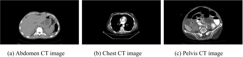
The different types of CT image used in the validation set
Table 9.
Performance evaluation of AbSeg in the validation dataset
| Images | Jaccard | Dice | Sensitivity | Specificity | CA | Precision | Kind of CT Scan |
|---|---|---|---|---|---|---|---|
| Image_1 | 99.6617 | 99.8306 | 100 | 99.8193 | 99.8821 | 99.6617 | Abdomen |
| Image_2 | 99.4603 | 99.7294 | 100 | 99.7984 | 99.8530 | 99.4603 | Abdomen |
| Image_3 | 99.7768 | 99.8883 | 100 | 99.9639 | 99.9689 | 99.7768 | Abdomen |
| Image_4 | 99.6630 | 99.8312 | 99.8812 | 99.8508 | 99.8631 | 99.7813 | Pelvis |
| Image_5 | 99.4940 | 99.7464 | 99.8930 | 99.8226 | 99.8442 | 99.6001 | Chest |
| Image_6 | 99.6902 | 99.8448 | 99.6902 | 100 | 99.9374 | 100 | Abdomen |
| Image_7 | 99.5080 | 99.7534 | 99.6493 | 99.9317 | 99.8400 | 99.8578 | Chest |
| Image_8 | 99.5626 | 99.7808 | 100 | 99.8857 | 99.9093 | 99.5626 | Chest |
| Image_9 | 99.2873 | 99.6424 | 99.7758 | 99.9058 | 99.8849 | 99.5094 | Pelvis |
| Image_10 | 99.7761 | 99.8879 | 100 | 99.8537 | 99.9115 | 99.7761 | Chest |
| Image_11 | 99.6485 | 99.8239 | 99.8713 | 99.8541 | 99.8609 | 99.7766 | Chest |
| Image_12 | 99.6514 | 99.8254 | 100 | 99.8301 | 99.8857 | 99.6514 | Abdomen |
| Image_13 | 99.6115 | 99.8054 | 100 | 99.8017 | 99.8685 | 99.6115 | Abdomen |
| Image_14 | 99.5779 | 99.7885 | 99.8856 | 99.7638 | 99.8166 | 99.6916 | Chest |
| Image_15 | 99.6063 | 99.8028 | 99.8924 | 99.9045 | 99.9015 | 99.7133 | Chest |
| Image_16 | 99.4921 | 99.7454 | 99.6810 | 99.9642 | 99.9192 | 99.8099 | Abdomen |
| Image_17 | 99.3393 | 99.6685 | 99.8051 | 99.8967 | 99.8801 | 99.5324 | Abdomen |
| Image_18 | 99.5663 | 99.7827 | 100 | 99.6938 | 99.8202 | 99.5663 | Chest |
| Image_19 | 99.5410 | 99.7700 | 99.8667 | 99.8052 | 99.8281 | 99.6735 | Chest |
| Image_20 | 99.5526 | 99.7758 | 99.8819 | 99.7938 | 99.8276 | 99.6699 | Chest |
| Image_21 | 99.6389 | 99.8191 | 100 | 99.8450 | 99.8914 | 99.6389 | Abdomen |
| Image_22 | 99.4790 | 99.7388 | 100 | 99.7879 | 99.8491 | 99.4790 | Pelvis |
| Image_23 | 99.5120 | 99.7554 | 99.8534 | 99.8273 | 99.8360 | 99.6576 | Chest |
| Image_24 | 99.6653 | 99.8324 | 100 | 99.8144 | 99.8804 | 99.6653 | Abdomen |
| Image_25 | 99.4734 | 99.7360 | 100 | 99.7937 | 99.8516 | 99.4734 | Abdomen |
| Image_26 | 99.6770 | 99.8382 | 100 | 99.8031 | 99.8775 | 99.6770 | Abdomen |
| Mean | 99.5736 | 99.7863 | 99.9087 | 99.8466 | 99.8726 | 99.6644 | – |
Table 10.
Average performance of AbSeg for different types of CT images
| Kind of CT scan | Jaccard | Dice | Sensitivity | Specificity | CA | Precision |
|---|---|---|---|---|---|---|
| Abdomen (12 images) | 99.5948 | 99.7970 | 99.9314 | 99.8609 | 99.8913 | 99.6632 |
| Chest (11 images) | 99.5768 | 99.7880 | 99.8903 | 99.8306 | 99.8542 | 99.6859 |
| Pelvis (3 images) | 99.4764 | 99.7375 | 99.8857 | 99.8482 | 99.8657 | 99.5899 |
Table 11.
Performance evaluation of AbSeg for different resolutions
| Dataset | Jaccard | Dice | Sensitivity | Specificity | CA | Precision |
|---|---|---|---|---|---|---|
| Training (16 images) | 98.9463 | 99.4699 | 100 | 98.4731 | 99.3838 | 98.9816 |
| Test (16 images) | 99.3629 | 99.6798 | 99.9135 | 99.2271 | 99.6308 | 99.4489 |
| Validation (26 images) | 99.5736 | 99.7863 | 99.9087 | 99.8466 | 99.8726 | 99.6644 |
In Fig.7, the abdomen, chest, and pelvis areas change as they are diverse from one another, and the shape of the ROIs seems non-proportional. As it differs from the training and test datasets, the validation set includes high-resolution CT images. Herein, PET/CT images are not included in the validation data because the segmentation operation of these images constitutes another qualified paper because PET/CT images include the arm parts of patients, which prevent the accurate segmentation of ellipsoid ROIs.
According to Table 10, the segmentation performance of AbSeg remains remarkable for the abdomen and it can segment the abdomen better than the chest and pelvis CT images for all metrics. In future evaluation, its usage may be extended to chest and pelvis CT images in terms of including an ellipsoid ROI as in abdomen CT images, but the amount of data should be increased to generalize the performance of AbSeg to chest and pelvis CT images. Currently, it can be seen that AbSeg can segment abdominal CT images with a high success rate, and its performance seems remarkable for similar shaped ROIs and the chest and pelvis areas.
Table 11 reveals that AbSeg performs the task of abdomen segmentation on different datasets with higher performance for approximately all metrics (except sensitivity) compared to trials realized on training and test datasets. It can be concluded here that the resolution quality directly affects the system’s output, and a higher resolution is required to attain better segmentation results.
Conclusions
This study contains an efficient and statistical structure for the optimum segmentation of the abdominal region in CT images. According to the results, AbSeg performs the task of abdomen segmentation under different handicaps that occur in abdominal CT images. Besides, it obtained very high segmentation results for the above six statistical metrics, with respective rates of 98.95, 99.2, and 99.57% for the training, test, and validation sets. Moreover, it was not affected by the appearance of the bed section, patient information, narrow histogram, poor contrast, or low-quality edges by processing sequential operators that eliminate the handicaps. In addition, AbSeg is designed using optimal operators and parameters for the segmentation of the abdominal region.
Table 12 shows the literature comparison of studies based on abdomen segmentation. Herein, it should be remembered that the results of AbSeg can be obtained on the segmentation of the rectangle surrounding the abdomen part. In other words, the results are based on a rectangle ROI that surrounds the abdomen, meaning that a higher performance is achieved in the event that the rectangle overlaps the edges of the abdomen.
Table 12.
Performance evaluation of AbSeg sections
In future work, we want to use AbSeg to detect and segment different types of tumors that can occur in the abdomen. Moreover, the usage of AbSeg will be extended to segment different regions in other scan types.
Acknowledgements
This work is supported by the Coordinatorship of Selcuk University’s Scientific Research Projects.
Contributor Information
Hasan Koyuncu, Phone: + 90 332 223 37 15, Email: hasankoyuncu@selcuk.edu.tr.
Rahime Ceylan, Email: rpektatli@selcuk.edu.tr.
Mesut Sivri, Email: drmesutsivri@gmail.com.
Hasan Erdogan, Email: dr.hasanerdogan@gmail.com.
References
- 1.Koss JE, Newman FD, Johnson TK, Kirch DL. Abdominal organ segmentation using texture transforms and a hopfield neural network. IEEE T Med Imaging. 1999;18:640–648. doi: 10.1109/42.790463. [DOI] [PubMed] [Google Scholar]
- 2.Zhou Y, Bai J. Multiple abdominal organ segmentation: an atlas-based fuzzy connectedness approach. IEEE T Inf Technol B. 2007;11:348–352. doi: 10.1109/TITB.2007.892695. [DOI] [PubMed] [Google Scholar]
- 3.Wachinger C, Fritscher K, Sharp G, Golland P. Contour-Driven Atlas-Based Segmentation. IEEE T Med Imaging. 2015;34:2492–2505. doi: 10.1109/TMI.2015.2442753. [DOI] [PMC free article] [PubMed] [Google Scholar]
- 4.Xu Z, Burke RP, Lee CP, Baucom RB, Poulose BK, Abramson RG, Landman BA. Efficient multi-atlas abdominal segmentation on clinically acquired CT with SIMPLE context learning. Med Image Anal. 2015;24:18–27. doi: 10.1016/j.media.2015.05.009. [DOI] [PMC free article] [PubMed] [Google Scholar]
- 5.Dennis LSE: Automated Segmentation of Soft tissue in Abdominal CT scans. Dissertation, National University of Singapore, 2009
- 6.Rangayyan RM, Banik S, Boag GS. Landmarking and segmentation of computed tomographic images of pediatric patients with neuroblastoma. Int J Comput Ass Rad. 2009;4:245–262. doi: 10.1007/s11548-009-0289-y. [DOI] [PubMed] [Google Scholar]
- 7.Xu Z, Conrad BN, Baucom RB, Smith SA, Poulose BK, Landman BA. Abdomen and spinal cord segmentation with augmented active shape models. J Med Imag. 2016;3:036002. doi: 10.1117/1.JMI.3.3.036002. [DOI] [PMC free article] [PubMed] [Google Scholar]
- 8.Gonzalez RC, Woods RE, Eddins SL. Digital image processing using MATLAB. New York: McGraw Hill Education; 2009. [Google Scholar]
- 9.Lim JS: Two-Dimensional Signal and Image Processing, Englewood Cliffs: Prentice-Hall, 1990
- 10.Korn GA, Korn TM: Mathematical handbook for scientists and engineers: Definitions, theorems, and formulas for reference and review. Mineola: Courier Corporation, 2000
- 11.Zuiderveld K: Contrast limited adaptive histogram equalization. In: Heckbert PS (Ed.), Graphics gems IV. San Diego: Academic Press Professional Inc., 1994, pp 474–485
- 12.Chuang KS, Tzeng HL, Chen S, Wu J, Chen TJ. Fuzzy c-means clustering with spatial information for image segmentation. Comput Med Imag Grap. 2006;30:9–15. doi: 10.1016/j.compmedimag.2005.10.001. [DOI] [PubMed] [Google Scholar]
- 13.Yang Y, Huang S. Image Segmentation by Fuzzy C-Means Clustering Algorithm with A Novel Penalty Term. Comput Inform. 2007;26:17–31. [Google Scholar]
- 14.Clark K, Vendt B, Smith K, Freymann J, Kirby J, Koppel P, Moore S, Phillips S, Maffitt D, Pringle M, Tarbox L, Prior F. The Cancer Imaging Archive (TCIA): Maintaining and Operating a Public Information Repository. J Digit Imaging. 2013;26:1045–1057. doi: 10.1007/s10278-013-9622-7. [DOI] [PMC free article] [PubMed] [Google Scholar]
- 15.Albertina B, Watson M, Holback C, Jarosz R, Kirk S, Lee Y, Lemmerman J: Radiology data from the cancer Genome Atlas Lung Adenocarcinoma [TCGA-LUAD] collection. Cancer Imaging Arch, 2016. 10.7937/K9/TCIA.2016.JGNIHEP5
- 16.Labatut V, Cherifi H: Accuracy measures for the comparison of classifiers. arXiv: 1207.3790, 2012
- 17.Franklin SW, Rajan SE. Computerized screening of diabetic retinopathy employing blood vessel segmentation in retinal images. Biocybern Biomed Eng. 2014;34:117–124. doi: 10.1016/j.bbe.2014.01.004. [DOI] [Google Scholar]
- 18.Sethi G, Saini BS. Computer aided diagnosis system for abdomen diseases in computed tomography images. Biocybern Biomed Eng. 2016;36:42–55. doi: 10.1016/j.bbe.2015.10.008. [DOI] [Google Scholar]
- 19.Alivar A, Danyali H, Helfroush MS. Hierarchical classification of normal, fatty and heterogeneous liver diseases from ultrasound images using serial and parallel feature fusion. Biocybern Biomed Eng. 2016;36:697–707. doi: 10.1016/j.bbe.2016.07.003. [DOI] [Google Scholar]
- 20.Lee H, Troschel FM, Tajmir S, Fuchs G, Mario J, Fintelmann FJ, Do S: Pixel-Level Deep Segmentation: Artificial Intelligence Quantifies Muscle on Computed Tomography for Body Morphometric Analysis. J Digit Imaging, 2017, pp 1–12 [DOI] [PMC free article] [PubMed]
- 21.Koyuncu H, Ceylan R: A hybrid tool on denoising and enhancement of abdominal CT images before organ & tumour segmentation. In: 37th IEEE International Conference on Electronics and Nanotechnology (ELNANO 2017). Kiev: IEEE, 2017, pp 249–254. 10.1109/ELNANO.2017.7939757
- 22.Koyuncu H, Ceylan R: Elimination of White Gaussian Noise in Arterial Phase CT Images to Bring Adrenal Tumours into the Forefront. Comput Med Imaging Graph, 2017 [DOI] [PubMed]
- 23.Koyuncu H, Ceylan R: Optic disc segmentation with Kapur-ScPSO based cascade multithresholding. In: International Conference on Bioinformatics and Biomedical Engineering. Cham: Springer, 2016, pp 206–215. 10.1007/978-3-319-31744-1_19
- 24.Otsu N. Thresholds selection method form grey-level histograms. IEEE T Syst Man Cyb. 1979;9:62–66. doi: 10.1109/TSMC.1979.4310076. [DOI] [Google Scholar]