Case-only approach to identifying markers predicting treatment effects on the relative risk scale

Summary

Retrospectively measuring markers on stored baseline samples from participants in a randomized controlled trial (RCT) may provide high quality evidence as to the value of the markers for treatment selection. Originally developed for approximating gene-environment interactions in the odds ratio scale, the case-only method has recently been advocated for assessing gene-treatment interactions on rare disease endpoints in randomized clinical trials. In this paper, the case-only approach is shown to provide a consistent and efficient estimator of marker by treatment interactions and marker-specific treatment effects on the relative risk scale. The prohibitive rare-disease assumption is no longer needed, broadening the utility of the case-only approach. The case-only method is resource-efficient as markers only need to be measured in cases only. It eliminates the need to model the marker’s main effect, and can be used with any parametric or nonparametric learning method. The utility of this approach is illustrated by an application to genetic data in the Women’s Health Initiative (WHI) hormone therapy trial.

1. Introduction

A high priority in many clinical contexts today is the discovery of biomarkers that predict the efficacy of a treatment. Such biomarkers, called predictive, prescriptive, or treatment selection biomarkers, may be used to guide treatment selection for individual patients, with potential to reduce treatment-associated toxicities, spare the cost of ineffective treatments, and allow individuals unlikely to benefit from a treatment to pursue alternatives. Examples of established treatment selection biomarkers include the Oncotype DX recurrence score, used to guide the use of adjuvant chemotherapy for the treatment of estrogen-receptor-positive breast cancer (Paik et al., 2004, 2006), and RAS mutations which are used to guide the choice of antiepidermal growth factor receptor (EGFR) monoclonal antibodies for the treatment of colorectal cancer (Karapetis et al., 2008; Allegra et al., 2009; Douillard et al., 2013).

Retrospectively measuring markers on stored baseline samples from participants in a randomized controlled trial (RCT) and determining their associations with treatment efficacy is generally accepted as a means of providing high quality evidence as to the value of the markers for treatment selection (see, e.g. Sargent et al. (2005); Lynnn Henry and Hayes (2006); Mandrekar and Sargent (2009); Simon et al. (2009)). Outcome-dependent sampling, such as case-control sampling, may be used to increase resource-efficiency when biomarkers are expensive to measure, or specimens are difficult to obtain. There is a growing literature on statistical analysis methods for analyzing data from such retrospective marker studies (Song and Pepe, 2004; Bonetti and Gelber, 2004; Gunter et al., 2011; Foster et al., 2011; Zhao et al., 2012; Zhang et al., 2012; Huang et al., 2012; Royston and Sauerbrei, 2004; Matsouaka et al., 2014; Kang et al., 2014; Janes et al., 2014). The necessary, but not sufficient, condition for a marker to have value for treatment selection is that it should modify the treatment effect, i.e. have an interaction with the treatment.

Interaction is a fundamental concept in statistics. A statistical interaction is defined as a departure from additivity, when considering the association between two or more predictors and an outcome on some scale(Cox, 1984; De Gonzalez and Cox, 2007; Satagopan and Elston, 2013). Two potential issues arise in the pursuit of markers that have statistical interactions with treatment. First, a statistical interaction is scale-dependent: an interaction on the multiplicative odds ratio or risk ratio (or relative risk) scale may not exist, or may differ in magnitude, if examined on the risk difference scale. Second, estimating a statistical interaction on any scale depends on adequate modeling of the respective main effects. It is well established that there is hierarchy between main effects and an interaction: an interaction enters the model only if relevant main effects are also included in the model(Cox, 1984; Bien et al., 2013), and mis-specification of main effects or omission of confounding variables may introduce bias in the estimated interaction (VanderWeele et al., 2012). Consequently, interaction modeling is particularly challenging when markers are high-dimensional, and when some markers are continuous.

In observational studies, gene-environment interactions have been of substantial interest in recent years(Hutter et al., 2013). The case-only method is widely known to provide an efficient approximation of a gene-environment interaction on the odds ratio scale, under the assumption of gene-environment independence and when the disease outcome is rare(Piegorsch et al., 1994; Umbach and Weinberg, 1997). The latter condition is necessary for the case-only estimator to approximate the interaction on the odds ratio scale, while gene-environment independence can be controversial in observational studies(Albert et al., 2001). In the RCT setting where markers are measured at baseline, marker-treatment independence is ensured by randomization, if markers are measured from baseline archived specimens. Exploiting this independence, the case-only estimator of the marker by treatment interaction on the odds ratio scale has been found to be as efficient as the full-cohort approach in trials with a rare outcome(Vittinghoff and Bauer, 2006; Dai et al., 2012). Recently, the case-only method has been used to estimate the interaction odds ratio in prevention trials such as the Women’s Health Initiative (Prentice et al., 2010) and the RV144 HIV vaccine trial (Dai et al., 2014; Li et al., 2014).

This paper considers, in an RCT, marker-specific treatment effects and marker-by-treatment interactions on the relative risk scale. Estimation of such multiplicative interactions using case-only data has been considered in observational studies(Tchetgen Tchetgen and Robins, 2010; Moerkerke et al., 2010; Vansteelandt et al., 2008). The contributions of this paper lie in elucidating the benefits of the case-only method in retrospective biomarker studies in RCT, extending such method to marker selection from a high-dimensional set and prediction of marker-specific treatment effects, and connecting case-only methodologies to the growing literature in predictive markers for treatment selection. Specifically, by focusing on the marker-specific treatment effect on the relative risk scale, the prohibitive assumption that the disease is rare, not only for the overall prevalence but also in each stratum defined by baseline markers, is eliminated. Furthermore, the case-only approach does not require modeling of marker main effects, which renders it immune to main effect mis-specification and removes the difficulty to maintain the hierarchical structure of main effects and interactions when searching among high-dimensional markers for those that modify the treatment effect. Thus case-only methods can be applied to existing machine learning methods such as Lasso or regression trees. Finally, the proportion of subjects with treatment effects opposite in sign from the overall treatment effect, a key parameter in evaluating a marker’s utility for treatment selection, can be estimated by case-only methods and tested using a simple permutation test. How to perform such a test in the context of a full model with marker main effects and interactions is an open problem.

The structure of this paper is as follows. In Section 2 we describe the rationale and methodology for the case-only approach. Section 3 demonstrates in low- and high-dimensional marker settings the performance of the approach in simulations. Section 4 implements the case-only Lasso approach to discover SNPs that predict the effect of estrogen plus progestin on breast cancer risk in post-menopausal women from the Women’s Health Initiative clinical trial. We conclude with a discussion of our findings and of future research topics.

2. Methods

Consider an RCT where participants are randomized with probability π to an experimental intervention generically called “treatment” (Z = 1), or to the standard of care (Z = 0), which might be a standard treatment or no intervention at all. We assume that the clinical outcome of interest is binary; D = 1 indicates that an event occurred over a specified time frame, for example cancer recurrence within 1 year of treatment, and D = 0 indicates the absence of the event. Participants with the event are called cases and those without the event are called controls. Suppose baseline specimens (e.g. serum or tumor tissue) have been stored for all participants for a retrospective marker study. Let M be a vector of J markers measured on the stored specimens. M may be univariate, for example an existing marker signature, or high-dimensional as in the case of tumor gene expression profiling.

Let P(D = 1|Z,M) denote the risk of the event given Z and M. Define the additive marker-specific treatment effect to be Δ(M) ≡ P(D = 1|Z = 0,M) − P(D = 1|Z = 1,M). If the goal is to select between the two treatments for every individual, the event rate in the population is minimized by a rule that recommends treatment if Δ(M) > 0, and standard of care otherwise (see e.g. Song and Pepe (2004); Gunter et al. (2011); Zhang et al. (2012); Zhao et al. (2012); Janes et al. (2014)); this is called the optimal treatment rule. If, and only if, markers interact with the treatment qualitatively so that they predict positive treatment effects for some subgroups and negative for others, such rule yields a lower event rate than that achieved under the same treatment for everyone.

For low or high–dimensional M, a common approach to identifying useful markers is to use a generalized linear regression model to examine the marker-by-treatment interaction and marker-specific treatment effect,

$$g\{P(D=1\mid Z,M)\}={\beta }_0+{\beta }_1{\mathcal{W}}_0(M)+{\beta }_{2}Z+{\beta }_3{\mathcal{W}}_1(M)\ast Z.$$ (1)

Here g is a link function, commonly the logistic function, 𝒲₀(·) is the functional form of M that corresponds to the vector of marker main effects, and 𝒲₁(·) is the functional form of M that corresponds to the vector of interactions with Z. The hierarchical constraint of main effects and interactions requires that 𝒲₁ is a subset of 𝒲₀. A test of H₀ : β₃ = 0 is used to detect a marker-by-treatment interaction.

Measuring the marker on all RCT participants can be expensive, particularly if the RCT is large in size and/or the dimension of M is large. We describe an approach that requires measuring the marker in the cases only, and yet enables estimation of the marker-specific treatment effect on the relative risk scale. Let R(M) ≡ P(D = 1|Z = 1,M)/P(D = 1|Z = 0,M) denote the treatment effect relative risk given marker M. Crucially, in an RCT R(M) has the advantage of being estimable using the case data only, based on the following derivation:

$$\begin{gathered} R(M)\equiv \frac{P(D=1\mid Z=1,M)}{P(D=1\mid Z=0,M)} \\ =\frac{P(Z=1\mid M,D=1)}{P(Z=0\mid M,D=1)}·\frac{P(Z=0\mid M)}{P(Z=1\mid M)} \\ =\frac{P(Z=1\mid M,D=1)}{P(Z=0\mid M,D=1)}·\frac{1-\pi }{\pi }. \end{gathered}$$ (2)

This follows from Bayes rule and the independence between Z and M dictated by randomization. Therefore, an estimate of $\frac{P(Z=1\mid M,D=1)}{P(Z=0\mid M,D=1)}$ that uses marker data from the cases only, together with the design constant π, provides an estimate of R(M). Note that I (Δ(M) > 0) = I (R(M) < 1). Thus, evaluating the treatment effect on the relative risk scale will not cause us to overlook the existence of markers that have qualitative interactions with the treatment, and treatment rules developed on the relative risk scale are identical to those on the absolute risk scale.

Writing (2) as the logarithm of the odds of treatment among cases, we have

$$log\left\{\frac{P(Z=1\mid M,D=1)}{P(Z=0\mid M,D=1)}\right\}=log\left\{\frac{\pi }{1-\pi }\right\}+log\left\{\frac{P(D=1\mid Z=1,M)}{P(D=1\mid Z=0,M)}\right\}.$$

If we postulate an exponential marker-specific treatment effect model,

$$R(M)\equiv \frac{P(D=1\mid Z=1,M)}{P(D=1\mid Z=0,M)}=exp\{{\beta }_2+{\beta }_3{\mathcal{W}}_1(M)\},$$

we can estimate β₂ and β₃, the main treatment effect and the marker-by-treatment interaction on the relative risk scale, by a logistic regression model for the probability of being assigned to the active treatment among cases

$$log\left\{\frac{P(Z=1\mid M,D=1)}{P(Z=0\mid M,D=1)}\right\}=log\left\{\frac{\pi }{1-\pi }\right\}+{\beta }_2+{\beta }_3{\mathcal{W}}_1(M).$$ (3)

More generally, the case-only approach provides a valid estimate of the marker-specific treatment effect on the relative risk scale, R(M). Importantly, the data-generating mechanism need not be exponential for the parameter R(M) to be of interest, and therefore for the case-only design to apply.

Along these lines, any regression or machine learning method that produces probability estimates, such as the Lasso or adaptive Lasso, classification trees, random forests, or support vector machines, can be applied to estimate R(M). In the genetics and genomics era, one of main challenges is to select a subset of relevant markers from a high-throughput genomic profiling experiment. The primary goal is marker selection, which will lead to subsequent validation studies for estimation and characterization of treatment effects. In simulations and a data application, we will select markers using the case-only Lasso logistic regression, a representative machine learning approach, where there are J markers in M modeled additively using linear terms:

$$log\left\{\frac{P(Z=1\mid M,D=1)}{P(Z=0\mid M,D=1)}\right\}=log\left\{\frac{\pi }{1-\pi }\right\}+{\beta }_2+\sum _{j=1}^J{\beta }_{3j}{M}_j,$$

subject to Σ_j |β_3j| ≤ λ. After the shrinkage estimation, non-zero β̂_3j suggests a marker-by-treatment interaction; the estimated marker-specific treatment effect is $\widehat{R}(M)=exp({\widehat{\beta }}_2+{\sum }_{j=1}^J{\widehat{\beta }}_{3j}{M}_j)$.

Having a marker-by-treatment interaction is necessary but not sufficient for a marker to be useful for treatment selection. Given an interaction, a key question is the size of the marker-defined subgroup with a treatment effect of the opposite sign as the overall treatment effect(Gunter et al., 2011; Huang et al., 2012; Janes et al., 2014). The larger the subgroup, the more impact the marker may have. Suppose the intent-to-treat effect of the treatment reduces the disease risk. We are interested in determining whether there are marker configurations in the study population such that R(M) > 1. Put into statistical language, the null and alternative hypotheses are

$${\mathrm{H}}_0:R(M)<1,\forall M\text{vs.}{\mathrm{H}}_1:R(M)>1\text{for}\text{some}M.$$

Testing H₀ against H₁ is not trivial when markers are selected by adaptive procedures such as Lasso. Indeed, we are not aware of any testing procedure for estimation and selection methods derived from the risk model (1). However, the case-only procedure provides a straightforward permutation test: the treatment labels among cases can be permuted to generate a null distribution of P(R̂(M) > 1) after adaptive marker selection. We will assess the performance of this permutation test in our simulation study.

3. Simulations

3.1 Cost and efficiency for a single marker: proof-of-concept

We simulated 1000 datasets, each with 1000 participants having a binary treatment assignment (Z) with frequency 0.5, a binary marker M with frequency 0.3, and a binary disease outcome (D) generated using a log-linear model P(D = 1|Z,M) = exp(β₀+0.3 * M+β₁*M*Z). We varied β₀ to obtain different overall event rates in the trial population (~0.05, ~0.15, ~0.40), and we varied β₁ to examine different interaction effect sizes (0, log(1.5), log(2)). The case-only approach is compared to the case-control approach that samples all cases and an equal number of controls in estimating the relative risk interaction β₁ using the correctly-specified log-linear model. Figure 1 shows the percentage estimation efficiency of β₁ and the percentage samples used relative to the full-cohort approach, under the three event rates and the three interaction sizes. When the event rate is approximately 5%, the case-only approach yields remarkable estimation efficiency (90 ~ 95%), while requiring that only 5% of samples have markers measured. The standard 1:1 case-control approach uses twice the number of samples, yet only achieves 50 ~ 70% efficiency. As the event rate increases, the cost-efficiency advantage of the case-only approach diminishes, since the controls are more and more informative about the relative risk interaction.

Figure 1.

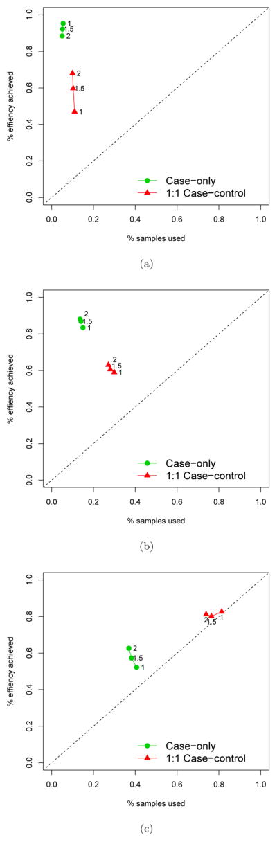
Comparison of the efficiency achieved when estimating a single marker-by-treatment interaction and the fraction of samples used in a RCT between the case-only sampling approach and the 1:1 case-control sampling approach. The full cohort sampling serves the benchmark (100%) for the efficiency and the samples used in analysis. Three scenarios were considered: (a) The overall event rate is ~5%; (b) The overall event rate is ~15%; (c) The overall event rate is ~40%.

3.2 The benefit of avoiding main effect modeling

To unbiasedly estimate interactions, main effects need to be correctly specified; otherwise, the interaction may absorb the inadequately specified main effects, leading to a biased interaction estimate. The case-only estimator eliminates the need for modeling marker main effects, and therefore is immune to main effect mis-specification. In the simulation experiments below, we generate data from two models to illustrate this advantage of the case-only approach over the standard approach. One model contains an unknown confounding factor M₂, and the other has a quadratic main effect:

$$logP(D=1\mid Z,M_1,M_2)=-1.5+{\beta }_1{M}_1-log(2)M_2+{\beta }_2{M}_1\ast Z$$ (4)

$$logP(D=1\mid Z,M)=-2+{\beta }_1{(M-1)}^2+{\beta }_{2}M\ast Z$$ (5)

In (4), the markers M₁ and M₂ are both binary with frequency 0.5, and they are correlated with odds ratio 2.25. In (5), M is distributed as 𝒩(1, 1), winsorized at 0 and 2. The treatment assignment is binomial with frequency 0.5 and independent of the marker(s). 1000 simulated datasets were created, each with 1000 participants. The comparator is the standard full log-linear interaction model, fit to the 1:1 case-control sample with inverse probability weighting.

Figure 2 shows the comparison of the absolute bias for estimating the marker-by-treatment interaction β₂, under the two models (4–5), where the size of the marker’s main effect is moderate (log(1.5)) or strong (log(2.5)). In any of the four scenarios, the case-only estimator appears to be unbiased or have little bias due to finite-sample performance, while the standard method applied to the case-control data yields considerable bias once the true interaction is not zero. Under the null hypothesis that there is no marker-by-treatment interaction, incorrect modeling of the marker’s main effect does not affect the interaction, and therefore the test of H₀ : β₂ = 0 is valid. However the bias appears as the interaction effect size increases. The bigger the main effect, the greater the bias that results from incorrect modeling of the main effect. These examples showcase the robustness of the case-only approach which does not require main effect modeling.

Figure 2.

Comparison of the absolute bias for estimating a single marker-by-treatment interaction on the log relative risk scale when the marker main effect is mis-specified between the case-only approach and the 1:1 case-control approach. Four scenarios of mis-specifications were considered: (a) Omitting a confounding variable when the main effect of the marker is moderate, log(1.5); (b) Omitting a confounding variable when the main effect of the marker is strong, log(2.5);(c) Mis-specifying the quadratic main effect of the marker by using a linear main effect and the quadratic effect is moderate, log(1.5); (d) Mis-specifying the quadratic main effect of the marker by using a linear main effect and the quadratic effect is strong, log(2.5)

3.3 Case-only approach to marker selection

The case-only approach can be directly applied to select markers that interact with treatment on the relative risk scale, without having to model the potentially high-dimensional main effects for the markers. We now investigate in simulations whether its simplicity in modeling translates to better performance for marker selection. For 2000 participants, one hundred independent binary markers were generated with frequency distributed in a uniform distribution between 0.05 and 0.45. Ten of the 100 markers predict risk and/or treatment effect, as characterized by the following log-linear model

$$P(D=1\mid Z,\mathbf{M})=exp(-2.5+\sum _{j=1}^{10}{\beta }_{1j}{M}_j+{\beta }_2\ast Z+\sum _{j=1}^{10}{\beta }_{3j}{M}_j\ast Z).$$ (6)

The case-only Lasso logistic regression is used to select markers and estimate the treatment effect on the relative risk. The comparator is the standard Lasso log-linear regression, applied to 1:1 case-control samples with 100 marker main effects, 1 treatment main effect, and 100 marker-by-treatment interactions. The case-control sampling is accounted for by inverse probability weighting. The standard Lasso approach ignores the hierarchical structure of main effects and interactions, but is as easy to implement. Ten-fold cross-validation is used to specify the Lasso penalty parameter for both approaches.

Two scenarios are presented to help explain the differential performance between the standard Lasso approach and the case-only Lasso. In the first scenario, marker effects on the risk in the control arm and marker by treatment interactions are in opposite signs, so that marginally the marker effect is small. Specifically, β₂ = 0; β_1j = log(1.5) if j ≤ 7, β_1j = −log(1.5) if 7 < j ≤ 10; and β_3j = −log(2) if j ≤ 7, β_3j = log(2) if 7 < j ≤ 10. We show that this model set-up makes it difficult for markers to enter the model as main effects first in the standard Lasso approach. In the second scenario, marker effects on risk are present only in the treatment arm, but not in the control arm. In this scenario, markers have non-negligible marginal effects, making them easier to enter the model first in the standard Lasso approach. Specifically, β₂ = 0, β_1j = 0 for all j; β_3j = −log(2) if j ≤ 7, β_3j = log(2) if 7 < j ≤ 10. The overall event rate is ~10% for both scenarios, respectively.

In the left two panels in Figure 3, we compare the performance of the two approaches in the number of falsely selected interacting markers (among 90) and the number of correctly selected interacting markers (among 10) across 100 simulated datasets. When the marker effect in the control arm and the marker-specific treatment effect are in the opposite sign, the case-only approach markedly outperforms the standard approach, as the former yields a larger number of true positive markers selected given the same number of false positive markers. This is because the standard Lasso algorithm may miss the main marker effects in this case, which will adversely affect the selection of the interaction effect. Because the case-only approach directly models the interactions, it does not suffer this problem. In the second scenario, the marker effects are only in the treatment arm, and so the absence of a main marker effect does not influence selection of interaction. In this case the standard Lasso approach performs slightly worse than the case-only approach, mainly because of dimension reduction in the case-only approach.

Figure 3.

Comparison of marker selection performance and individual treatment effect estimation using selected markers between the case-only Lasso approach and the 1:1 case-control Lasso approach. One hundred markers were generated, ten of which modified treatment effect. Two scenarios were considered: (a) and (b) are for the scenario where the interactions are in the opposite sign relative to main marker effects. (c) and (d) are for the scenario where main marker effects are zero. (a) and (c) show the performance of marker selection when marker-by-treatment interactions are qualitative or quantitative, respectively. Correspondingly, (b) and (d) show the ability to estimate marker-specific treatment effects on the relative risk scale. The lines in (a) and (c) are loess fit regressing the number of true positives on the number of false positives.

The two panels on the right in Figure 3 show the distribution of the spearman correlation between the estimated marker-specific treatment effects (individual treatment effects) and the true marker-specific treatment effects, both on the relative risk scale, across the 100 simulations. If no markers are selected using the Lasso regression, the correlation will be zero. Corresponding to the marker selection performance, the correlations for the case-only approach are remarkably higher than the standard Lasso approach in the first scenario, and slightly higher in the second scenario. The superiority of the case-only approach comes from the fact that, by removing the influence of main-effect modeling, interactions are modeled directly and the dimension of the feature space for model selection is reduced by half.

3.4 Case-only approach to assessing treatment selection by selected markers

For markers selected by an adaptive procedure such as Lasso, it is of interest to assess whether these markers, collectively, define a subgroup that has a treatment effect opposite in sign compared to the overall intent-to-treat treatment effect. We use a permutation test to accomplish this: treatment labels are permuted among cases. The case-only estimate of the overall treatment effect will not be changed in permutated datasets, however all gene-treatment interactions are removed by permutation. We generated four scenarios for treatment main effect, marker main effects, and marker-treatment interactions, each will be additionally varied in sample size and overall disease probability by changing the intercept parameter. We let β₂ = −0.5 so that there is a negative treatment effect when no marker has an interaction. Similar to the scenarios considered in Section 3.3, in the first scenario and for the main genetic effects we let β_1j = log(1.5) if j ≤ 7, β_1j = −log(1.5) if 7 < j ≤ 10. For gene-treatment interactions, we let β_3j = −log(1.5) if j ≤ 7, β_3j = log(1.5) if 7 < j ≤ 10. In the second scenario we let all main genetic effects be zero, and set β_2j = −log(1.5) if j ≤ 7, β_2j = log(1.5) if 7 < j ≤ 10. In the third scenario, we generated main marker effects by β_1j = log(1.5) if j ≤ 7, β_1j = −log(1.5) if 7 < j ≤ 10. We generated interactions by β_3j = −log(1.5) if j ≤ 7, β_3j = log(1.5) if 7 < j ≤ 10. In these three scenarios, approximately 2.5% participants have treatment effect opposite in sign compared to the overall treatment effect. The overall treatment effect in the scale of relative risk is 0.35, 0.47, and 0.54 respectively. We also generated a null model without interactions and β_1j = log(1.5) if j ≤ 7, β_1j = −log(1.5) if 7 < j ≤ 10, β_3j = 0 for j = 1, .., 100. In all simulation models we performed the permutation test using 500 permutations. The test statistic is the proportion of participants with a positive estimated treatment effect. One thousand simulated datasets were generated for each setting, each time using 500 permutations to compute the permutation-based p-value. We varied the sample size of the RCT from 2000 to 4000.

Table 1 shows the type I error and the power of the proposed permutation test. For either of two sample sizes and two disease probabilities being examined, the empirical type I error when no marker modifies the treatment effect is very close the nominal level (0.05). When 10 out of 100 markers have interactions, the power for detecting a subgroup with a positive treatment effect increases with sample size and disease probability, but decrease from scenario 1 to scenario 3. This is because the overall treatment effect decrease from scenario 1 to 3, rendering it harder to reject the null in the permutation test, even though the proportion of participants with a positive treatment effect remains similar. Note that in most of low power scenarios, the power to detect a subgroup with positive treatment effect is higher than the power to detect any of the 10 interacting markers with a family-wise error rate of 0.05. The power advantage of the former approach is less pronounced in the higher power settings.

Table 1.

Performance of the permutation test for assessing marker-based treatment selection

Disease Probability	Sample size		Permutation test* for a subgroup effect of opposite sign	Bonferroni test for any single M × T interaction
≈0.10	N=2000	Type I error	0.044	0.026
		Power(scenario 1)	0.144	0.046
		Power(scenario 2)	0.108	0.040
		Power(scenario 3)	0.076	0.032
	N=4000	Type I error	0.050	0.028
		Power(scenario 1)	0.276	0.210
		Power(scenario 2)	0.284	0.216
		Power(scenario 3)	0.166	0.176
≈0.20	N=2000	Type I error	0.064	0.034
		Power(scenario 1)	0.250	0.124
		Power(scenario 2)	0.280	0.224
		Power(scenario 3)	0.270	0.246
	N=4000	Type I error	0.064	0.044
		Power(scenario 1)	0.464	0.468
		Power(scenario 2)	0.632	0.624
		Power(scenario 3)	0.672	0.662

^*Permutation test detects evidence that a marker-specific subgroup has a treatment effect with the opposite sign of the overall treatment effect.

4. Analysis of Women’s Health Initiative clinical trial data

The Women’s Health Initiative included a clinical trial that studied the health risks and benefits of daily oral estrogen plus progestin (E+P) therapy among postmenopausal women with no prior hysterectomy (The Women’s Health Initiative Study Group, 1998). The E+P trial was stopped early when the overall health risks including breast cancer were found to exceed the benefits (Rossouw et al., 2002; Chlebowski et al., 2003). In an intent-to-treat analysis, E+P was found to increase breast cancer risk as compared to placebo (HR=1.24, p < 0.001). However, evidence from the trial also suggested that E+P lowered the risk of some secondary outcomes such as hip fractures and diabetes (Rossouw et al., 2002; Margolis et al., 2004). There is a possibility that women may respond differently to E+P in terms of risks and benefits, depending on their inherited genetic susceptibility. It is therefore of interest to determine whether there exists a subgroup of women who do not experience increased breast cancer risk from E+P, who could be prescribed hormones for relief of post-menopausal symptoms without concern about this particular adverse effect. We examined 4988 SNPs previously studied for their associations with breast cancer incidence and intervention effects in clinical trials (Prentice et al., 2010; Huang et al., 2012). While the SNPs have been investigated using a joint model including main effects and interactions with all interventions evaluated in the WHI clinical trials, our goal in this analysis is to use the case-only Lasso logistic regression approach to determine specifically whether there are a subset of SNPs predicting heterogeneous E+P effects on breast cancer, and if so, to examine the associated marker-specific treatment effects.

There were 949 women selected for inclusion in the original case-control analysis of the SNPs. For our case-only analysis, we included data for 471 invasive breast cancer cases in this sample. The indicator of E+P or placebo was regressed on 4988 SNPs in a Lasso logistic regression model, with the offset log(π/1 − π) (π = 51%), which was fit using the R package glmnet. Missing SNP values are rare (~0.5%), and were imputed by the mean of the genotype scores (0,1, and 2) among observed values. Imputation using other methods, for example the most common genotype, did not change the markers selected. We chose the Lasso penalty parameter using 10-fold cross validation, repeated 100 times to reduce the impact of random splitting. A set of 71 SNPs was selected after we applied the selected penalty parameter to the entire dataset. Among 71 SNPs, 39 have positive estimated interactions with the treatment, and 32 have estimated negative interactions. Table 2 shows the results for the top 10 SNPs among the 71 selected, listed according to the effect size of the SNP-treatment interaction in the final model after shrinkage estimation. We listed these estimates merely to get impression of interaction effect sizes, acknowledging these shrinkage estimates can be biased toward zero. We did not provide uncertainty measures of these estimates because post-selection inference for the Lasso method using cross-validation to select the penalty parameter is currently an open problem (Taylor and Tibshirani, 2016). Notably, one of the top-ranked SNPs (rs7519783) was also reported by Huang et al. (2012).

Table 2.

List of the top 10 SNPs selected using case-only lasso logistic regression in the WHI data. Bolded SNPs were also reported by Huang et al. (2012).

Rank by effect size	SNP rs ID	Chromosome	MAF*	Marker-by-treatment interaction (relative risk scale)
1	1998646	10	0.02	1.33
2	12364102	11	0.10	1.30
3	2286036	12	0.13	1.29
4	7519783	1	0.27	1.27
5	1619521	14	0.40	1.24
6	12375908	9	0.05	0.83
7	17154583	7	0.08	1.20
8	3787757	21	0.04	0.86
9	10493234	1	0.11	0.87
10	483644	11	0.33	1.13

^*MAF = minor allele frequency

The main interest in data analysis is to investigate whether there is a subgroup, defined collectively by these selected SNPs, who did not have increased risk of breast cancer by E+P. As shown in the methods section, individual treatment effects on the relative risk scale can be predicted by the “odds of treatment” using the case-only Lasso logistic regression. We first computed these estimates for 471 cases in the case-control sample for this breast cancer analysis, using the 71 SNPs and their fitted coefficients from the Lasso regression. Notably, 29% of case women (p-value=0.003, based on 2000 case-only and treatment-label-permutated datasets as shown in Methods and simulations) were estimated to have treatment effect relative risk of less than 1, meaning that breast cancer risk is estimated to be reduced under E+P in 29% of case women, despite the overall treatment effect is hazardous. In case-control samples, cases are highly selective and do not represent the trial population. To obtain the distribution of individualized treatment effects in the entire E+P trial population, each estimated individual treatment effect in the case-control was weighted by the inverse of the sampling probabilities. A histogram of the distribution of the weighted estimated treatment effects is shown in Figure 4. About 33% of women in the E+P trial is estimated to have lower risk of breast cancer if they receive E+P. Although we did not have an independent validation dataset, these results provide preliminary evidence that there is a subgroup of women whose breast cancer risk may not be increased risk by E+P, and the selected SNPs can be used to identify this subgroup. This result should be interpreted as exploratory in nature, and the SNPs identified warrant validation in follow-up studies.

Figure 4.

Distribution of estimated individual marker-specific treatment effects using selected 71 SNPs by the case-only Lasso approach on the relative risk scale in the E+P trial. The vertical line indicates the relative risk 1. About 33% of women (those with estimated treatment effects to the left of the vertical line) are predicted to have lower breast cancer risk under E+P.

As a comparison, we have analyzed the WHI data using the case-control Lasso and the same 10-fold CV procedure to choose the penalty parameter. No marker was selected by case-control Lasso as having a gene-treatment interaction. This result highlights the benefit of the case-only approach, which reduces the feature space by half.

5. Discussion

This paper describes a resource-efficient approach to identifying biomarkers that interact with treatment on the relative risk scale in RCT. Rather than measuring the marker on all study participants, or using retrospective case-control sampling to select subjects for marker measurement, the marker is measured only on the cases–which may yield considerable specimen and cost savings. We show that the case-only data can be used to estimate the “odds of treatment” among the cases, which is equivalent to the treatment effect on the relative risk scale in a randomized trial context. Any machine learning method that produces probability estimates, such as random forests, boosting, or support vector machines, can be employed. Our simulations demonstrate that the case-only approach can, in some settings, more reliably identify markers interacting with treatment than does the standard case-control approach. Furthermore, the case-only approach can be used to test for presence of a marker-defined subgroup with a treatment effect opposite in sign from the overall treatment effect.

The proposed case-only approach is perhaps best used in early-stage, retrospective profiling experiments for selecting markers with preliminary evidence of interaction. The case-only approach also applies to other endpoints. For example long-term survivors and patients with certain adverse effects in a trial can be studied as “cases” and, if germline genetics are of interest for predicting the effect of treatment on survivorship, blood samples can be collected and assayed post-treatment since germline genetics rarely change with time. Estimating the marker-specific treatment effect on the absolute risk scale and evaluating markers for use in treatment selection would require samples from controls in addition to cases.

For most clinical applications, a qualitative marker-by-treatment interaction is desired: the marker is useful if it identifies subgroups with treatment effects opposite in sign from the overall treatment effect. However, there are clinical applications where a quantitative–but not qualitative–marker-by-treatment interaction may be sufficient for a marker to be useful for treatment selection. In particular, if the treatment has downsides such as toxicity or cost, it is compelling to consider treating only subjects with sufficiently large treatment effects (Vickers et al., 2007; Janes et al., 2013). A marker that has a quantitative interaction with treatment–so that different marker values predict treatment effects of different magnitude–may be useful, even if no marker values are associated with negative treatment effects. In such settings, the magnitude of the marker-by-treatment interaction will depend on its scale.

A limitation of the case-only approach is its requirement that the endpoint of RCT has to be binary, for example tumor response or survival at a certain time after treatment. This precludes applying it to trials with failure time endpoints such as progression-free survival and overall survival. Approximation along the lines of the rare-disease assumption is needed for case-only estimators of treatment effect to be interpreted as hazard ratios(Vittinghoff and Bauer, 2006; Dai et al., 2012).

References

- Albert PS, Ratnasinghe D, Tangrea J, Wacholder S. Limitations of the case-only design for identifying gene-environment interactions. American Journal of Epidemiology. 2001;154:587–693. doi: 10.1093/aje/154.8.687. [DOI] [PubMed] [Google Scholar]
- Allegra C, Jessup JM, Somerfield MR, et al. American Society of Clinical Oncology provisional clinical opinion: testing for KRAS gene mutations in patients with metastatic colorectal carcinoma to predict response to antiepidermal growth factor receptor monoclonal antibody therapy. Journal of Clinical Oncology. 2009;17:2091–2096. doi: 10.1200/JCO.2009.21.9170. [DOI] [PubMed] [Google Scholar]
- Bien J, Taylor J, Tibshirani R. A lasso for hierarchical interaction. The Annals of Statistics. 2013;41:1111–1141. doi: 10.1214/13-AOS1096. [DOI] [PMC free article] [PubMed] [Google Scholar]
- Bonetti M, Gelber RD. Patterns of treatment effects in subsets of patients in clinical trials. Biostatistics. 2004;5:465–481. doi: 10.1093/biostatistics/5.3.465. [DOI] [PubMed] [Google Scholar]
- Chlebowski RT, Hendrix SL, Langer RD, et al. Influence of estrogen plus progestin on breast cancer and mammography in healthy postmenopausal women: the women’s health initiative randomized trial. JAMA. 2003;289:3243–3253. doi: 10.1001/jama.289.24.3243. [DOI] [PubMed] [Google Scholar]
- Cox DR. Interaction. Internat Statist Rev. 1984;52:1–31. [Google Scholar]
- Dai JY, Kooperberg C, LeBlanc M, Prentice RL. Two-stage testing procedures with independent filtering for genome-wide gene-environment interaction. Biometrika. 2012;99:929–944. doi: 10.1093/biomet/ass044. [DOI] [PMC free article] [PubMed] [Google Scholar]
- Dai JY, Li SS, Gilbert PB. Case-only methods for competing risks models with application to assessing differential vaccine efficacy by viral and host genetics. Biostatistics. 2014;15(1):196–203. doi: 10.1093/biostatistics/kxt018. [DOI] [PMC free article] [PubMed] [Google Scholar]
- De Gonzalez AB, Cox DR. Interpretation of interaction: a review. The Annals of Applied Statistics. 2007;1:371–385. [Google Scholar]
- Douillard JY, Oliner KS, Siena S, et al. Panitumumab-FOLFOX4 treatment and RAS mutations in colorectal cancer. New England Journal of Medicine. 2013;369:1023–1034. doi: 10.1056/NEJMoa1305275. [DOI] [PubMed] [Google Scholar]
- Foster JC, Taylor JMG, Ruberg SJ. Subgroup identification from randomized clinical trial data. Statistics in Medicine. 2011;30:2867–2880. doi: 10.1002/sim.4322. [DOI] [PMC free article] [PubMed] [Google Scholar]
- Gunter L, Zhu J, Murphy S. Variable selection for qualitative interactions in personalized medicine while controlling the family-wise error rate. Journal of Biopharmaceutical Statistics. 2011;21:1063–1078. doi: 10.1080/10543406.2011.608052. [DOI] [PMC free article] [PubMed] [Google Scholar]
- Huang Y, Ballinger DG, Dai JY, Peters U, Hinds DA, Cox DR, Beilarz E, Chlebowski RT, Rossouw JE, McTienan A, Rohan T, Prentice RL. Genetic variants in the MRPS30 region and postmenopausal breast cancer risk. Genome Medicine. 2012;4:19. doi: 10.1186/gm318. [DOI] [PMC free article] [PubMed] [Google Scholar]
- Huang Y, Gilbert PB, Janes H. Assessing treatment-selection markers using a potential outcomes framework. Biometrics. 2012;68:687–696. doi: 10.1111/j.1541-0420.2011.01722.x. [DOI] [PMC free article] [PubMed] [Google Scholar]
- Hutter CM, Mechanic LE, Chatterjee N, Kraft P, Gillanders EM on behalf of the NCI Gene-Environment Think Tank. Gene-environment interactions in cancer epidemiology: a National Cancer Institue think tank report. Genetic epidemiology. 2013;37:643–657. doi: 10.1002/gepi.21756. [DOI] [PMC free article] [PubMed] [Google Scholar]
- Janes H, Brown MD, Pepe MS, Huang Y. An approach to evaluating and comparing biomarkers for patient treatment selection. International Journal of Biostatistics. 2014;10:99–121. doi: 10.1515/ijb-2012-0052. [DOI] [PMC free article] [PubMed] [Google Scholar]
- Janes H, Pepe MS, Huang Y. A framework for evaluating markers used to select patient treatment. Medical Decision Making. 2013;34:159–67. doi: 10.1177/0272989X13493147. [DOI] [PMC free article] [PubMed] [Google Scholar]
- Kang C, Janes H, Huang Y. Combining biomarkers to optimize patient treatment recommendations. Biometrics. 2014;70:695–720. doi: 10.1111/biom.12191. [DOI] [PMC free article] [PubMed] [Google Scholar]
- Karapetis C, Khambata-Ford S, Jonker D, et al. K-ras mutations and benefit from cetuximab in advanced colorectal cancer. New England Journal of Medicine. 2008;359:1757–1765. doi: 10.1056/NEJMoa0804385. [DOI] [PubMed] [Google Scholar]
- Li SS, Gilbert PB, Tomaras GD, Kijak G, Ferrari G, Thomas R, Pyo C, et al. Fcgr2c polyporphisms associate with hiv-1 vaccine protection in rv144 trial. Cancer Epidemiol Biomarkers Prev. 2014;124(9):3879–3890. doi: 10.1172/JCI75539. [DOI] [PMC free article] [PubMed] [Google Scholar]
- Lynnn Henry N, Hayes DF. Uses and abuses of tumor markers in the diagnosis, monitoring, and treatment of primary and metastatic breast cancer. The Oncologist. 2006;11:541–552. doi: 10.1634/theoncologist.11-6-541. [DOI] [PubMed] [Google Scholar]
- Mandrekar S, Sargent D. Clinical trial designs for predictive biomarker validation: One size does not fit all. Journal of Biopharmaceutical Statistics. 2009;19:530–542. doi: 10.1080/10543400902802458. [DOI] [PMC free article] [PubMed] [Google Scholar]
- Margolis KL, Bonds DE, Rodabough RL, et al. Effect of estrogen plus progestin on the incidence of diabetes in postmenopausal women: results from the women’s health initiative hormone trial. Diabetologia. 2004;47:1175–87. doi: 10.1007/s00125-004-1448-x. [DOI] [PubMed] [Google Scholar]
- Matsouaka RA, Li J, Cai T. Evaluating marker-guided treatment selection strategies. Biometrics. 2014;70:489–499. doi: 10.1111/biom.12179. [DOI] [PMC free article] [PubMed] [Google Scholar]
- Moerkerke B, Vansteelandt S, Lange C. A doubly robust test for gene-enviroment interaction in family-based studies of affected offsprings. Biostatistics. 2010;11:213–225. doi: 10.1093/biostatistics/kxp061. [DOI] [PMC free article] [PubMed] [Google Scholar]
- Paik S, Shak G, Tang G, et al. A multigene assay to predict recurrence of tamoxifentreated, node-negative breast cancer. N Engl J Med. 2004;351:2817–2826. doi: 10.1056/NEJMoa041588. [DOI] [PubMed] [Google Scholar]
- Paik S, Tang G, Shak S, et al. Gene expression and benefit of chemotherapy in women with node-negative, estrogen receptor-positive breast cancer. J Clin Oncol. 2006;24(23):3726–34. doi: 10.1200/JCO.2005.04.7985. [DOI] [PubMed] [Google Scholar]
- Piegorsch WW, Weinberg CR, Taylor JA. Non-hierarchical logistic models and case-only designs for assessing susceptibility in population based case-control studies. Statistics in Medicine. 1994;13:153–162. doi: 10.1002/sim.4780130206. [DOI] [PubMed] [Google Scholar]
- Prentice RL, Huang Y, Hinds DA, Peters U, Cox DR, Beilharz E, Chlebowski RT, et al. Variation in the fgfr2 gene and the effect of a low-fat dietary pattern on invasive breast cancer. Cancer Epidemiol Biomarkers Prev. 2010;19(1):74–9. doi: 10.1158/1055-9965.EPI-09-0663. [DOI] [PMC free article] [PubMed] [Google Scholar]
- Rossouw JE, Anderson GL, Prentice RL, et al. Risks and benefits of estrogen plus progestin in healthy postmenopausal women: principal results from the women’s health initiative randomized controlled trial. JAMA. 2002;288:321–333. doi: 10.1001/jama.288.3.321. [DOI] [PubMed] [Google Scholar]
- Royston P, Sauerbrei W. A new approach to modelling interactions between treatment and continuous covariates in clinical trials by using fractional polynomials. Statistics in Medicine. 2004;23:2509–2525. doi: 10.1002/sim.1815. [DOI] [PubMed] [Google Scholar]
- Sargent D, Conley B, Allegra C, Collette L. Clinical trial designs for predictive marker validation in cancer treatment trials. Journal of Clinical Oncology. 2005;23:2020–2027. doi: 10.1200/JCO.2005.01.112. [DOI] [PubMed] [Google Scholar]
- Satagopan JM, Elston RC. Evaluation of removable statistical interaction for binary traits. Statistics in Medicine. 2013;32:1164–1190. doi: 10.1002/sim.5628. [DOI] [PMC free article] [PubMed] [Google Scholar]
- Simon RM, Paik S, Hayes DF. Use of archived specimens in evaluation of prognostic and predictive biomarkers. J Natl Cancer Inst. 2009;101:1446–52. doi: 10.1093/jnci/djp335. [DOI] [PMC free article] [PubMed] [Google Scholar]
- Song X, Pepe MS. Evaluating markers for selecting a patient’s treatment. Biometrics. 2004;60:874–883. doi: 10.1111/j.0006-341X.2004.00242.x. [DOI] [PubMed] [Google Scholar]
- Taylor J, Tibshirani R. Post-selection inference for l-1 penalized likelihood models. 2016 doi: 10.1002/cjs.11313. arXiv:1602.07358v3. [DOI] [PMC free article] [PubMed] [Google Scholar]
- Tchetgen Tchetgen EJ, Robins J. The semiparametric case-only estimator. Biometrics. 2010;66:1138–1144. doi: 10.1111/j.1541-0420.2010.01401.x. [DOI] [PMC free article] [PubMed] [Google Scholar]
- The Women’s Health Initiative Study Group. Design of the women’s health initiative clinical trial and observational study. Control Clin Trials. 1998;19:61–109. doi: 10.1016/s0197-2456(97)00078-0. [DOI] [PubMed] [Google Scholar]
- Umbach DM, Weinberg CR. Designing and analyzing case-control studies to exploit independence of genotype and exposure. Statist Med. 1997;16:1731–1743. doi: 10.1002/(sici)1097-0258(19970815)16:15<1731::aid-sim595>3.0.co;2-s. [DOI] [PubMed] [Google Scholar]
- VanderWeele TJ, Mukherjee B, Chen J. Sensitivity analysis for interactions under unmeasured confounding. Statistics in Medicine. 2012;31:2552–2564. doi: 10.1002/sim.4354. [DOI] [PMC free article] [PubMed] [Google Scholar]
- Vansteelandt S, Vanderweele TJ, Robins JM. Multiply robust inference for statistical interactions. Journal of American Statistical Association. 2008;103:1693–1704. doi: 10.1198/016214508000001084. [DOI] [PMC free article] [PubMed] [Google Scholar]
- Vickers AJ, Kattan MW, Sargent D. Method for evaluating prediction models that apply the results of randomized trials to individual patients. Trials. 2007;8:14. doi: 10.1186/1745-6215-8-14. [DOI] [PMC free article] [PubMed] [Google Scholar]
- Vittinghoff E, Bauer DC. Case-only analysis of treatment-covariate interactions in clinical trials. Biometrics. 2006;62:769–776. doi: 10.1111/j.1541-0420.2006.00511.x. [DOI] [PubMed] [Google Scholar]
- Zhang B, Tsiatis A, Laber E, Davidian M. A robust method for estimating optimal treatment regime. Biometrics. 2012;68:1010–1018. doi: 10.1111/j.1541-0420.2012.01763.x. [DOI] [PMC free article] [PubMed] [Google Scholar]
- Zhao Y, Zeng D, Rush AJ, Kosorok MR. Estimating individualized treeatment rules using outcome weighted learning. Journal of the American Statistical Association. 2012;107:1106–1118. doi: 10.1080/01621459.2012.695674. [DOI] [PMC free article] [PubMed] [Google Scholar]