Learning by neural reassociation

Abstract

Behavior is driven by coordinated activity across a population of neurons. Learning requires the brain to change the neural population activity produced to achieve a given behavioral goal. How does population activity reorganize during learning? We studied intracortical population activity in the primary motor cortex of rhesus macaques during short-term learning in a brain-computer interface (BCI) task. In a BCI, the mapping between neural activity and behavior is exactly known, enabling us to rigorously define hypotheses about neural reorganization during learning. We found that changes in population activity followed a suboptimal neural strategy of Reassociation: animals relied on a fixed repertoire of activity patterns and associated those patterns with different movements after learning. These results indicate that the activity patterns that a neural population can generate are even more constrained than previously thought and might explain why it is often difficult to quickly learn to a high level of proficiency.

INTRODUCTION

Studies of the neurophysiological changes during learning have largely focused on individual-neuron tuning properties^1–10 and correlations between the activities of pairs of simultaneously recorded neurons^11,12. However, neurons operate within large networks, and to fully understand learning, we may need to understand how neural activity reorganizes at the population level. Recent studies have discovered tantalizing evidence of population-level mechanisms by considering the joint activity across many neurons^13–20. Population-level studies of learning have only recently begun to emerge^21–24, and our understanding of how neural population activity reorganizes during learning is far from complete.

A major challenge to understanding the neural basis of learning is that, in many experiments, it can be difficult to determine the behavioral relevance of observed changes in neural activity. Interpreting the behavioral implications of such changes requires knowledge of the causal mapping from neural activity to behavior, which is not precisely known in most behavioral paradigms. BCIs have emerged as a powerful experimental paradigm²⁵ because the experimenter explicitly defines this causal mapping and can readily manipulate the mapping to induce learning^{7–10,22–24,26–30}. Exact knowledge of the mapping enables the experimenter to interpret the behavioural relevance of observed changes in neural activity and to characterize the set of activity patterns that would achieve any particular behavioral goal.

Using the BCI paradigm, we recently found that animals can readily learn to generate certain population activity patterns²². Consider a population activity space where each axis represents the activity of one neuron and a point represents the simultaneous activity across all recorded neurons at a given time (termed a population activity pattern). We and others have observed that population activity patterns do not occupy this space uniformly^{13,14,16,18,31}. Rather, activity patterns tend to reside within a low-dimensional subspace³¹, which we refer to as the intrinsic manifold. By changing the BCI mapping mid-experiment, we found that animals could more readily learn to produce population activity patterns within the intrinsic manifold than outside of it²². Precisely how the activity patterns reorganize within the intrinsic manifold is not yet understood and is the primary focus of this study.

There are many ways population activity could reorganize within the intrinsic manifold to drive behavioral improvements during learning, and observations of behavior alone are not sufficient to deduce the neural strategies guiding these changes. To begin, we consider three possible neural strategies of learning, which make differential, testable predictions about how population activity patterns might change during learning to improve behavior. The optimal strategy is for activity patterns to realign with the BCI mapping in a manner that maximizes behavioral performance. Perhaps surprisingly, the data are inconsistent with this hypothesis. Alternatively, in analogy to visuomotor gain adaptation^32,33, neural variability might rescale along each dimension to restore the influence that each dimension of population activity had on movements prior to the perturbation. The data are also inconsistent with this hypothesis. Rather, we found that the overall repertoire of population activity patterns is preserved during learning. Specifically, the activity patterns produced after learning when intending a particular movement are remarkably similar to patterns produced before learning when intending a potentially different movement. These findings suggest that neural populations are constrained to generate activity patterns from a fixed repertoire within the intrinsic manifold, which may ultimately dictate the amount of behavioral improvement possible during learning.

RESULTS

We recorded neural population activity from the primary motor cortex (M1) in three rhesus macaques (monkeys J, L, and N) while they performed a BCI learning task (Fig. 1a). We detailed the experiment and behavioral findings for two of the animals (monkeys J and L) in previous work²². Briefly, animals modulated their neural activity to drive cursor movements to visual targets in a 2-D center-out task. We applied factor analysis (FA)^23,34–37 to the recorded spike counts to identify the intrinsic manifold and summarize the neural population activity at each moment in terms of a set of 10-D factors, z_t. The causal relationship between neural activity at time t and 2-D cursor velocity, v_t, was defined by the BCI mapping:

$${\mathrm{v}}_t={\text{Av}}_{t-1}+{\text{Bz}}_t+\mathrm{c}$$ (1)

where A, B, and c are the parameters of the BCI mapping. In this work, behavior is defined by BCI cursor movements. We exclusively studied the factors, z_t, because they capture the largest shared co-fluctuations across the neural population, and because only aspects of the spike counts that are reflected in the factors can directly affect behavior (due to equation (1)). Henceforth we refer to these factors as population activity patterns.

Figure 1.

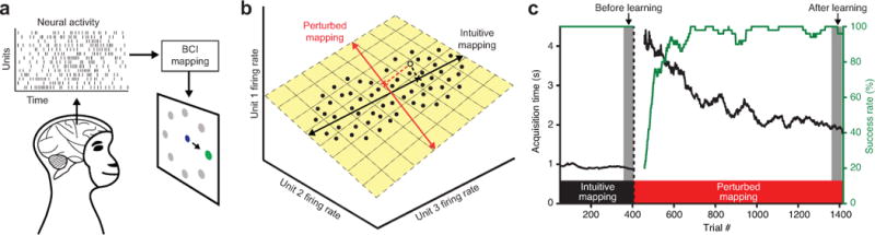
BCI learning experiment. (a) Schematic of the BCI system. The animal generates population activity patterns to drive a cursor to hit visual targets under visual feedback. (b) Population activity patterns (black dots) tend to lie in a low-dimensional subspace, termed the intrinsic manifold (yellow plane). A given activity pattern (open dot) maps to a cursor velocity (cross) according to a BCI mapping. Both the intuitive BCI mapping (black line) and the perturbed BCI mapping (red line) were designed to lie within the intrinsic manifold. (c) Behavioral performance during an example experiment (J20120525), as measured by acquisition time and success rate. Cursor velocities were initially determined by an intuitive BCI mapping (black window), and then to induce learning, the mapping was changed to a perturbed BCI mapping (red window). Left and right gray windows indicate trials analyzed “before learning” and “after learning,” respectively. Traces for acquisition time and success rate were smoothed using a causal 50-trial moving window and are not shown for the first 49 trials under each mapping.

At the beginning of each experiment, the animal proficiently controlled the cursor using an intuitive BCI mapping (Fig. 1b, black line), which was designed to be consistent with the intrinsic manifold (Fig. 1b, black line lies within yellow plane). To induce learning, we then switched to a perturbed BCI mapping (Fig. 1b, red line), which abruptly decreased the animal’s behavioral performance. Performance recovered over several hundred trials as the animal learned (Figure 1c and Supplementary Figure 1). In this work, we focus exclusively on within-manifold perturbations (Fig. 1b, red line lies within yellow plane), which altered the relationship between the factors, z_t, and cursor velocity, v_t, through changes to B in equation (1) (Supplementary Figure 2). We have shown that these perturbations can be consistently learned within a single experimental session lasting 1–2 hours²². Here, we seek to understand the learning-related changes in neural population activity that underlie this behavioral improvement.

Neural strategies of learning

Using the intuitive BCI mapping, the animal generated population activity patterns that produced the intended movement (Fig. 2a), which we define to be straight from the current cursor position to the target²⁰. However, a given activity pattern typically produces different movements through the intuitive (Fig. 2a) and perturbed (Fig. 2b) mappings. Because behavior improved under the perturbed mapping (Fig. 1c and Supplementary Figure 1), there must have been changes to the set of activity patterns produced for each intended movement (termed the movement-specific cloud of activity). There are many ways these activity patterns could have reorganized to improve behavior. We begin by considering three specific neural strategies of learning, which predict qualitatively different changes to movement-specific clouds of activity, along with the accompanying changes (or lack thereof) to the set of activity patterns taken across all intended movements (termed the overall neural repertoire). Importantly, none of these hypotheses predict novel activity patterns outside of the intrinsic manifold, as we found that on the timescale of these experiments, the intrinsic manifold remains stable (Supplementary Figure 3), and animals do not readily learn to produce outside-manifold activity patterns²².

Figure 2.

Conceptual illustrations of three hypothesized neural strategies of learning. (a) In our experiments, the BCI mapped 10-D population activity patterns to 2-D cursor velocities. Here we illustrate using 2-D activity patterns and 1-D velocities. At the beginning of each experiment, cursor velocities are determined by the intuitive BCI mapping (solid black line). Patterns to the left of the dashed line move the cursor left (L), and patterns to the right move the cursor right (R). The animal demonstrates proficient control by generating green patterns when intending to move left and purple patterns when intending to move right. High-speed movements result from patterns near the outer dotted lines. (b) Before learning, the animal’s intuitive control strategy will result in larger errors through the perturbed mapping (solid red line) than through the intuitive mapping (now gray). Errors result from purple patterns above and green patterns below the dashed line. Dotted lines represent movement speeds matching those indicated by the dotted lines in a. (c) Hypothesis 1: Realignment. Each movement-specific cloud of activity shifts to maximize behavioral performance. (d) Hypothesis 2: Rescaling. This perturbation decreases the magnitude of the behavioral output due to activity along dimension 1. To restore the influence that dimension-1 activity had on movement prior to the perturbation, variability along dimension 1 scales up. Similarly, this perturbation increases the influence of dimension-2 activity, and variability along dimension 2 scales down to compensate. (e) Hypothesis 3: Reassociation. The overall neural repertoire is unchanged relative to before learning (points are positioned as in b), but activity patterns are associated with different movement intents to improve behavioral performance (purple points above dotted line in b are now green; green points below dotted line in b are now purple). Realignment (c) and Rescaling (d) predict change to the overall neural repertoire, whereas Reassociation (e) does not.

Hypothesis 1: Learning by Realignment

The behaviorally optimal neural strategy is to realign the overall neural repertoire relative to the perturbed BCI mapping in the manner that maximizes behavioral performance (Fig. 2c). The key neural signature of Realignment is the emergence of novel activity patterns that produce high-speed movements through the perturbed BCI mapping (e.g., activity patterns beyond the outer dotted lines in Fig. 2c). These novel activity patterns represent a targeted expansion of the overall neural repertoire along the dimensions spanned by the perturbed BCI mapping.

Hypothesis 2: Learning by Rescaling

A major effect of the perturbations is a change in how strongly each factor (i.e., each element of z_t from equation (1)) influences movement velocity. Humans³² and monkeys³³ can learn to rescale the extent of arm movements when experiencing a change in the influence that their movements have on visual feedback of those movements. In analogy to this behavioral phenomenon of rescaling movements along dimensions in kinematics space, we tested for Rescaling along dimensions in population activity space. Perhaps the animal learns to rescale the variance of population activity along each neural dimension to compensate for the change in that dimension’s influence on movement due to the perturbation (Fig. 2d). Under Rescaling, the animal would learn to “push harder” along neural dimensions whose influence was attenuated by the perturbation and to “push softer” along dimensions whose influence was amplified by the perturbation.

Hypothesis 3: Learning by Reassociation

Perhaps the neural population can only generate certain patterns within the intrinsic manifold (e.g., due to underlying network constraints) such that the overall neural repertoire does not change with learning. Under Reassociation, the animal flexibly reassociates existing activity patterns with different intended movements to improve behavior (Fig. 2e). This strategy limits movements to those that can be generated by a fixed neural repertoire, and as a result, some high-speed movements that were possible through the intuitive mapping (e.g., those corresponding to activity patterns beyond the outer dotted lines in Fig. 2a) might not be possible through the perturbed mapping (e.g., there are no activity patterns beyond the outer dotted lines in Fig. 2e). In this sense, Reassociation is behaviorally suboptimal.

The key distinction between these strategies is that Realignment and Rescaling predict a change to the overall neural repertoire, whereas Reassociation predicts that the overall neural repertoire is preserved throughout learning. As such, under Realignment and Rescaling, we would expect to see novel activity patterns within the intrinsic manifold after learning. By contrast, under Reassociation, we would expect that each pattern produced after learning is similar to some pattern produced before learning.

To ground these hypotheses quantitatively, we predicted the movement-specific clouds of population activity patterns that would result from learning according to each strategy. Importantly, we ensured that all predicted activity patterns respect the intrinsic manifold, physiological limitations on the firing rates of individual neural units, and realistic levels of neural variability. We formulated these predictions using convex optimization problems³⁸ whose solutions provided the population activity patterns that would produce the maximum behavioral performance attainable subject to particular constraints (see Online Methods). The constraints on Realignment were only those mentioned above. Rescaling was further constrained to rely on a rescaled neural repertoire, and Reassociation was constrained to rely only on the before-learning neural repertoire. Based on these concrete predictions, we then asked how well each hypothesis explained the empirically observed changes in population activity and behavior.

Population-level signatures of learning strategy

To build intuition about the population-level changes in neural activity during learning, we visualized the overall neural repertoire (i.e., across all movements) during the last 50 trials under the intuitive BCI mapping (referred to as before learning) and during the 50 trials once peak performance had been achieved under the perturbed BCI mapping (referred to as after learning). The population activity patterns are defined in terms of the 10-D factors, z_t, but we can only visualize two of those dimensions at a time. We chose to visualize the 2-D outputs of the BCI mappings so that each activity pattern can be readily interpreted relative to task goals. After building qualitative intuitions using 2-D visualizations, we will quantify effects in the full 10-D population activity space.

We found that the after-learning overall neural repertoire shows a nearly complete visual overlap with the before-learning repertoire, whether activity patterns are viewed through the perturbed BCI mapping (Fig. 3, center panel) or through the intuitive BCI mapping (Supplementary Fig. 4, center panel). This visual similarity is consistent with repertoire preservation, the key hallmark of learning by Reassociation. The after-learning repertoire predicted by Reassociation shows a high degree of visual overlap with the empirical before-learning repertoire, whereas Realignment and Rescaling predict systematic repertoire changes (Supplementary Fig. 5).

Figure 3.

Visualization of population activity patterns from an example experiment (N20160728). (center) Population activity patterns recorded before learning (black; from the last 50 trials under the intuitive BCI mapping) and after learning (red; from the 50 trials of peak performance under the perturbed BCI mapping), visualized as their 2-D output through the perturbed BCI mapping. Each point represents the cursor velocity (v_x, v_y) that an activity pattern (z_t from equation (1)) contributes to cursor movement according to the perturbed mapping. Note that, although both black and red points represent recorded neural activity patterns, because the intuitive BCI mapping was in place during the before learning trials, black points represent predictions about behavior under the perturbed BCI mapping before any learning has taken place. By contrast, red points represent actual closed-loop behavior after learning. Black and red outlines encapsulate 98% of before- and after-learning patterns, respectively, and represent the overall neural repertoire. (outside) After-learning activity patterns from center plotted separately for each intended movement direction. Each of these movement-specific clouds is composed of the activity patterns recorded when the cursor-to-target direction fell within 22.5° of the labeled arrow. In this velocity space, an increase in the number of points along the cursor-to-target direction implies behavioral improvement. For example, for movements to 45°, before-learning activity patterns produced near-zero velocity, on average, but after-learning patterns produced velocities in a direction close to 45°. Outlines are reproduced from center. Gray (before learning) and red (after learning) filled regions encapsulate the patterns from each movement-specific cloud that were contained within the outlines from center. Additional details are provided in Online Methods.

Separating the overall neural repertoire into its movement-specific clouds revealed changes indicative of behavioral improvements (Fig. 3, outer panels). Consistent with the visually minimal changes to the overall neural repertoire (Fig. 3, center panel and Supplementary Fig. 4, center panel), these movement-specific changes (Fig. 3, outer panels and Supplementary Fig. 4, outer panels) were predominantly characterized by dropping before-learning activity patterns from a movement-specific cloud (e.g., Fig. 3, panel at 45°) and / or incorporating patterns that were contained within the before-learning cloud for other movements (e.g., Fig. 3, panel at 225°).

To quantify the degree of similarity between the neural repertoire before and after learning, we devised a metric based on distances between activity patterns in the 10-D population activity space (Fig. 4a). First, we computed distances between each after-learning pattern and its nearest neighbors in the before-learning overall repertoire. Then we normalized these distances by the spread of the before-learning repertoire so that repertoire preservation is indicated by values near zero, values above zero imply repertoire shift or expansion, and values below zero imply repertoire contraction (Supplementary Figure 6). The empirically observed activity did not show substantial repertoire change (Fig. 4b, “data”), which is consistent with Reassociation and the intuition conveyed by Figure 3 and Supplementary Figure 4. Realignment and Rescaling predict substantial repertoire change, which was not consistent with the data.

Figure 4.

Consistent with Reassociation, the overall neural repertoire shows minimal changes during short-term learning. (a) We measured repertoire change by assessing the distances between each after-learning population activity pattern (e.g., colored points) and its nearest neighbors (indicated by colored lines) amongst the before-learning activity patterns (black points). (b) Repertoire change measured in the data and predicted by Realignment, Rescaling, and Reassociation. Distances were normalized by the spread of the before-learning activity patterns such that positive values imply a repertoire shift or expansion, and negative values imply a repertoire contraction. Values near zero are consistent with repertoire preservation. Reassociation-predicted domain change was not significantly different from that measured in the data (p = 0.55, two-sided paired Wilcoxon signed-rank test, n = 384: 48 experiments across animals × 8 movement conditions). Realignment- and Rescaling-predicted repertoire changes were significantly different from that measured in the data (p < 10⁻¹⁰). On each box, the central line indicates the median, the bottom and top edges indicate the 25th and 75th percentiles of the data, respectively, and the whiskers extend to the 5th to the 95th percentiles of the data (n = 384).

To corroborate this Reassociation-like finding of repertoire preservation, and to further contrast with the predictions of Realignment and Rescaling, we analyzed the shared variability in the overall neural repertoire (Figures 5 and 6). First, we looked for changes in population covariability along the dimensions of the BCI mappings, which measure the extent that changes in population activity would be reflected as changes in cursor velocities. Visually, the covariability of the activity along the dimensions of the perturbed BCI mapping corresponds to the spread of the activity patterns as shown in Figure 3, and the covariability along the dimensions of the intuitive BCI mapping corresponds to the spread of patterns in Supplementary Figure 4.

Figure 5.

Consistent with Reassociation, population covariability does not change along key dimensions of the intrinsic manifold. (a) Covariability of population activity along the dimensions spanned by the intuitive BCI mapping did not change significantly during learning (p = 0.19, two-sided paired Wilcoxon signed-rank test, n = 48 experiments across animals). Each data point represents one experiment. Diagonal line indicates unity. (b) Covariability along the dimensions spanned by the perturbed BCI mapping did not change significantly during learning (p = 0.069, two-sided paired Wilcoxon signed-rank test, n = 48). (c) Predicted changes in covariability due to learning. Inset highlights the region wherein lie the observed data (defined by the data points in a and b) and the predictions of Reassociation. Rescaling and Realignment predict significantly more change in covariability along the intuitive mapping (Rescaling) and along the perturbed mapping (Realignment) than was observed in the data (p < 10⁻⁸, two-sided paired Wilcoxon signed-rank test, n = 48). Reassociation-predicted change in covariability along the intuitive mapping was not significantly different than that observed in the data (p = 0.087). Along the perturbed mapping, Reassociation-predicted covariability change was significantly different from that in the data (p = 0.006), but this effect size was small relative to that for Realignment and Rescaling. Crosses indicate ±1 S.E.M. (monkey J: n = 27 experiments; monkey L: n = 11 experiments; monkey N: n = 10 experiments).

Figure 6.

Consistent with Reassociation, population covariability does not track perturbations to the BCI mapping. (a) The intuitive mapping from an example experiment (N20160728). Each 2-D column of the B matrix from equation (1) is a pushing vector (represented by a line) describing the change in cursor position due to activity along one dimension of the population (i.e., the velocity contribution due to one factor). The direction of a pushing vector represents the direction that the corresponding activity pushes the cursor, and the length represents the strength of that push, termed the pushing magnitude. Dimensions are ordered by the amount of shared variance explained during calibration (see Online Methods). (b) The perturbed BCI mapping from the same experiment as in a. The BCI mappings (and thus the pushing vectors in a–b) were chosen by the experimenter and are not a reflection of how the animal’s neural activity changed during learning. (c) Pushing magnitudes from the intuitive mapping (lengths of lines in a). (d) Pushing magnitudes from the perturbed mapping (lengths of lines in b). (e) Change in pushing magnitude (perturbed minus intuitive) for each dimension. (f) Changes in population covariability along each dimension of the intrinsic manifold as a function of each dimension’s change in pushing magnitude due to the perturbation. Each point represents changes for one dimension of the population activity. (g) Relationships between changes in population covariance and changes in pushing magnitude. Slopes (corresponding to trend lines in f) were computed independently for each experiment using linear regression. Triangles indicate slopes for the experiment in f. Tick marks above each plot indicate means across experiments. Reassociation-predicted slopes were not significantly different from those in the data (p = 0.76, two-sided paired Wilcoxon signed-rank test, n = 48 experiments across animals). Realignment- and Rescaling-predicted slopes were significantly different from those in the data (p < 10⁻⁸).

The data did not show substantial changes in the amount of covariance projected along the intuitive (Fig. 5a) or perturbed (Fig. 5b) BCI mappings, which is again consistent with learning by Reassociation (Fig. 2e and Fig. 5c, blue). By contrast, Realignment and Rescaling, which both predict repertoire change (Fig. 4b, red and yellow), make differential predictions about the structure of those changes. Realignment predicts repertoire expansion due to the addition of novel activity patterns that have large outputs through the perturbed BCI mapping relative to patterns produced before learning (Fig. 2c). This expansion is detected as an increase in covariability along the dimensions of the perturbed mapping (Fig. 5c, red). Rescaling predicts repertoire expansion due to the addition of novel activity patterns that have large outputs through the intuitive BCI mapping (Fig. 2d). This is seen as an increase in covariability along the dimensions of the intuitive mapping (Fig. 5c, yellow). The data (Fig. 5c, black) were not consistent with these predictions of Realignment or Rescaling.

Next, we searched for changes in shared variability across the 10 dimensions of the population activity space that might be related to the particular perturbation. Recall that each factor (i.e., each element in z_t from equation (1)) represents population activity fluctuations along a particular dimension of the population activity space. Each perturbation effectively changes both the direction that each factor’s activity pushes the cursor (the direction represented by each 2×1 column of B in equation (1); Fig. 6a,b) and its pushing magnitude (the norm of that column of B; Fig. 6c–e). The learning strategies we have presented make differential predictions about how each factor’s variance should change in response to the change in that factor’s pushing magnitude due to the perturbation (Fig. 6f,g).

Realignment predicts an increasing trend between changes in pushing magnitude and changes in factor variance (Fig. 6f,g, red). Under Realignment, the movement-specific clouds of activity migrate into and spread along the dimensions spanned by the perturbed mapping (Fig. 2c). As a result, variability should increase for factors that contribute more to movement under the perturbed mapping than they did under the intuitive mapping. Rescaling predicts the opposite trend (Fig. 6f,g, yellow). If a perturbation increases (or decreases) the contribution of a particular factor toward movement, variance should decrease (or increase) for that factor to restore the influence that factor had on movement prior to the perturbation (Fig. 2d).

These predictions of Realignment and Rescaling contrast with those of Reassociation. Because Reassociation predicts that the same overall repertoire of activity patterns is used before and after learning, Reassociation predicts that the variance for each factor should not change, regardless of how each factor’s pushing magnitude had changed (Fig. 6f,g, blue). The data did not show a trend between changes in pushing magnitude and changes in factor variance (Fig. 6f,g, gray), which closely matches the predictions of Reassociation.

Behavioral consequences of learning strategy

As expected, behavioral performance dropped abruptly when BCI mapping was perturbed (Fig. 1c). This performance drop is predicted by the before-learning population activity (Fig. 7: “Before learning,” “Intuitive mapping” vs “Perturbed mapping”). After learning, behavioral performance improved substantially (“Perturbed mapping,” “Before learning” vs. “After learning”). Interestingly, after-learning behavioral performance did not completely recover to intuitive levels (“Before learning, Intuitive mapping” vs. “After learning, Perturbed mapping”).

Figure 7.

Behavioral learning is consistent with Reassociation. Acquisition time is the time elapsed between movement onset and target acquisition. “Before learning” data are from the last 50 trials under the intuitive BCI mapping (see Fig. 1c). “Before learning, Intuitive mapping” assesses the empirical closed-loop behavior during these trials. “Before learning, Perturbed mapping” predicts the behavioral performance that would result under the perturbed BCI mapping if the animal did not learn (i.e., if under the perturbed BCI mapping the animal generates the same movement-specific clouds that it had generated under the intuitive BCI mapping). “After learning, Perturbed mapping” assesses the empirical closed-loop behavior under the perturbed BCI mapping after the animal had learned. The empirical behavioral learning effect is represented by the improvement from “Before learning, Perturbed mapping” to “After learning, Perturbed mapping.” “Realignment,” “Rescaling,” and “Reassociation” assess predicted after-learning activity patterns through the perturbed BCI mapping. Reassociation-predicted acquisition times were not significantly different from the data (“After learning, Perturbed mapping” vs. “Reassociation”; p = 0.46, two-sided paired Wilcoxon signed-rank test, n = 48 experiments across animals). Realignment-predicted and Rescaling-predicted acquisition times were significantly different from the data (p = 1.6 × 10⁻⁹ and p = 0.011, respectively). On each box, the central line indicates the median, the bottom and top edges indicate the 25th and 75th percentiles of the data, respectively, and the whiskers extend to the 5th to the 95th percentiles of the data (monkey J: n = 27 experiments; monkey L: n = 11 experiments; monkey N: n = 10 experiments).

Realignment, Rescaling, and Reassociation all predict behavioral improvements due to learning. However, the extents of these predicted improvements varied (Fig. 7: “Realignment,” “Rescaling,” and “Reassociation”). The behaviorally optimal Realignment predicts substantially more behavioral improvement than shown by the animals. Rescaling predicts slightly more behavioral improvement than shown by the animals. Reassociation predicts behavioral improvement closely matched to that shown by the animals, and in doing so also predicts the incomplete recovery of behavioral performance demonstrated by the animals. These behavioral results, taken together with the repertoire preservation demonstrated in Figure 4b, suggest that a fixed neural repertoire represents a fundamental constraint on the amount of behavioral improvement that is possible during short-term learning.

Variants and mixtures of learning strategies

There is a continuum of neural strategies that could subserve learning, and of these we have thus far only considered three distinct strategies. Here we consider the possibility that learning involves variants or mixtures of the strategies presented thus far. First, we consider an attenuated variant of Realignment, in which behavioral predictions are matched to empirical after-learning behavioral performance. Second, we consider Subselection, a variant of Reassociation, in which the activity patterns produced for a given movement after learning are a subset of the patterns produced for that same movement prior to learning. Finally, we consider the possibility that learning involves a combination of Reassociation and Realignment.

The first variant we explore is Partial Realignment. Our predictions have suggested that Realignment would yield substantially better behavioral performance than animals showed empirically after learning (Fig. 7). Might it be that the animals’ population activity did change in a manner akin to Realignment, but each movement-specific cloud of activity migrated only partially toward the cloud predicted by complete Realignment (Fig. 8a)? To address this possibility, we refined the Realignment predictions to match the animals’ empirical levels of behavioral performance after learning. We found that the before-learning movement-specific clouds only needed to migrate about 15% toward the complete-Realignment clouds to match these empirical levels of behavioral performance (see Supplementary Math Note).

Figure 8.

Partial Realignment and Subselection are not consistent with the data. (a) Conceptual illustration of Partial Realignment, in which the movement-specific clouds of activity transition partially from their before-learning locations to their Complete-Realignment locations in population activity space. (b) Conceptual illustration of Subselection, in which the activity patterns used to generate a particular movement after learning are a subset of the same patterns that had been used for that movement under the intuitive BCI mapping, and are still appropriate for the same movement under the perturbed BCI mapping (filled points). Patterns that do not satisfy this criterion are no longer produced (open points). Format matches that of Figure 2 (gray line: intuitive BCI mapping; solid red line: perturbed BCI mapping; dotted red lines: set of activity patterns that map to high-speed movements through the perturbed BCI mapping, matched to dotted lines in Fig. 2). (c) Percentage of movement-specific clouds showing repertoire change. Here repertoire change was assessed for each after-learning movement-specific cloud relative to the before-learning movement-specific cloud for the same movement. Repertoire change in the data was significantly different from that predicted by Partial Realignment and that predicted by Subselection (p < 10⁻¹⁰, paired two-sided sign test, n = 384: 48 experiments across animals × 8 movement conditions). Vertical lines indicate 95% confidence intervals (Bernoulli process, n = 384).

Given that the changes in population activity predicted by Partial Realignment are subtler than those predicted by complete Realignment, we might not be able to disambiguate Reassociation and Partial Realignment when considering the overall repertoire of activity patterns across movements as in Figures 4–6. However, we can clearly disambiguate these strategies by analyzing changes in the movement-specific clouds of activity. Reassociation predicts that the movement-specific clouds shift substantially more (Fig. 2e) than predicted by Partial Realignment (Fig. 8a). To quantify these changes, we measured movement-specific repertoire change using the same distance-based metric as in Fig. 4, but applied to the movement-specific clouds rather than to the overall neural repertoire. The data showed movement-specific repertoire change that was consistent with Reassociation and was substantially greater than that predicted by Partial Realignment (Fig. 8c).

The second variant we explore is Subselection³⁹ (Fig. 8b). Subselection predicts that, for a given movement after learning, the animal produces only the activity patterns from that movement’s before-learning cloud that remain appropriate for that movement under the perturbed BCI mapping (filled points in Fig. 8b). Patterns that are no longer appropriate for that movement are no longer produced (open points in Fig. 8b). Subselection is like Reassociation in that, across all movements, the animal does not produce novel patterns after learning. However, for a particular movement, Reassociation may recruit activity patterns that were associated with other movements prior to learning, whereas Subselection cannot.

In the example experiment shown in Figure 3 and Supplementary Fig. 4, the after-learning movement-specific clouds (outer panels, red) contained a substantial number of activity patterns outside the before-learning cloud for the same movement (corresponding gray regions). This finding is inconsistent with Subselection. To test for Subselection quantitatively, we again looked at movement-specific repertoire change. Subselection predicts a substantial contraction within the movement-specific clouds (Fig. 8c, light blue bars). The data (Fig. 8c, gray bars) were not consistent with this key prediction of Subselection, but rather were consistent with the movement-specific repertoire shifts predicted by Reassociation (Fig. 8c, dark blue bars). Taken together, these analyses indicate that the animals learned by co-opting existing population activity patterns (Figures 3–6) to subserve new movement intents after learning (Fig. 8), as predicted by Reassociation.

Finally, we explore the possibility that learning engages multiple learning processes simultaneously^40–43. Our analyses have revealed that Reassociation explains the population activity (Figs. 3–6) and behavioral improvements (Fig. 7) we observed during learning. This included showing that, consistent with Reassociation, the amount of population covariability along the perturbed mapping did not change substantially due to learning (Fig. 5b,c). Upon closer inspection, we found that subtle experiment-by-experiment fluctuations in this covariability metric correlated positively with levels of behavioral learning, which is consistent with Partial Realignment (Supplementary Fig. 8). Although our analyses have already ruled out the possibility that behavioral improvements are primarily due to Realignment or Partial Realignment (Figs. 3–8), this subtle effect suggests that an element of Realignment might play a minor role, alongside Reassociation, during short-term learning.

Potential influences on learning strategy

Finally, we asked whether the design of our experiments influenced the neural strategy of learning demonstrated by the animals. One possibility is that accumulated experience controlling intuitive mappings (i.e., across many experiments) might make it progressively more difficult for a neural population to change its neural repertoire, perhaps due to a consolidation of activity patterns that are most effective at driving the intuitive mapping. If this were the case, we would expect evidence of Reassociation to become progressively stronger throughout the course of these experiments, while evidence of another learning strategy (e.g., Realignment or Rescaling) becomes progressively weaker. This was not the case. Rather, the data were consistent with learning by Reassociation throughout the entire course of the experiments (Supplementary Fig. 9).

Another possibility is that the within-manifold perturbations might not apply enough pressure to change the neural repertoire. Two pieces of evidence suggest that this is not the case. First, even after learning, animals showed a substantial performance deficit relative to intuitive-level control (Fig. 7 and Supplementary Fig. 7). Thus, there is likely pressure to continue improving behavior beyond the levels of performance we observed after learning, and yet we did not observe changes to the neural repertoire (e.g., Realignment or Rescaling) that would have driven such additional behavioral improvement. Second, when there was more pressure to change the neural repertoire, we did not observe larger changes to the neural repertoire (Supplementary Fig. 10). These two pieces of evidence indicate that the finding that animals largely learned by Reassociation is not due to a lack of pressure to show activity patterns outside the neural repertoire.

DISCUSSION

In this work, we investigated the population-level changes in neural activity that drive behavioral improvements during short-term learning. We found that repertoire preservation was the guiding constraint underlying the reorganization of population activity. After learning, animals produced roughly the same set of activity patterns across all movements as were produced before learning. What had changed was the association between movement intents and activity patterns within the neural repertoire. We showed that a neural strategy of Reassociation predicts this repertoire preservation and the extent of behavioral learning demonstrated by the animals. These levels of behavioral performance are considerably suboptimal relative to those possible via a strategy of neural Realignment, which is not constrained by repertoire preservation. Taken together, these findings indicate that, on the timescale of these experiments (1–2 hours), changes in neural activity during learning are even more constrained than previously believed.

In previous work, we found that animals can readily reorganize neural activity within the intrinsic manifold but not outside of it²². However, it remained an open question specifically how neural activity changes within the intrinsic manifold to support the behavioral learning we observed. In this work, we addressed this question by considering a range of hypotheses, all of which operate exclusively within the intrinsic manifold (i.e., they do not predict outside-manifold activity patterns, nor do they predict changes to the intrinsic manifold). Thus, the changes we considered here are fundamentally different from those that might be required for learning a BCI mapping that lies outside of the intrinsic manifold.

Several previous BCI learning studies have addressed the related question of whether behavioral improvements are driven by changes that are independent across neurons or by changes that reflect shared constraints across neurons^{8–10,22,23,27,29,44}. For short-term learning (i.e., within 1–2 hours), studies have found evidence of such shared constraints within M1^8,10,22,27 and the parietal reach region⁴⁴, and have suggested that independent-neuron learning does not play a dominant role. Informed by these studies, in this work we only considered population-level learning strategies that reflect shared constraints across neurons.

An important contribution beyond these previous studies is that our investigation into these shared constraints was performed at the level of 10-D factors (z_t in equation (1)), which provide a more comprehensive characterization of the population activity than the 1-D or 2-D kinematics-based quantities previously used to describe those constraints^8,10,27,44. In addition to capturing variables that relate directly to task kinematics, the factors we identified can also capture variables that are internal to the animal and do not directly relate to task kinematics or objectives. Together, these factors more fully describe the degrees-of-freedom in the population activity that the animal can leverage to improve behavior during learning. There are many ways that these factors could reorganize during learning while respecting shared constraints across neurons (e.g., the intrinsic manifold), and analyses of behavior alone²² are not sufficient to deduce the neural strategies guiding this reorganization. Here, we rigorously defined a range of hypotheses about how these factors might reorganize during learning and presented an analysis framework that enabled us to disambiguate between these hypotheses. Because these analyses were based on 10-D factors, they have the power to identify learning-related changes that might not be apparent in one or two kinematics-based factors.

The hypotheses we considered lie along a continuum describing the flexibility of the neural repertoire, which ranges from Realignment (most flexible) to Subselection (most constrained). Realignment can flexibly change the neural repertoire to maximize behavioral performance. Subselection constrains the activity patterns for each movement to be a subset of the patterns used for that same movement before learning. Reassociation has an intermediate flexibility because it cannot change the neural repertoire, but it can change how activity patterns within the repertoire are used. That Reassociation predicts the data well and lies between the most and least flexible strategies we considered, suggests that the breadth of hypotheses we considered was adequate.

Given additional exposure to a perturbed BCI mapping, might there be further reorganization of neural activity with corresponding improvements in behavioral performance? Further behavioral improvements would require neural changes beyond those predicted by Reassociation. One such possibility is that the animal learns to decrease neural variability in a manner that improves the ability to precisely generate activity patterns that drive high-performance movements⁴⁵. Another possibility is that the animal learns to produce novel activity patterns. For the within-manifold learning tasks considered in this work, substantial behavioral improvements would be possible if novel activity patterns could be generated within the intrinsic manifold, such as those activity patterns predicted by Realignment. We did see subtle hints of Realignment (Supplementary Fig. 8), but this was not the dominant process driving behavioral improvements on the 1–2 hour timescale of our experiments (Figs. 3–7). We cannot rule out the possibility that different task demands might accelerate learning novel activity patterns. However, animals did not show more Realignment when there was more behavioral incentive to do so (Supplementary Fig. 10), and BCI mappings outside of the intrinsic manifold are not readily learned on this same 1–2 hour timescale²². Thus, Reassociation and Realignment might operate in parallel but with vastly different timescales. When learning over longer timescales, the cumulative effect of Realignment-like changes could become a substantial driver of behavioral improvement. Such a combination of learning processes would allow for an initial reduction in errors that is largely due to Reassociation (i.e., on a timescale of hours), with further error reduction driven by Realignment (i.e., on a timescale of days to weeks).

It is currently unclear what neural mechanisms underlie the Reassociation-like reorganization we found in the population activity. Sensorimotor learning requires changes to the output signals (in our case, M1 activity) generated in response to a given sensory input. Changes to M1 activity could arise from connectivity changes between M1 neurons or from changes to the inputs of M1 for a given sensory input. While we cannot definitively disambiguate these two possibilities, our finding of neural repertoire preservation seems more consistent with changes to the inputs of M1, since connectivity changes within M1 would likely lead to changes in the repertoire. The driver of these learning-related changes could be cortical or subcortical⁴⁶, and additional experiments are needed to make these distinctions.

In this work, we took a population-level approach to study BCI learning in M1, and found that a strategy of learning by neural Reassociation predicted key features in the data. The hypotheses and analysis framework presented here in the context of a BCI task can also be used to ask whether similar population-level strategies and constraints govern learning in other contexts, such as arm movements (e.g., in M1^3,6), perceptual learning (e.g., in visual cortex¹¹), rule learning (e.g., in prefrontal cortex²¹), or associative learning (e.g., in auditory cortex¹²).

ONLINE METHODS

Experimental Procedures

Experimental procedures for monkeys J and L are described in detail in ref. ²². Procedures for monkey N were nearly identical. Here we briefly summarize the procedures and highlight any differences in the procedures for monkey N. All animal procedures were approved by the Institutional Animal Care and Use Committee of the University of Pittsburgh.

Neural recordings

Three adult male rhesus macaques (Maccaca mulatta; age, monkey J: 7 years; monkey L: 8 years; monkey N: 7 years) were each chronically implanted with a 96-channel multi-electrode array targeting proximal arm area of M1. Spikes on a given channel were identified as threshold crossings and were counted in non-overlapping 45-ms bins. We refer to each channel as a neural unit, and we refer to the set of spike counts recorded simultaneously across all channels during a single 45-ms time bin as a spike count vector. We recorded from 86.5 ± 1.40 units (mean ± one standard deviation) across 27 analyzed experiments for monkey J, 88.4 ± 0.88 units across 11 analyzed experiments for monkey L, and 93.5 ± 0.81 units across 10 analyzed experiments for monkey N.

Behavioral task

Animals performed an 8-target center-out BCI task. Each trial began with a 300 ms freeze period, during which the cursor (circle, radius 18 mm) remained at the center of the workspace. A peripheral target (circle, radius 20 mm) was displayed at the beginning of this freeze period. Animals then moved the cursor by modulating their neural activity. A water reward was delivered if the target was acquired within 7.5 s following the end of the freeze period, and the next trial was initiated 200 ms after target acquisition. If the target was not acquired within 7.5 s, there was a 1.5 s timeout before the next trial was initiated. Target locations were selected from a set of 8 uniformly spaced locations around a circle (radius, monkey J: 150 mm; monkeys L and N: 125 mm). For monkeys J and L, targets were presented in a pseudorandom order to equalize the number of successful trials for each target. For monkey N, targets were presented in a random order independent of target acquisition history. Each animal’s arms were loosely restrained during the BCI task, and animals showed little to no arm movements²².

Task flow

Each experiment began with 80 calibration trials used to identify the intrinsic manifold and to define the intuitive BCI mapping. The intuitive mapping was then used during a block of intuitive trials (monkey J: 382 ± 66.7 trials; monkey L: 269 ± 52.3 trials; monkey N: 193 ± 3.68 trials). The mapping was then changed to a perturbed BCI mapping for a block of perturbed trials (monkey J: 871 ± 66.3 trials; monkey L: 360 ± 84.9 trials; monkey N: 620 ± 60.0 trials). After the perturbed trials, the intuitive BCI mapping was reinstated for a block of washout trials (not analyzed in this work).

Identifying the intrinsic manifold and extracting population activity patterns

We used factor analysis (FA)^23,34–37 to identify the intrinsic manifold and to summarize each high-dimensional spike count vector, ${\mathrm{u}}_t\in {\mathcal{R}}^q$, in terms of a low-dimensional set of factors, ${\mathrm{z}}_t\in {\mathcal{R}}^p$, where q is the number of simultaneously recorded neural units, p is the number of factors (i.e., the dimensionality of the intrinsic manifold), and p < q. All references to “population activity patterns” refer to these factors, z_t. A new FA model was fit for each experiment based on the recorded neural activity from the calibration trials. For all analyses, factors were extracted such that dimension 1 (i.e., the first element in z_t) explains the most shared covariance across the population, dimension 2 is orthogonal to dimension 1 and explains the next most shared covariance, and so on (see Supplementary Math Note).

For consistency, we used p = 10 across all experiments. We used 10 factors (or dimensions) because that was the average dimensionality identified by FA via cross-validation over monkey J and L experiments, and because when higher dimensionalities were identified, they did not offer substantially better accounts of the data relative to using 10 factors²². We found that animals’ after-learning neural activity remained consistent with these descriptions of the intrinsic manifold (Supplementary Figure 3).

Intuitive BCI mappings

BCI mappings translated the factors, z_t, into 2-D cursor velocities, v_t, using a Kalman filter ^47,48. Intuitive BCI mappings took the form

$${\mathrm{v}}_t={\text{Av}}_{t-1}+{\text{Bz}}_t+\mathrm{c}$$ (2)

where $\mathrm{A}\in {\mathcal{R}}^{2\times 2}$ temporally smooths the velocities, $\mathrm{B}\in {\mathcal{R}}^{2\times 10}$ defines the dimensions within the intrinsic manifold that directly influence cursor movements (termed the control space), and $\mathrm{c}\in {\mathcal{R}}^2$ is a constant offset.

Each experiment began with 80 trials used to calibrate an intuitive BCI mapping. Trials involved either closed-loop BCI cursor control, passive observation of center-out cursor movements, or a combination of the two (see details below). Population activity was recorded during these trials and was paired with estimates of the animal’s intended cursor velocities. We then determined the parameters of the intuitive mapping (A, B, and c from equation (2)) based on these paired data (see Supplementary Math Note).

For monkey J, two different calibration procedures were used. In early experiments, calibration consisted of closed-loop center-out trials under the previous day’s intuitive BCI mapping. Intended cursor velocity at each timestep was taken to be in the current cursor-to-target direction with a speed equal to the current cursor speed^20,49. For monkey J’s later experiments, we used an observation-based calibration procedure, which did not depend on the previous day’s mapping. This change was made to reduce the likelihood of carry-over effects on the neural population across days. During these calibration trials, we recorded neural activity as the animal passively observed automatic center-out cursor movements straight to the target at a constant speed (0.15 m/s). Here, intended cursor velocity at each timestep was taken to be the observed cursor velocity (0.15 m/s in the center-to-target direction).

For monkeys L and N we used a hybrid of these closed-loop and observation-based approaches. These calibrations began with 16 trials (2 to each target) of the observation-based procedure. For the next 8 trials, the animal controlled cursor movements using a mapping calibrated using the data from the previous 16 trials, but the cursor was restricted to move only along the center-to-target direction (velocity components perpendicular to the center-to-target direction were scaled by a factor of 0). The next 8 trials used a mapping calibrated from the previous 24 trials, and perpendicular velocity components were scaled by a factor of 0.125. We repeated this procedure for a total of 80 trials until the animal was given complete control of the cursor (perpendicular scale factor = 1). All calibrations performed within this procedure defined intended cursor velocities to be in the center-to-target direction with speeds taken from the corresponding cursor movements that were displayed to the animal.

Animals demonstrated proficient cursor control using the intuitive BCI mapping from the very first intuitive trial of each experiment, as evidenced by success rates and acquisition times (Fig. 1). Acquisition times from the last 50 intuitive trials of each experiment are described in Figure 7 (bars labeled “Before learning,” “Intuitive mapping”; median acquisition time, monkey J: 885 ms; monkey L: 974 ms; monkey N: 636 ms).

Perturbed BCI mappings

Perturbed BCI mappings altered the relationship between recorded population activity patterns and cursor movements. In this work, we studied within-manifold perturbations, which altered the relationship between the factors, z_t, and the cursor velocity, v_t. Specifically, we permuted the ordering of the factors (i.e., the elements of z_t), which is equivalent to permuting the columns of B in equation (2) while preserving the ordering of the factors. Accordingly, perturbed BCI mappings took the form

$${\mathrm{v}}_t={\text{Av}}_{t-1}+{\mathrm{B}}^{\text{pert}}{\mathrm{z}}_t+\mathrm{c}$$ (3)

where A and c are unchanged from equation (2), and B^pert contains the permuted columns of B from equation (2). Geometrically, a within-manifold perturbation corresponds to re-orienting the control space within the intrinsic manifold (Fig. 2b). With each experiment, our aim was to select a candidate perturbation that would be difficult enough that substantial learning would be required to restore proficient control, but not so difficult as to deter the animal. Our procedure for selecting such a perturbed BCI mapping is detailed in the Supplementary Math Note.

Behaviorally, these perturbations had complex effects on cursor movements, which cannot be replicated by pure visuomotor rotations or gains (Supplementary Figure 2). Before learning, the effects of a typical perturbation can be approximately summarized by a combination of per-target velocity rotations and speed scalings. Because the perturbations were implemented in 10-D, these rotations and scalings need not be consistent across movement directions and speeds (as they would be in the case of a pure visuomotor rotation or gain). Perturbations often affected movement speeds more profoundly along one movement direction than along the perpendicular direction. Angular errors (e.g., deviations between movement direction and target direction) were also often larger for some targets than for others. For some perturbations these angular errors had a consistent sign across targets, but this was not always the case.

Animal training history

Animals were initially trained to perform cursor movements that were tied to arm movements. Once an animal demonstrated understanding of the task goals (e.g., move the cursor to the target), we transitioned the animal into the BCI paradigm by loosely restraining the animal’s arms and determining cursor movements from neural activity through a BCI mapping. Prior to the experiments analyzed in this work, animals accrued experience controlling intuitive BCI mappings through this training and through other experiments not analyzed in this work (monkey J: 19.2 months; monkey L: 1.9 months; monkey N: 2.5 months).

The experiments analyzed in this work involved within-manifold perturbations of the BCI mapping. In additional experiments not analyzed in this work, the perturbed BCI mapping was outside of the intrinsic manifold. These outside-manifold perturbation experiments were interleaved with the within-manifold perturbation experiments, and the perturbation type was selected pseudorandomly each day. The experiments analyzed spanned several months (monkey J: 4.6 months; monkey L: 6.8 months; monkey N: 4.6 months). In this work, we exclusively analyzed the within-manifold perturbations because animals showed more behavioral learning in those experiments²², and our primary goal in this work was to understand the neural underpinnings of this behavioral learning.

Selecting experiments and trials for analysis

Because our goal is to characterize changes in neural activity due to learning, we focused on the experiments in which the animals showed the most behavioral learning (i.e., improvements in cursor movements). We included an experiment for analysis if we detected significant improvements in both success rate (p < 0.05, two-sided unpaired Wilcoxon rank-sum test) and acquisition time (p < 0.05, two-sided unpaired t-test) between the first 50 perturbed trials and any subsequent block of 50 perturbed trials. For monkeys J, L, and N, 27 of 28, 11 of 14, and 10 of 11 experiments met these criteria, respectively.

In experiments that met these criteria, we analyzed the last 50 successful intuitive trials (“before learning”) and the successful trials from the 50 consecutive perturbation trials that showed the best behavioral performance (“after learning”). Here, behavioral performance was measured using a composite statistic that combines normalized success rate and normalized acquisition time (“amount of learning” from ref. ²²). Failed trials interspersed within those 50 successful trials were not analyzed because it is difficult to determine whether the animal was actively engaged in the task during failed trials.

Selecting and grouping activity patterns for analysis

We composed movement-specific clouds of activity for intended movements in each of 8 uniformly spaced directions, which correspond to the 8 target directions in the center-out task. At timestep t, we defined the intended movement direction to be the nearest of these 8 directions to the straight-to-target direction from the current cursor position. We did not introduce a lag between intended movement direction and cursor position (i.e., to account for visual feedback delays) because we have previously shown that, during BCI control, animals compensate for natural visuomotor latencies such that M1 reflects the animal’s movement intent relative to the current cursor position (rather than an outdated cursor position)²⁰. To account for visuomotor latencies at the start of each trial, we excluded data for analysis from the first 135 ms (i.e., 3 time steps in the BCI system) following target onset²⁰.

An important goal in this work was to characterize learning-related changes in the overall neural repertoire. To ensure that our findings were not biased by differences in the number of activity patterns in each movement-specific cloud (e.g., due to asymmetric cursor kinematics), we matched the number of activity patterns used to define each movement-specific cloud (i.e. “before learning” and “after learning” clouds for each of the 8 movement directions). To achieve this matching for a given experiment, we identified the movement-specific cloud with the fewest activity patterns and subsampled all other movement-specific clouds to match that number of patterns, N. We performed this subsampling by progressively dropping activity patterns that corresponded to the largest within-trial time elapsed since target onset. For each experiment, this procedure produced size-matched, movement-specific clouds of before- and after-learning activity patterns.

Predicting population activity after learning

To interpret the empirically observed changes in animals’ population activity during learning, we compared the observed after-learning activity patterns to activity patterns predicted by Realignment, Partial Realignment, Rescaling, Reassociation, and Subselection. These predictions shared four important constraints. First, none of the predictions were informed by after-learning neural activity. Predictions were based on the before-learning movement-specific clouds and the perturbed BCI mapping. Partial Realignment and Subselection were designed to match after-learning behavioral performance, and hence were additionally informed by after-learning cursor velocities and target positions. Second, we ensured that predicted activity patterns from all hypotheses did not correspond to firing rates beyond each unit’s physiological range, as defined by the minimum and maximum spike counts observed for each unit during the before-learning trials. Third, all hypotheses’ predictions were defined within the 10-D space defined by the intrinsic manifold, meaning that none of the hypotheses predict activity patterns that are outside of the intrinsic manifold. Finally, all hypotheses predict realistic levels of neural variability across activity patterns produced for the same intended movement direction, and these levels of variability were matched to the before-learning data in a hypothesis-specific manner. We did not include variability that was independent to each individual neural unit (e.g., Poisson-like variability) because all predictions were based on the factors extracted by FA, which represent variance that is shared across units ^34,36,50. In post-hoc analyses we confirmed that including Poisson-like variability in predicted activity patterns does not violate the physiological plausibility of any of the hypotheses we considered (Supplementary Figure 11).

Detailed prediction procedures can be found in the Supplementary Math Note. Briefly, predictions for Realignment, Rescaling, and Reassociation involved solving convex optimization problems³⁸ to find the movement-specific clouds that maximize behavioral performance subject to the constraints of each strategy. For Partial Realignment, predicted movement-specific clouds were intermediate between the empirical before-learning clouds and the Realignment-predicted clouds. Subselection-predicted movement-specific clouds were fit to subsets of the corresponding empirical before-learning clouds.

Visualizing population activity patterns

In Figure 3, Supplementary Figure 4, and Supplementary Figure 5 we visualized population activity patterns. In Figure 3, each point indicates a 2-D single-timestep cursor velocity, ${\mathrm{v}}_t^{\text{single-timestep}}$, which represents the contribution of a single population activity pattern, z_t, to cursor velocity according to the perturbed BCI mapping:

$${\mathrm{v}}_t^{\text{single-timestep}}={\mathrm{B}}^{\text{pert}}{\mathrm{z}}_t+\mathrm{c}$$ (4)

where B^pert and c are from equation (3). Because the after-learning patterns were recorded when the perturbed BCI mapping was in place, each red point represents a cursor velocity that was used in closed-loop to move the cursor during a perturbed trial. The before-learning activity patterns were recorded while the intuitive BCI mapping was used for control, and thus each black point represents a cursor velocity that would have resulted due to each before-learning activity pattern had the perturbed BCI mapping been in place.

The outlines in the center panel of Figure 3 were designed to convey the domain spanned by the activity patterns while being robust to outliers. These outlines enclose the central 98% of the before-learning (black) and after-learning (red) activity patterns. To determine the 2% of patterns to exclude from each of these outlines (i.e., the patterns that might be outliers) we successively dropped the outermost points until 2% of all points had been dropped. To determine the order in which points were dropped, we began by computing the convex hull of all of the 2-D points, which represents the smallest polygon enclosing all of the 2-D points such that the polygon also encloses all possible line segments between any two points within the polygon. Next, we successively dropped the points that lie along the boundary of this convex hull in order from largest to smallest Mahalanobis distance from the centroid of all 2-D points. Mahalanobis distances were computed relative to the covariance across all 2-D points. If the number of points dropped reached 2% of all points, the procedure terminated. If the points along the boundary of the convex hull are fewer than 2% of all points, all of those boundary points are dropped, a new convex hull was computed over the remaining points, and the dropping procedure repeated until 2% of all points had been dropped. This procedure was performed independently for the before-learning (black) and after-learning (red) activity patterns.

In Supplementary Figure 4, we took the same exact population activity patterns, z_t, as in Figure 3, and plotted their outputs through the intuitive BCI mapping (i.e., replace B^pert in equation (4) with B from equation (2)). Thus, each black point represents a cursor velocity that was used in closed-loop during an intuitive trial, and each red point represents a cursor velocity that would have resulted due to an after-learning activity pattern had the intuitive BCI mapping been in place. The outlines and filled regions in Supplementary Figure 4 were created using the methods described above for Figure 3. In Supplementary Figure 5 we compare the population activity patterns visualized in Figure 3 and Supplementary Figure 4 with patterns predicted by Realignment, Rescaling, and Reassociation.

Measuring changes to the neural repertoire

Repertoire change in Figure 4 was assessed by computing, for each after-learning activity pattern, z_t, a normalized distance, d_t, to the before-learning neural repertoire. Normalization was necessary to interpret distances in the population activity space relative to the empirical variability in the before-learning population activity patterns. If the before- and after-learning patterns come from the same underlying neural repertoire, the after-learning activity patterns should be as close to the before-learning activity patterns as those before-learning activity patterns are to each other. Such repertoire preservation is indicated by normalized distances near zero. Normalized distances greater than zero imply that after-learning activity patterns are (relatively) far from the before-learning activity patterns, which would indicate an expansion or a shift (i.e., translation) of the neural repertoire. Values less than zero imply that the after-learning patterns are closer to some set of the before-learning activity patterns than all of the before-learning patterns are to each other, which would indicate a contraction of the neural repertoire (Supplementary Figure 6).

Normalized distances were computed as:

$$d_t=\mathrm{\lambda }\frac{{\rho }_t}{\nu }-1$$ (5)

where ρ_t is the distance (in 10-D population activity space) between activity pattern z_t and its K-th nearest neighbor (KNN) among all before-learning activity patterns across all intended movement directions, ν is the mean KNN distance between each before-learning activity pattern relative to all before-learning activity patterns, $\mathrm{\lambda }=\frac{8N-1}{8N}$ is a scale factor to account for the fact that ν and ρ_t are assessed relative to different numbers of activity patterns, and N is the number of activity patterns in each of the 8 movement-specific clouds. Each distance contributing to ν is assessed relative to 8N − 1 before-learning patterns (i.e., not including self distances which are trivially 0), whereas ρ_t is assessed relative to all 8N before-learning patterns. For all distance measurements we used Mahalanobis distance relative to the overall before-learning covariance (S^before, to be defined in equation (6)). This ensures that each distance measurement reflects all dimensions of the population activity patterns, rather than being dominated by the dimensions that contain the most shared variance. We chose to assess K = 5 nearest neighbors, although results were qualitatively similar across a range of values for K (1, 2, 5, 10, 20). In Figure 4b we show these normalized distances as “Repertoire change.” Repertoire change from the observed data (gray bars) is compared to that predicted by each neural strategy (colored bars), where predicted repertoire change was obtained by computing the distances d_t for each predicted activity pattern (e.g., colored points in Fig. 4a) relative to the observed before-learning neural repertoire (e.g., black points in Fig. 4a).

We used a similar metric in Figure 8c to quantify movement-specific repertoire change (i.e., changes to each movement specific cloud). For intended movement direction Θ, we measured distances between each activity pattern, z_t, in the after-learning movement-Θ cloud relative to all patterns in the before-learning movement-Θ cloud. Normalized distances, d_t, were then computed as in equation (5), but with ρ_t being the distance between z_t and its KNN among the N before-learning activity patterns for movement Θ, ν being the mean KNN distance between each before-learning movement-Θ activity pattern relative to the N − 1 other patterns in the before-learning movement-Θ cloud. Correspondingly, the scale factor λ was taken to be $\frac{N-1}{N}$. In Figure 8c, we report the percentage of movement-specific clouds showing repertoire shifts or expansions (indicated by positive movement-specific normalized distances) versus the percentage showing repertoire contraction (indicated by negative distances). Here, we treated the sign of the repertoire change measurement as a Bernoulli random variable. We then linearly mapped the probability of measuring a positive normalized distance onto the scale from “100% contract” (which indicates that all distances were negative) to “100% shift / expand” (which indicates that all distances were positive). A value of 0 in Figure 8c indicates that 50% of distances were positive and 50% were negative.

Measuring changes in population covariability

In Figure 5 and Supplementary Figure 8 we quantified the amount of population covariability along the dimensions spanned by the BCI mappings. We summarized before-learning overall covariability by computing the covariance matrix, S^before:

$${\mathrm{S}}^{\text{before}}=\frac{1}{8N}{\displaystyle \sum _{t\in {\mathcal{T}}^{\text{before}}}({\mathrm{z}}_t-{\overline{\mathrm{z}}}^{\text{before}}){({\mathrm{z}}_t-{\overline{\mathrm{z}}}^{\text{before}})}^{\mathrm{T}}}$$ (6)

where ${\mathcal{T}}^{\text{before}}$ is the set of all analyzed before-learning timesteps, and ${\overline{\mathrm{z}}}^{\text{before}}$ is the empirical overall mean population activity pattern before learning (i.e., across all movements):

$${\overline{\mathrm{z}}}^{\text{before}}=\frac{1}{8N}{\displaystyle \sum _{t\in {\mathcal{T}}^{\text{before}}}{\mathrm{z}}_t}$$ (7)

Similarly, we defined the after-learning overall covariance, S^after using equations (6) and (7), but replacing ${\overline{\mathrm{z}}}^{\text{before}}$ and ${\mathcal{T}}^{\text{before}}$ with ${\overline{\mathrm{z}}}^{\text{after}}$ and ${\mathcal{T}}^{\text{after}}$, respectively. The covariance projected along the dimensions spanned by a BCI mapping (e.g., equation (1)) with parameter B is ${\mathrm{S}}^{\text{proj}}={\mathrm{V}}^{\mathrm{T}}\text{SV}\in {\mathcal{R}}^{2\times 2}$, where $\mathrm{V}\in {\mathcal{R}}^{10\times 2}$ has orthonormal columns spanning the row space of B and can be obtained from the singular value decomposition, B = UDV^T. We summarized the amount of covariability projected along the BCI mappings as trace(S^proj). In Figure 5c and Supplementary Figure 8 we show the percent change in these amounts of projected covariability after learning relative to before learning, such that positive changes correspond to an expansion of projected covariability during learning. Changes in projected covariability from the observed data (black; from Fig. 5a,b) are compared to those predicted by each neural strategy (colors), where predicted covariances were computed over each strategy’s predicted activity patterns following equations (6) and (7), and changes were assessed relative to the empirical before learning covariance, S^before.

In Figure 6 we related changes in variability along each of the 10 dimensions of the population activity to changes in the pushing magnitudes between the intuitive and perturbed BCI mappings. The pushing magnitude for dimension i in an intuitive BCI mapping is defined as:

$${\text{pushing magnitude}}_i=\Vert {\mathrm{b}}_i{\Vert }_2=\sqrt{{{\mathrm{b}}_i}^{\mathrm{T}}{\mathrm{b}}_i}$$ (8)

where b_i is the i-th column of B from the intuitive BCI mapping (equation (2); Fig. 6c). Each dimension’s pushing magnitude changed when the mapping was changed to the perturbed BCI mapping (replace b_i in equation (8) with ${\mathrm{b}}_i^{\text{pert}}$, the i-th column of B^pert from equation (3); Fig. 6d). Changes in pushing magnitudes (Fig. 6e and horizontal axis in Fig. 6f) were computed by subtracting the intuitive pushing magnitudes (using B in equation (2)) from the perturbed pushing magnitudes (using B^pert in equation (3)). The change in covariability (vertical axis in Fig. 6f) along dimension i was obtained by comparing the i-th element along the diagonal of the after-learning overall covariance matrix, S^after, to the corresponding element in S^before (see equation (6)). For each experiment we summarized the relationship between changes in covariability and changes to the BCI mapping by finding the slope of a line fit via linear regression to the scatter of these changes across all 10 dimensions (Fig. 6g).

Assessing behavioral performance

In Figure 1c, behavioral performance was assessed using success rate and acquisition time. Both metrics were computed in non-overlapping 50-trial windows. In a given window, success rate is the percentage of trials during which the animal successfully acquired the target, and acquisition time is the time elapsed between the end of the freeze period (see Behavioral task) and target acquisition, averaged across successful trials only.

In Figure 7 we evaluated the animals’ empirical behavioral performance, as measured by acquisition time, and compared to that predicted by each neural strategy of learning. For the closed-loop trials (“Before-learning, Intuitive mapping”; “After-learning, Perturbed mapping”), we can directly measure acquisition time. We refer to the empirical average acquisition time from the before-learning and after-learning trials as $T_{\text{intuitive}}^{\text{before}}$ and $T_{\text{pert}}^{\text{after}}$, respectively. To enable fair comparisons between this empirical closed-loop behavior and predicted behavior, which cannot be directly measured in closed-loop (“Before-learning, Perturbed mapping”; “Realignment; Rescaling; Reassociation”), we predicted acquisition times according to:

$${\widehat{T}}_{\text{pert}}^{\text{after}}={\mathrm{\lambda }}_{\text{pert}}^{\text{after}}\frac{D}{\frac{1}{8}{\displaystyle {\sum }_{i=1}^8{P}_{\text{pert}}({\overline{\mathrm{z}}}_{{\mathrm{\Theta }}_i}{\mathrm{\Theta }}_i)}}$$ (9)

which is computed according to the following four steps. First, we identified the contribution to cursor velocity of each predicted population activity pattern z_t using equation (4). Second, for all predicted activity patterns in the movement-Θ cloud, we asked how much movement each pattern would produce in direction Θ under the perturbed BCI mapping. We term this metric cursor progress, P(z_t, Θ):

$$P_{\text{pert}}\left({\mathrm{z}}_t,\mathrm{\Theta }\right)=\left[\begin{array}{c}\cos \left(\mathrm{\Theta }\right)\\ \sin \left(\mathrm{\Theta }\right)\end{array}\right]\cdot \left({\mathrm{B}}^{\text{pert}}{\mathrm{z}}_t+\mathrm{c}\right)=\left[\begin{array}{c}\cos \left(\mathrm{\Theta }\right)\\ \sin \left(\mathrm{\Theta }\right)\end{array}\right]\cdot {\mathrm{v}}_t^{\text{single-timestep}}$$ (10)

which is the projection of the single-timestep cursor velocity (equation (4)) onto a unit vector in direction Θ. The average cursor progress across all patterns in the movement-Θ cloud through the perturbed BCI mapping is $P_{\text{pert}}\left({\overline{\mathrm{z}}}_{\mathrm{\Theta }},\mathrm{\Theta }\right)$, where ${\overline{\mathrm{z}}}_{\mathrm{\Theta }}$ is the vector-mean of all activity patterns in the movement-Θ cloud. The denominator in equation (9) is the average cursor progress across the 8 movement-specific clouds. Third, we translated these average cursor progress values into predicted acquisition times. Cursor progress is a measure of speed (in units of mm/s), and as such we can compute predicted acquisition time (in units of seconds) as the center-to-target distance, D, (i.e., the distance along the center-to-target direction that the cursor must traverse to acquire the target; in units of mm) divided by cursor progress (in units of mm/s). Finally, we used the empirical closed-loop measurements of acquisition time, $T_{\text{pert}}^{\text{after}}$, to correct the scale of the predicted acquisition times. Because the single-timestep velocities ${\mathrm{v}}_t^{\text{single-timestep}}$ that determine cursor progress (equation (4)) do not include the Av_t−1 term from equation (3), the magnitudes of the ${\mathrm{v}}_t^{\text{single-timestep}}$ are typically smaller than the magnitudes of the closed-loop velocities, v_t from equation (3). We thus scaled the predicted acquisition times using the scalar multiplier ${\mathrm{\lambda }}_{\text{pert}}^{\text{after}}$ required to make ${\widehat{T}}_{\text{pert}}^{\text{after}}=T_{\text{pert}}^{\text{after}}$ when using empirical after-learning activity patterns for the ${\overline{\mathrm{z}}}_{{\mathrm{\Theta }}_i}$ in equation (9). We used this ${\mathrm{\lambda }}_{\text{pert}}^{\text{after}}$ to scale the predicted acquisition times for “Before learning, perturbed mapping,” “Realignment,” “Rescaling,” and “Reassociation.”

In Figure 7, the “After learning, Perturbed mapping” bars indicate the closed-loop empirical acquisition times T^after, which by construction exactly match the times predicted by equation (9) when using empirical after-learning activity patterns for the ${\overline{\mathrm{z}}}_{{\mathrm{\Theta }}_i}$. “Before learning, Perturbed mapping” bars indicate predicted acquisition times from equation (9), using empirical before-learning activity patterns for the ${\overline{\mathrm{z}}}_{{\mathrm{\Theta }}_i}$. “Realignment”, “Rescaling,” and “Reassociation” indicate predicted acquisition times from equation (9), using predicted activity patterns for the ${\overline{\mathrm{z}}}_{{\mathrm{\Theta }}_i}$. “Before learning, Intuitive mapping” bars indicate the empirical closed-loop acquisition times, $T_{\text{intuitive}}^{\text{before}}$, which by construction exactly match the times that would be predicted by an updated equation (9) that reflects the intuitive BCI mapping. Note that theoretically it is possible for cursor progress (equation (10)) to yield negative values. However, in practice the average cursor progress values in the denominator of equation (9) were always substantially greater than zero, and as such all predicted acquisition times were positive and well defined.

Statistics

To test for statistical significance, we used nonparametric tests (e.g., Wilcoxon signed-rank test, sign test), which do not assume normality. We used a parametric test (t-test) in one instance to select experiments with significant behavioral learning. Here, the data distribution was assumed to be normal, but this was not formally tested. No statistical methods were used to pre-determine sample sizes, but our sample sizes (48 experiments across 3 monkeys) are similar to those reported in previous publications^{1–11,17–20,22–24,26,27,30,33–35,43,44,48,49}. The experiments described in this work were not grouped, and thus no blinding or group randomization procedures were required. Further information is available in the Life Sciences Reporting Summary.

Data availability

The data that support the findings of this study are available from the corresponding author upon reasonable request.

Code availability

Matlab code that supports the modeling and analyses of this study is available at https://github.com/mattgolub/bci_learning.

References

- 1.Mitz AR, Godschalk M, Wise SP. Learning-dependent neuronal activity in the premotor cortex: activity during the acquisition of conditional motor associations. The Journal of neuroscience. 1991;11(6):1855–1872. doi: 10.1523/JNEUROSCI.11-06-01855.1991. [DOI] [PMC free article] [PubMed] [Google Scholar]
- 2.Asaad WF, Rainer G, Miller EK. Neural activity in the primate prefrontal cortex during associative learning. Neuron. 1998;21(6):1399–1407. doi: 10.1016/s0896-6273(00)80658-3. [DOI] [PubMed] [Google Scholar]
- 3.Li CSR, Padoa-Schioppa C, Bizzi E. Neuronal correlates of motor performance and motor learning in the primary motor cortex of monkeys adapting to an external force field. Neuron. 2001;30(2):593–607. doi: 10.1016/s0896-6273(01)00301-4. [DOI] [PubMed] [Google Scholar]
- 4.Paz R, Boraud T, Natan C, Bergman H, Vaadia E. Preparatory activity in motor cortex reflects learning of local visuomotor skills. Nature neuroscience. 2003;6(8):882–890. doi: 10.1038/nn1097. [DOI] [PubMed] [Google Scholar]
- 5.Rokni U, Richardson AG, Bizzi E, Seung HS. Motor learning with unstable neural representations. Neuron. 2007;54(4):653–666. doi: 10.1016/j.neuron.2007.04.030. [DOI] [PubMed] [Google Scholar]
- 6.Mandelblat-Cerf Y, Novick I, Paz R, Link Y, Freeman S, Vaadia E. The neuronal basis of long-term sensorimotor learning. The Journal of Neuroscience. 2011;31(1):300–313. doi: 10.1523/JNEUROSCI.4055-10.2011. [DOI] [PMC free article] [PubMed] [Google Scholar]
- 7.Ganguly K, Carmena JM. Emergence of a stable cortical map for neuroprosthetic control. PLoS biology. 2009;7(7):e1000153. doi: 10.1371/journal.pbio.1000153. [DOI] [PMC free article] [PubMed] [Google Scholar]
- 8.Chase SM, Schwartz AB, Kass RE. Latent inputs improve estimates of neural encoding in motor cortex. Journal of Neuroscience. 2010;30(41):13873–13882. doi: 10.1523/JNEUROSCI.2325-10.2010. [DOI] [PMC free article] [PubMed] [Google Scholar]
- 9.Ganguly K, Dimitrov DF, Wallis JD, Carmena JM. Reversible large-scale modification of cortical networks during neuroprosthetic control. Nature neuroscience. 2011;14(5):662–667. doi: 10.1038/nn.2797. [DOI] [PMC free article] [PubMed] [Google Scholar]
- 10.Chase SM, Kass RE, Schwartz AB. Behavioral and neural correlates of visuomotor adaptation observed through a brain-computer interface in primary motor cortex. Journal of neurophysiology. 2012;108(2):624. doi: 10.1152/jn.00371.2011. [DOI] [PMC free article] [PubMed] [Google Scholar]
- 11.Gu Y, Liu S, Fetsch CR, Yang Y, Fok S, Sunkara A, DeAngelis GC, Angelaki DE. Perceptual learning reduces interneuronal correlations in macaque visual cortex. Neuron. 2011;71(4):750–761. doi: 10.1016/j.neuron.2011.06.015. [DOI] [PMC free article] [PubMed] [Google Scholar]
- 12.Jeanne JM, Sharpee TO, Gentner TQ. Associative learning enhances population coding by inverting interneuronal correlation patterns. Neuron. 2013;78(2):352–363. doi: 10.1016/j.neuron.2013.02.023. [DOI] [PMC free article] [PubMed] [Google Scholar]
- 13.Mazor O, Laurent G. Transient dynamics versus fixed points in odor representations by locust antennal lobe projection neurons. Neuron. 2005;48(4):661–673. doi: 10.1016/j.neuron.2005.09.032. [DOI] [PubMed] [Google Scholar]
- 14.Luczak A, Barthó P, Harris KD. Spontaneous events outline the realm of possible sensory responses in neocortical populations. Neuron. 2009;62(3):413–425. doi: 10.1016/j.neuron.2009.03.014. [DOI] [PMC free article] [PubMed] [Google Scholar]
- 15.Berkes P, Orbán G, Lengyel M, Fiser J. Spontaneous cortical activity reveals hallmarks of an optimal internal model of the environment. Science. 2011;331(6013):83–87. doi: 10.1126/science.1195870. [DOI] [PMC free article] [PubMed] [Google Scholar]
- 16.Churchland MM, Cunningham JP, Kaufman MT, Foster JD, Nuyujukian P, Ryu SI, Shenoy KV. Neural population dynamics during reaching. Nature. 2012;487(7405):51–56. doi: 10.1038/nature11129. [DOI] [PMC free article] [PubMed] [Google Scholar]
- 17.Rigotti M, Barak O, Warden MR, Wang XJ, Daw ND, Miller EK, Fusi S. The importance of mixed selectivity in complex cognitive tasks. Nature. 2013;497(7451):585–590. doi: 10.1038/nature12160. [DOI] [PMC free article] [PubMed] [Google Scholar]
- 18.Mante V, Sussillo D, Shenoy KV, Newsome WT. Context-dependent computation by recurrent dynamics in prefrontal cortex. Nature. 2013;503(7474):78–84. doi: 10.1038/nature12742. [DOI] [PMC free article] [PubMed] [Google Scholar]
- 19.Kaufman MT, Churchland MM, Ryu SI, Shenoy KV. Cortical activity in the null space: permitting preparation without movement. Nature neuroscience. 2014;17(3):440–448. doi: 10.1038/nn.3643. [DOI] [PMC free article] [PubMed] [Google Scholar]
- 20.Golub MD, Yu BM, Chase SM. Internal models for interpreting neural population activity during sensorimotor control. Elife. 2015;4:e10015. doi: 10.7554/eLife.10015. [DOI] [PMC free article] [PubMed] [Google Scholar]
- 21.Durstewitz D, Vittoz NM, Floresco SB, Seamans JK. Abrupt transitions between prefrontal neural ensemble states accompany behavioral transitions during rule learning. Neuron. 2010;66(3):438–448. doi: 10.1016/j.neuron.2010.03.029. [DOI] [PubMed] [Google Scholar]
- 22.Sadtler PT, Quick KM, Golub MD, Chase SM, Ryu SI, Tyler-Kabara EC, Yu BM, Batista AP. Neural constraints on learning. Nature. 2014;512:423–426. doi: 10.1038/nature13665. [DOI] [PMC free article] [PubMed] [Google Scholar]
- 23.Athalye VR, Ganguly K, Costa RM, Carmena JM. Emergence of coordinated neural dynamics underlies neuroprosthetic learning and skillful control. Neuron. 2017 doi: 10.1016/j.neuron.2017.01.016. [DOI] [PubMed] [Google Scholar]
- 24.Vyas S, Even-Chen N, Stavisky SD, Ryu SI, P N, Shenoy KV. Neural population dynamics underlying motor learning transfer. Neuron. 2018 doi: 10.1016/j.neuron.2018.01.040. [DOI] [PMC free article] [PubMed] [Google Scholar]
- 25.Golub MD, Chase SM, Batista AP, Yu BM. Brain–computer interfaces for dissecting cognitive processes underlying sensorimotor control. Current opinion in neurobiology. 2016;37:53–58. doi: 10.1016/j.conb.2015.12.005. [DOI] [PMC free article] [PubMed] [Google Scholar]
- 26.Taylor DM, Tillery SIH, Schwartz AB. Direct cortical control of 3d neuroprosthetic devices. Science. 2002;296(5574):1829–1832. doi: 10.1126/science.1070291. [DOI] [PubMed] [Google Scholar]
- 27.Jarosiewicz B, Chase SM, Fraser GW, Velliste M, Kass RE, Schwartz AB. Functional network reorganization during learning in a brain-computer interface paradigm. Proceedings of the National Academy of Sciences. 2008;105(49):19486–19491. doi: 10.1073/pnas.0808113105. [DOI] [PMC free article] [PubMed] [Google Scholar]
- 28.Koralek AC, Jin X, Long JD, II, Costa RM, Carmena JM. Corticostriatal plasticity is necessary for learning intentional neuroprosthetic skills. Nature. 2012;483(7389):331–335. doi: 10.1038/nature10845. [DOI] [PMC free article] [PubMed] [Google Scholar]
- 29.Clancy KB, Koralek AC, Costa RM, Feldman DE, Carmena JM. Volitional modulation of optically recorded calcium signals during neuroprosthetic learning. Nature neuroscience. 2014;17(6):807–809. doi: 10.1038/nn.3712. [DOI] [PMC free article] [PubMed] [Google Scholar]
- 30.Salas MA, Tillery SIH. Uniform and non-uniform perturbations in brain-machine interface task elicit similar neural strategies. Frontiers in Systems Neuroscience. 2016;10 doi: 10.3389/fnsys.2016.00070. [DOI] [PMC free article] [PubMed] [Google Scholar]
- 31.Cunningham JP, Yu BM. Dimensionality reduction for large-scale neural recordings. Nature neuroscience. 2014;17(11):1500–1509. doi: 10.1038/nn.3776. [DOI] [PMC free article] [PubMed] [Google Scholar]
- 32.Krakauer JW, Pine ZM, Ghilardi MF, Ghez C. Learning of visuomotor transformations for vectorial planning of reaching trajectories. Journal of Neuroscience. 2000;20(23):8916–8924. doi: 10.1523/JNEUROSCI.20-23-08916.2000. [DOI] [PMC free article] [PubMed] [Google Scholar]
- 33.Paz R, Nathan C, Boraud T, Bergman H, Vaadia E. Acquisition and generalization of visuomotor transformations by nonhuman primates. Experimental brain research. 2005;161(2):209–219. doi: 10.1007/s00221-004-2061-4. [DOI] [PubMed] [Google Scholar]
- 34.Yu BM, Cunningham JP, Santhanam G, Ryu SI, Shenoy KV, Sahani M. Gaussian-process factor analysis for low-dimensional single-trial analysis of neural population activity. Journal of Neurophysiology. 2009;102(1):614. doi: 10.1152/jn.90941.2008. [DOI] [PMC free article] [PubMed] [Google Scholar]
- 35.Santhanam G, Yu BM, Gilja V, Ryu SI, Afshar A, Sahani M, Shenoy KV. Factor-analysis methods for higher-performance neural prostheses. Journal of neurophysiology. 2009;102(2):1315–1330. doi: 10.1152/jn.00097.2009. [DOI] [PMC free article] [PubMed] [Google Scholar]
- 36.Churchland MM, Yu BM, Cunningham JP, Sugrue LP, Cohen MR, Corrado GS, Newsome WT, Clark AM, Hosseini P, Scott BB, et al. Stimulus onset quenches neural variability: a widespread cortical phenomenon. Nature neuroscience. 2010;13(3):369–378. doi: 10.1038/nn.2501. [DOI] [PMC free article] [PubMed] [Google Scholar]
- 37.Harvey CD, Coen P, Tank DW. Choice-specific sequences in parietal cortex during a virtual-navigation decision task. Nature. 2012;484(7392):62–68. doi: 10.1038/nature10918. [DOI] [PMC free article] [PubMed] [Google Scholar]
- 38.Boyd S, Vandenberghe L. Convex optimization. Cambridge University Press; 2004. [Google Scholar]
- 39.Charlesworth JD, Tumer EC, Warren TL, Brainard MS. Learning the microstructure of successful behavior. Nature neuroscience. 2011;14(3):373–380. doi: 10.1038/nn.2748. [DOI] [PMC free article] [PubMed] [Google Scholar]
- 40.Smith MA, Ghazizadeh A, Shadmehr R. Interacting adaptive processes with different timescales underlie short-term motor learning. PLoS Biol. 2006;4(6):e179. doi: 10.1371/journal.pbio.0040179. [DOI] [PMC free article] [PubMed] [Google Scholar]
- 41.Kording KP, Tenenbaum JB, Shadmehr R. The dynamics of memory as a consequence of optimal adaptation to a changing body. Nature neuroscience. 2007;10(6):779–786. doi: 10.1038/nn1901. [DOI] [PMC free article] [PubMed] [Google Scholar]
- 42.Joiner WM, Smith MA. Long-term retention explained by a model of short-term learning in the adaptive control of reaching. Journal of neurophysiology. 2008;100(5):2948–2955. doi: 10.1152/jn.90706.2008. [DOI] [PMC free article] [PubMed] [Google Scholar]
- 43.Yang Y, Lisberger SG. Learning on multiple timescales in smooth pursuit eye movements. Journal of Neurophysiology. 2010;104(5):2850–2862. doi: 10.1152/jn.00761.2010. [DOI] [PMC free article] [PubMed] [Google Scholar]
- 44.Hwang EJ, Bailey PM, Andersen RA. Volitional control of neural activity relies on the natural motor repertoire. Current Biology. 2013;23(5):353–361. doi: 10.1016/j.cub.2013.01.027. [DOI] [PMC free article] [PubMed] [Google Scholar]
- 45.Cohen R, Sternad D. Variability in motor learning: relocating, channeling and reducing noise. Experimental Brain Research. 2009;193(1):69–83. doi: 10.1007/s00221-008-1596-1. [DOI] [PMC free article] [PubMed] [Google Scholar]
- 46.Shadmehr R, Krakauer JW. A computational neuroanatomy for motor control. Experimental Brain Research. 2008;185(3):359–381. doi: 10.1007/s00221-008-1280-5. [DOI] [PMC free article] [PubMed] [Google Scholar]
- 47.Kalman RE. A new approach to linear filtering and prediction problems. Journal of basic Engineering. 1960;82(1):35–45. [Google Scholar]
- 48.Wu W, Gao Y, Bienenstock E, Donoghue JP, Black MJ. Bayesian population decoding of motor cortical activity using a kalman filter. Neural computation. 2006;18(1):80–118. doi: 10.1162/089976606774841585. [DOI] [PubMed] [Google Scholar]
- 49.Gilja V, Nuyujukian P, Chestek CA, Cunningham JP, Yu BM, Fan JM, Churchland MM, Kaufman MT, Kao JC, Ryu SI, Shenoy KV. A high-performance neural prosthesis enabled by control algorithm design. Nature neuroscience. 2012;15(12):1752–1757. doi: 10.1038/nn.3265. [DOI] [PMC free article] [PubMed] [Google Scholar]
- 50.Churchland MM, Abbott L. Two layers of neural variability. Nature neuroscience. 2012;15(11):1472–1474. doi: 10.1038/nn.3247. [DOI] [PubMed] [Google Scholar]
Associated Data
This section collects any data citations, data availability statements, or supplementary materials included in this article.
Supplementary Materials
Data Availability Statement