The impact of rare variation on gene expression across tissues

Rare genetic variants are abundant in humans and are expected to contribute to individual disease risk^1–4. While genetic association studies have successfully identified common genetic variants associated with susceptibility, they are not practical for rare variants^1,5. Efforts to distinguish pathogenic from benign rare variants have leveraged the genetic code to identify deleterious protein coding alleles^1,6,7, but no analogous code exists for non-coding variants. Thus, ascertaining which rare variants have phenotypic effects remains a major challenge. Rare non-coding variants have been associated with extreme gene expression in single tissue studies^8–11, but their effects across tissues are unknown. Here, through combined analyses of whole genomes and multi-tissue RNA-sequencing data from the Genotype-Tissue Expression (GTEx) Project V6 release¹², we identify gene expression outliers, or individuals showing extreme expression levels for a particular gene, across 44 human tissues. We find that 58% of underexpression and 28% of overexpression outliers have nearby conserved rare variants compared with 8% of non-outliers. Additionally, we developed RIVER, a statistical method including a Bayesian model that incorporates expression data to predict a regulatory role for rare variants with higher accuracy than models using genomic annotations alone. Overall, we demonstrate that rare variants contribute to large gene expression changes across tissues and provide an integrative method for variant interpretation for rare variants in individual genomes.

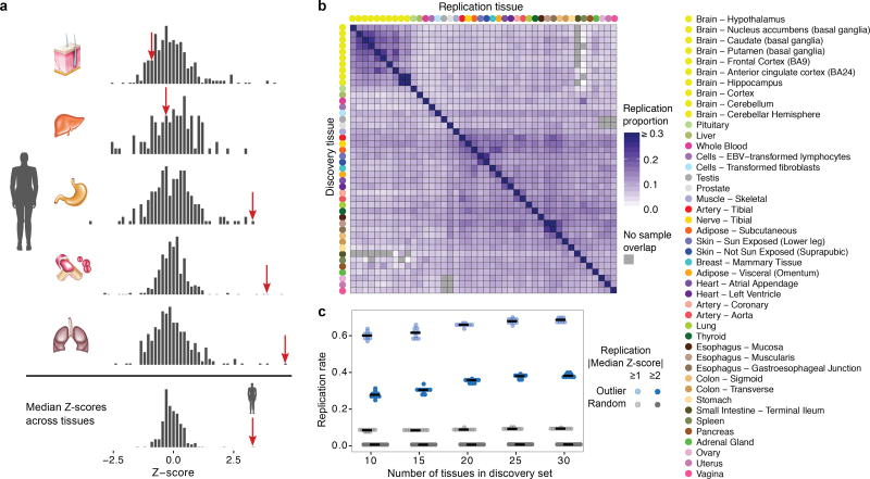
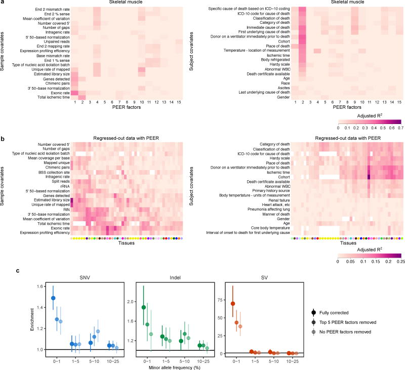
Our analysis focused on individuals with extremely high or low expression of a particular gene compared with the population, using the GTEx v6 release data, which includes RNA-sequencing data for 449 individuals and 44 tissues. We refer to these individuals as gene expression outliers. The GTEx data afford the ability to identify both single-tissue and multi-tissue expression outliers (Fig. 1a), with the latter defined by consistent extreme expression across many tissues (see Methods). To account for broad environmental and technical confounders, we removed hidden factors estimated by PEER¹³ from each tissue prior to outlier discovery (Extended Data Fig. 1 and 2, Supplementary Tables 1 and 2).

Figure 1. Gene expression outliers and sharing between tissues.

(a) A multi-tissue outlier. The individual has extreme expression values for the gene AKR1C4 in multiple tissues (red arrows) and the most extreme median expression value across tissues. (b) Outlier expression sharing between tissues, as measured by the proportion of single-tissue outliers that have |Z-score| ≥ 2 with the same effect direction for the corresponding genes in each replication tissue. Tissues are hierarchically clustered by gene expression. (c) Estimated replication rate of multi-tissue outliers in a constant held-out set of tissues for different sets of discovery tissues.

We identified a single-tissue expression outlier for ≥ 99% of expressed genes in each tissue and a multi-tissue outlier for 4,919 of 18,380 tested genes (27%). Each individual was a single-tissue outlier for a median of 83 genes per tissue compared with a median of 10 genes as a multi-tissue outlier. Single-tissue outliers discovered in one tissue replicated in other tissues at rates up to 33%, with higher rates among related tissues (Fig. 1b, Extended Data Fig. 3). The replication rate for multi-tissue outliers was much higher and increased with the number of tissues used for discovery (Fig. 1c).

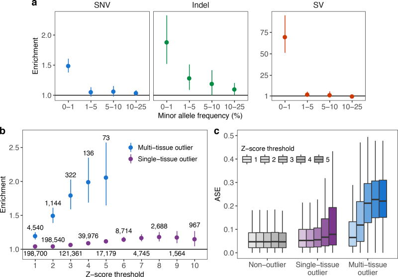
We investigated the influence of rare genetic variation on extreme expression levels, focusing on the individuals of European ancestry with whole genome sequencing data (1,144 multi-tissue outliers). Multi-tissue outliers were strongly enriched for nearby rare variants. The enrichment was most pronounced for structural variants (SVs) as previously described¹⁴, and greater for short insertions and deletions (indels) than for single nucleotide variants (SNVs) (Fig 2a, Extended Data Fig. 4). As most rare variants are heterozygotes, expression outliers driven by rare variants in cis should exhibit allele-specific expression (ASE). Both single-tissue and multi-tissue outliers were significantly enriched for ASE compared with non-outliers (see Methods; two-sided Wilcoxon rank sum tests, each nominal P < 2.2 × 10⁻¹⁶; Fig. 2c). For underexpression outliers with exonic rare variants, the rare allele was generally underexpressed with respect to the common allele and conversely so for overexpression outliers, consistent with the rare variant causing the effect (two-sided Wilcoxon rank sum tests, each nominal P < 4.0 × 10⁻⁸; Extended Data Fig. 5a). The enrichment for rare variants and ASE was stronger for multi-tissue outliers than for single-tissue outliers (Fig. 2b,c, Extended Data Fig. 6a), especially at higher Z-score thresholds.

Figure 2. Enrichment of rare variants and ASE in outliers.

(a) Enrichment of SNVs, indels, and SVs within 10 kb of the TSS among outliers. For each frequency stratum, we calculated enrichment as the relative risk of having a nearby rare variant given the outlier status (see Methods). Bars indicate 95% Wald confidence intervals. (b) Rare SNV enrichments at increasing Z-score thresholds. Text labels indicate the number of outliers at each threshold. (c) ASE, measured as the magnitude of the difference between the reference-allele ratio and the null expectation of 0.5. The non-outlier category is defined in the Methods.

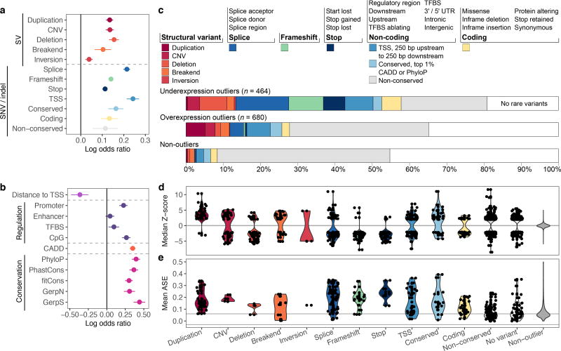
To characterize the properties of rare variants correlated with large changes in gene expression, we assessed the enrichment of different classes of variant types in outliers compared with non-outliers (Supplementary Table 3a). Outliers were enriched, in order of significance, for SVs, variants near splice sites, introducing frameshifts, at start or stop codons, near the transcription start site (TSS), and in conserved regions (Fig. 3a). Variants in coding regions contributed disproportionately to outlier expression; enrichments weakened for all variants types (SNVs, indels, and SVs) when excluding exonic regions (Extended Data Fig. 6b). Additionally, 90% of stop-gain and frameshift variants were predicted to trigger nonsense-mediated decay in outliers, suggesting a biological mechanism for these cases.

Figure 3. Stratification of multi-tissue outliers by rare variant classes.

We considered rare variants in the gene body and within 10 kb of the gene (200 kb for SVs and enhancers). (a) Enrichment of disjoint variant classes among outliers calculated as log odds ratio with 95% Wald confidence intervals. (b) Enrichment of functional annotations for rare SNVs. (c) Proportion of genes with an outlier potentially explained by each rare variant class. (d) Distribution of median Z-scores for each variant class. (e) For each variant class, distribution of ASE (see Methods) averaged across tissues. Grey lines mark the median values among non-outliers.

We also tested the relationship between outlier gene expression and functional annotations. Multi-tissue outliers were strongly enriched for variants in promoter or CpG-rich regions and had variants with higher conservation^15–18 and CADD¹⁹ scores than non-outliers. We observed weaker enrichment in enhancers and transcription factor binding sites (Fig. 3b, Extended Data Fig. 7). Combining all classes of variation, other than non-conserved non-coding rare variants (excluded as less likely candidates for causal effects), we observed that 58% of underexpression and 28% of overexpression outliers had rare variants near the relevant gene, compared with 8% for non-outliers (Fig. 3c). Overexpression outliers were more common overall, potentially because detection of underexpression outliers for very low expression genes is inherently limited (Extended Data Fig. 5b). Overexpression outliers were also less enriched for functionally annotated rare variants (Extended Data Fig. 5c). Some variant classes had strong directionality concordant with their expected impact: duplications caused overexpression, while deletions, start and stop codon variants, and frameshifts coincided with underexpression (Fig. 3d). We also observed strong ASE for outliers carrying all classes except non-conserved variants (Fig. 3e).

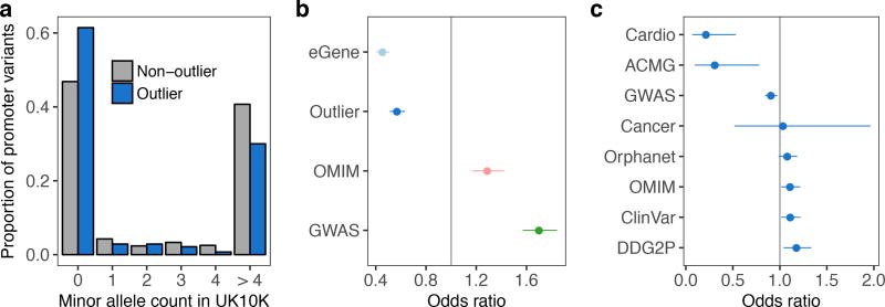
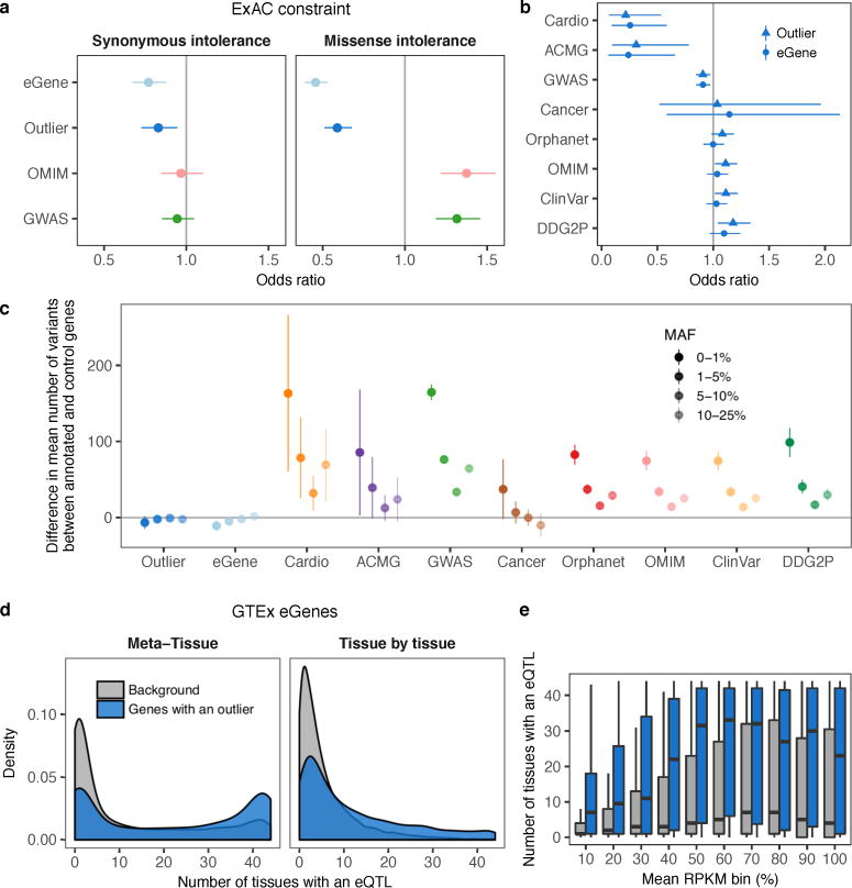
We hypothesized that functional, large-effect rare variants have been under recent selective pressure. As expected, we found that rare promoter variants in outliers were significantly less frequent in the UK10K cohort of 3,781 individuals³ than those from non-outliers for the same genes (two-sided Wilcoxon rank sum test, P = 0.0060; Fig. 4a). Additionally, genes intolerant to loss-of-function and missense mutations were depleted of both multi-tissue outliers and multi-tissue eQTLs (Fisher’s exact test, all P < 2 × 10⁻¹⁵; Fig. 4b, Extended Data Fig. 8a). We observed a similar depletion in two curated disease gene lists—genes involved in heritable cardiovascular disease (Cardio) and genes in the ACMG guidelines for incidental findings²⁰—but not in broader gene lists (Fig. 4c; Extended Data Fig. 8b,c). Genes with a multi-tissue outlier were more likely to have a multi-tissue eQTL (two-sided Wilcoxon rank sum test, P < 2.2 × 10⁻¹⁶; Extended Data Fig. 8d,e), suggesting influence of both rare and common regulatory variation for some genes. However, we found evidence that genes with outliers were more constrained than genes with multi-tissue eQTLs as they harbored less missense and loss-of-function variation (Tukey’s range test, missense Z-score P = 0.0070, probability of loss-of-function intolerance score P = 0.032; Fig. 4b, Extended Data Fig. 8a). This suggests that outlier expression analysis can yield unique insight into constraint on gene regulation.

Figure 4. Evolutionary constraint of genes with multi-tissue outliers.

(a) Distributions of UK10K minor allele frequencies for promoter SNVs in outlier and non-outlier individuals at genes with multi-tissue outliers. (b) Odds ratio of being intolerant to loss-of-function variants for genes with multi-tissue outliers, genes with shared eQTLs (eGenes), genes reported in the GWAS catalog, and OMIM genes. (c) Odds ratio of a gene having a multi-tissue outlier for each of eight sets of genes involved in complex traits or diseases. In (b) and (c) bars represent 95% confidence intervals (Fisher’s exact test).

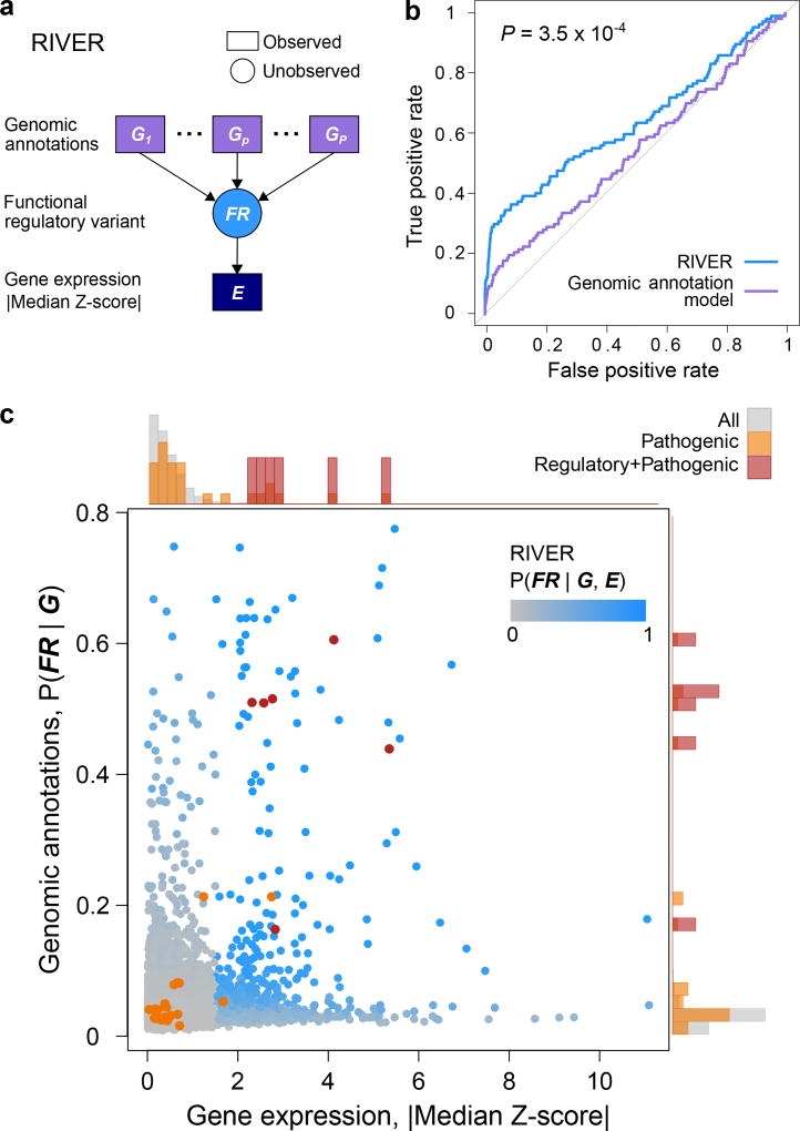
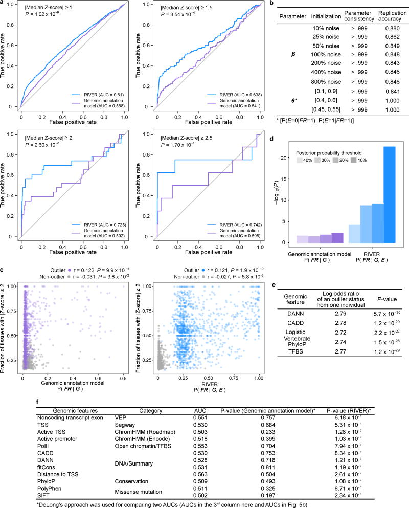
Next, we sought to prioritize rare variants in each individual genome by their predicted impact on regulation of gene expression. We developed RIVER (RNA-Informed Variant Effect on Regulation), a statistical method including a Bayesian model that jointly analyzes genome and transcriptome data from the same individual to estimate the probability that a variant has regulatory impact (https://bioconductor.org/packages/release/bioc/html/RIVER.html, see Methods). RIVER uses a generative model that assumes that genomic annotations (Supplementary Table 3b) determine the prior probability that a variant is a functional regulatory variant, in terms of influence on gene expression, which in turn influences whether nearby genes are likely to display outlier levels of expression (Fig. 5a). RIVER does not require a labeled set of functional/non-functional variants; rather it derives its power from identifying expression patterns that coincide with predictive genomic annotations.

Figure 5. Performance of RIVER for prioritizing functional regulatory variants.

(a) RIVER probabilistic graphical model (see Methods). (b) Predictive power of RIVER compared with an L2-regularized logistic regression model using only genomic annotations. Accuracy was assessed using held-out individuals sharing the same rare SNVs as observed individuals (AUCs compared with DeLong’s approach²⁹). (c) Distribution of RIVER scores (shades of blue) as a function of expression and genomic annotation scores. The distributions of variant categories across expression and genomic annotation scores are shown as histograms aligned opposite the corresponding axes.

We trained RIVER on the GTEx V6 cohort, and evaluated the model on held out pairs of individuals who shared the same rare variants. We then computed the RIVER score (the posterior probability of having a functional regulatory variant) for one individual, using both expression and genomic data, and assessed the accuracy with respect to the second individual’s held-out expression levels (see Methods). Incorporating expression data significantly improved prediction compared with a model that uses genomic annotations alone (AUCs 0.64 and 0.54, respectively, P = 3.5 × 10⁻⁴; Fig. 5b; Extended Data Fig. 9a,b), and RIVER learned, unsupervised, to prioritize variants supported by both genomic annotations and extreme expression levels across tissues (Fig. 5c, Extended Data Fig. 9c). ASE was also enriched among the top RIVER instances compared with the genomic annotation model (Extended Data Fig. 9d). Finally, even after accounting for the most informative genomic annotations or summary scores, personal expression data was highly informative of rare variant effects (average log odds ratio 2.76; Extended Data Fig. 9e,f).

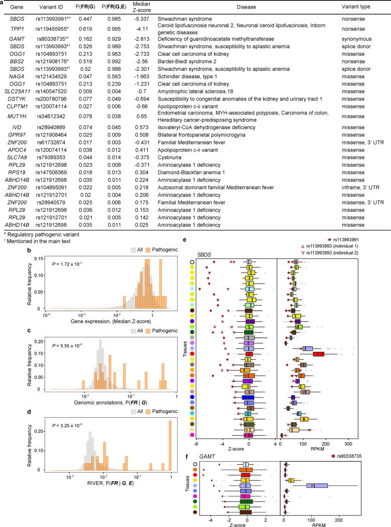
RIVER can be used to predict regulatory effects on gene expression and aid in prioritization amongst disease associated variants. To investigate this potential, we evaluated 27 pathogenic variants from ClinVar²¹ present in 21 GTEx donors (Fig. 5c, Extended Data Fig. 10a). Overall, pathogenic variants had RIVER scores higher than background variants (two-sided Wilcoxon rank sum test, P = 3.3 × 10⁻⁹; Extended Data Fig. 10b–d), and the six that were likely regulatory (those not annotated as missense or coding indel) scored in the 99.9^th percentile. Evaluated in detail, several cases illustrated that rare disease-causing variants can have a regulatory impact evident from RNA-seq data, even from healthy individuals harboring those variants (where they are often heterozygous; Extended Data Fig. 10e,f). Note that RIVER trained on healthy cohorts such as GTEx can then be directly applied to new cohorts including disease samples.

To experimentally validate a subset of the variants identified through outlier analysis, we used CRISPR/Cas9 mediated genome editing^22,23. In K562 cells, we tested six SNVs and matched controls in transcribed regions of genes with an outlier (see Methods; Extended Data Fig. 11a,b), and compared the allelic ratios between mRNA and genomic DNA (gDNA), an internal control. All variants tested were in underexpression outliers and were therefore expected to decrease expression. Two variants were excluded due to low cDNA and gDNA total reads counts. The four remaining SNVs in outliers all showed lower proportions of the alternate (installed) allele in the cDNA compared with gDNA, confirming that these variants decreased expression (Extended Data Fig. 11c).

In summary, by combining data across multiple tissues, we curated a set of gene expression outliers that replicated at higher rates and showed stronger rare variant enrichments than those from any single tissue. We found that rare structural variants, frameshift indels, coding variants, and variants near the transcription start site were most likely to have large effects on expression. However, our ability to characterize the genetic basis of multi-tissue outliers remains incomplete. Outliers without an underlying rare variant in our analysis may be due to variants in more distal regions or in annotations we did not consider, or may be attributable to residual technical or environmental effects.

Although genetic variant interpretation remains challenging, RIVER demonstrates the value of incorporating personal gene expression data to examine the influence of rare variants on expression that may be uncertain from sequence alone. Our results suggest a general approach that can be applied to studies that supplement genome sequencing with other molecular phenotypes, such as methylation^24–26 and histone modification^27,28. We anticipate that such integrative approaches will be essential for effective interpretation of genome-wide genetic variation on a personalized level.

Methods

Study population

All human subjects were deceased donors. Informed consent was obtained for all donors via next-of-kin consent to permit the collection and banking of de-identified tissue samples for scientific research. The research protocol was reviewed by Chesapeake Research Review Inc., Roswell Park Cancer Institute’s Office of Research Subject Protection, and the institutional review board of the University of Pennsylvania. We used the RNA-seq, allele-specific expression, and whole genome sequencing (WGS) data from the v6 release of the GTEx project. The generation of these data is described in Supplementary Information sections 3 and 5 of the main GTEx Consortium publication¹².

Correction for technical confounders

We restricted our expression analyses to the 449 individuals and 44 tissues for which sex and the top three genotype principal components (PCs), which capture major population stratification, were available. For each tissue, we log₂-transformed all expression values (log₂(RPKM + 2)). We then standardized the expression of each gene to prevent shrinkage of outlier expression values caused by quantile normalization. To remove unmeasured batch effects and other confounders, for each tissue separately, we estimated hidden factors using PEER¹³ on the transformed expression values. In each tissue, we defined expressed genes and corrected for the same number of PEER factors as in the GTEx eQTL analyses (see Supplementary Information sections 5.5 and 5.6 of the main GTEx Consortium publication¹²). We regressed out the PEER factors, the top three genotype principal components, and sex (where appropriate) from the transformed expression data for each tissue using the following linear model:

$${\mathit{Y}}_{\mathit{g}}={\mu }_g\mathbf{1}+\sum _{n=1}^N{\alpha }_{g,n}{\mathit{P}}_n+\sum _{k=1}^3{\beta }_{g,k}{\mathit{G}}_k+{\gamma }_g\mathit{S}+{\mathit{\epsilon }}_{\mathit{g}}$$

where Y_g is the transformed expression in the given gene g, μ_g is the mean expression level for the gene, P_n is the n^th PEER factor, G₁, G₂, G₃ are the top three genotype PCs, and S is the sex covariate. We assumed the residual vector ε_g follows the multivariate normal distribution ε_g ~ N(0, σ²I). Finally, we standardized the expression residuals ε_g for each gene, which yielded Z-scores.

To better understand the effect of PEER correction on the removal of technical and biological confounders, we compared the PEER factors in each tissue separately to pre-collected sample and subject covariates. We considered the subset of covariates with >50 observations in at least 31 tissues, where we first selected covariates with more than one unique entry in each tissue. For categorical covariates, we only considered categories with more than 20 observations. For each PEER factor and each covariate, we fit a linear model with the PEER factor as the response and the covariate as the predictor. From this model, we computed the proportion of that PEER factor’s variance explained by the covariate as the adjusted R²:

$$\text{Adjusted }{R}^2=R^2-[(1-R^2)·\frac{p}{n-p-1}]$$

where p and n are the number of parameters and samples, respectively, and $R^2=\frac{{\mathit{\text{SS}}}_T-{\mathit{\text{SS}}}_R}{{\mathit{\text{SS}}}_T}$. SS_T and SS_R refer to the total and residual sums of squares, respectively.

To quantify the degree to which each covariate was captured by the combination of all PEER factors, genotype PCs, and sex (where appropriate) for each tissue, we considered the expression component regressed out from the uncorrected data:

$${\mathit{W}}_g={\mathit{Y}}_g-{\mathit{\epsilon }}_g$$

For each covariate, we then fit a linear model with W_g as the response and the covariate as the predictor. We assessed the proportion of the variance of W_g explained by each covariate by computing the adjusted R² for the covariate across all genes. We used the formula above, but summed across all genes to compute SS_T and SS_R.

To assess the impact of PEER correction on rare variant enrichment, we also tried removing either the top five PEER factors for each tissue or no PEER factors. We then performed multi-tissue outlier calling and tested the enrichment of rare and common variants in the two partially corrected datasets (see Methods section “Enrichment of rare and common variants near outlier genes”).

Single-tissue and multi-tissue outlier discovery

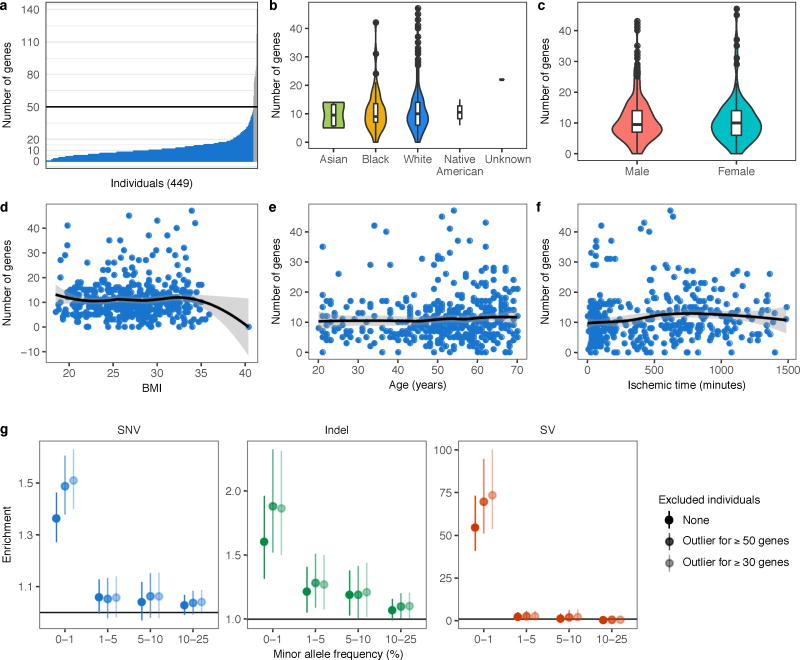
Single-tissue and multi-tissue outlier calling was restricted to autosomal lincRNA and protein coding genes. For each tissue, an individual was called a single-tissue outlier for a particular gene if that individual had the largest absolute Z-score and the absolute value was at least two. For each gene, the individual with the most extreme median Z-score taken across tissues was identified as a multi-tissue outlier for that gene provided the absolute median Z-score was at least two. Therefore, each gene had at most one single-tissue outlier per tissue and one multi-tissue outlier. Under this definition an individual could be an outlier for multiple genes. In addition, we only tested for multi-tissue outliers among individuals with expression measurements for the gene in at least five tissues. To reduce cases where non-genetic factors may cause widespread extreme expression, we removed eight individuals that were multi-tissue outliers for 50 or more genes from all downstream analyses, including before single-tissue outlier discovery. Removing these individuals with extreme expression across many genes improved our rare variant enrichments, but the precise threshold mattered less (Extended Data Fig. 2g). We chose the threshold of 50 to strike a balance between removing extreme individuals while not excluding a large proportion of our cohort.

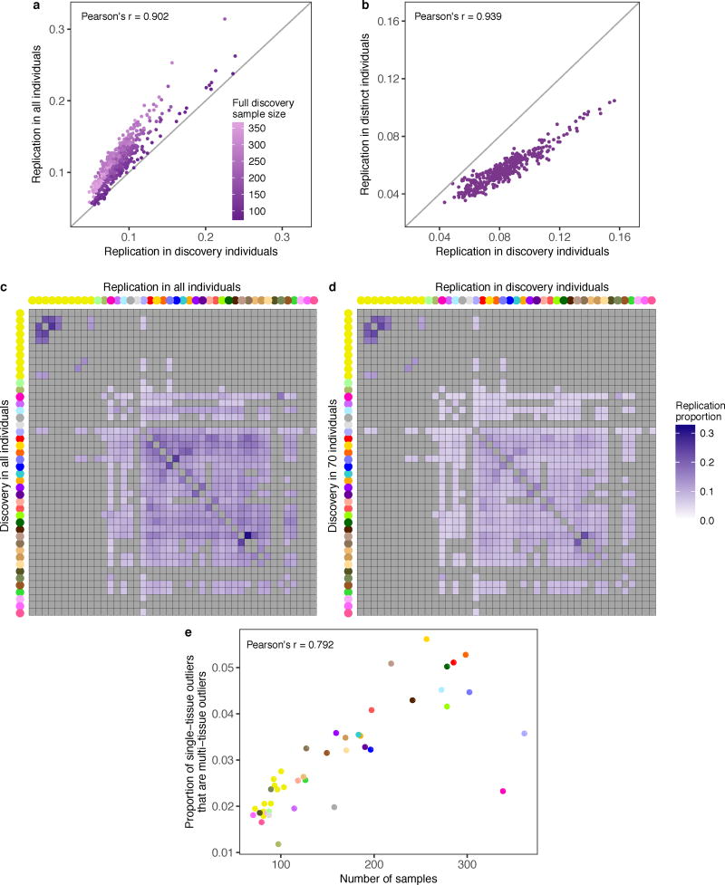
Replication of expression outliers

We calculated the proportion of single-tissue outliers discovered in one tissue that had |Z-score| ≥ 2 with the same direction of effect for the same gene in the replication tissue. Since certain groups of tissues were sampled in a specific subset of individuals, we evaluated the extent to which replication was influenced by the size and the overlap of the discovery and replication sets. We repeated the replication analysis with the discovery and replication in exactly 70 overlapping individuals for each pair of tissues with enough samples and compared the replication patterns to those obtained by using all individuals. To estimate the extent to which individual overlap biased replication estimates, for each pair of tissues with sufficient samples, we defined three disjoint groups of individuals: 70 individuals with data for both tissues, 69 distinct individuals with data in the first tissue, and 69 distinct individuals with data in the second tissue. We discovered outliers in the first tissue using the shared set of individuals then tested for replication using the same individuals in the second tissue. Then, for each gene, we added the identified outlier to the distinct set of individuals and tested the replication again in the second tissue. We repeated the process running the discovery in the second tissue and the replication in the first one. We compared the replication rates when using the same or different individuals for the discovery and replication.

We assessed the confidence of our multi-tissue outliers using cross-validation. We separated the tissue expression data randomly into two groups: a discovery set of 34 tissues and a replication set of 10 tissues. For t = 10, 15, 20, 25, and 30, we randomly sampled t tissues from the discovery set and performed outlier calling as described above. Due to incomplete tissue sampling, the number of tissues supporting each outlier is at least five but less than t. We computed the replication rate as the proportion of outliers in the discovery set with |median Z-score| ≥ 1 or 2 in the replication set. We set no restriction on the number of tissues required for testing in the replication set. To calculate the expected replication rate, we randomly selected individuals in the discovery set with at least five tissues that expressed the gene and computed the replication rate. We repeated this process 10 times for each discovery set size.

Quality control of genotypes and rare variant definition

We restricted our rare variant analyses to individuals of European descent, as they constituted the largest homogenous population within our dataset. We considered only autosomal variants that passed all filters in the VCF (those marked as PASS in the Filter column). Minor allele frequencies (MAF) within the GTEx data were calculated from the 123 individuals of European ancestry with whole genome sequencing data (average coverage 30×). The MAF was the minimum of the reference and the alternate allele frequency where the allele frequencies of all alternate alleles were summed together. Rare variants were defined as having MAF ≤ 0.01 in GTEx, and for SNVs and indels we also required MAF ≤ 0.01 in the European population of the 1000 Genomes Project Phase 3 data³⁰. To ensure that population structure among the individuals of European descent was unlikely to confound our results, we verified that the allele frequency distribution of rare variants included in our analysis (within 10 kb of a protein coding or lincRNA gene, see below) was similar for the five European populations in the 1000 Genomes project (Extended Data Fig. 4d).

Enrichment of rare and common variants near outlier genes

We assessed the enrichment of rare SNVs, indels, and SVs near outlier genes. Proximity was defined as within 10 kb of the TSS for most analyses. For Fig. 3 and Extended Data Figs. 5, 7 and 8, we included all variants within 10 kb of the gene, including the gene body, to also capture coding variants. In Fig. 3 and Extended Data Fig. 5 and 8, we extended the window to 200 kb for enhancers and SVs. For each gene with an outlier, we chose the remaining set of individuals tested for outliers at the same gene as non-outlier controls. We only considered genes that had both an outlier and at least one control. We stratified variants of each class into four minor allele frequency bins (0–1%, 1–5%, 5–10%, 10–25%) to compare the relative enrichments of rare and common variants. We also assessed the enrichment of SNVs at different Z-score cutoffs. Enrichment was defined as the ratio of the proportion of outliers with a variant whose frequency lies within the range to the corresponding proportion for non-outliers. This enrichment measure is equivalent to the relative risk of having a nearby rare variant given outlier status. We used the asymptotic distribution of the log relative risk to obtain 95% Wald confidence intervals. Within our set of European individuals, we observed some individuals with minor admixture that had relatively more rare variants than the rest (Extended Data Fig. 1b). We confirmed that inclusion of these admixed individuals did not substantially affect our results (Extended Data Fig. 1c). We also calculated rare variant enrichments when restricting to variants outside protein-coding and lincRNA exons in Gencode v19 annotation (extending internal exons by 5 bp to capture canonical splice regions).

To measure the informativeness of variant annotations, we used logistic regression to model outlier status as a function of the feature of interest, which yielded log odds ratios with 95% Wald confidence intervals. Note that for the feature enrichment analysis in Fig. 3b and Extended Data Fig. 7, we required that outliers and their gene-matched non-outlier controls have at least one rare variant near the gene. We standardized all features, including binary features, to facilitate comparison between features of different scale. We also calculated the proportion of overexpression outliers, underexpression outliers and non-outliers with a rare variant near the gene (within 10 kb for SNVs and indels and 200 kb for SVs). To each outlier instance, we assigned at most one of the 12 rare variant classes we considered (Supplementary Table 3a). If an outlier had rare variants from multiple classes near the relevant genes, we selected the class that was most significantly enriched among outliers.

Annotation of variants

We obtained SV anntoations from Chiang et al.¹⁴ and computed features for rare SNVs and indels using three primary data sources: Epigenomics Roadmap³¹, CADD v1.2¹⁹, and VEP v80³². Promoter and enhancer annotation tracks were obtained from the Epigenomics Roadmap Project (http://www.broadinstitute.org/~meuleman/reg2map/HoneyBadger2_release/). We mapped 28 unique tissues in the GTEx Project to 19 tissue groups in the Roadmap Project. Using these annotations, for each individual, we assessed whether each SNV or indel overlapped a promoter or enhancer region in at least one of the 19 Roadmap tissue groups. Features including conservation^15–18, transcription factor binding, and deleteriousness were extracted from the full annotation tracks of the CADD v1.2 release (downloaded 15/05/2015; http://cadd.gs.washington.edu/download). Finally, we obtained protein-coding and transcription-related annotations from VEP. This information was provided in the GTEx v6 VCF file. Stop-gain and frameshift variants annotated as high-confidence loss-of-function variants by LOFTEE were assumed to trigger nonsense-mediated decay. We generated gene-level features described in Supplementary Table 3.

Allele-specific expression (ASE)

We only considered sites with at least 30 total reads and at least five reads supporting each of the reference and alternate alleles. To minimize the effect of mapping bias, we filtered out sites that showed mapping bias in simulations³³, that were in low mappability regions (ftp://hgdownload.cse.ucsc.edu/gbdb/hg19/bbi/wgEncodeCrgMapabilityAlign50mer.bw), or that were rare variants or within 1 kb of a rare variant in the given individual (the variants were extracted from the GTEx exome sequencing data described in section 4 of the main GTEx consortium publication¹²). The first two filters were provided in the GTEx ASE data release. The third filter was applied to eliminate potential mapping artifacts that mimic genetic effects from rare variants. We measured ASE at each testable site as the absolute deviation of the reference allele ratio from 0.5. For each gene, all testable sites in all tissues were included. We compared ASE in single-tissue and multi-tissue outliers at different Z-score thresholds to non-outliers using two-sided Wilcoxon rank sum tests. To obtain a matched background, we only included a gene in the comparison when ASE data existed for both the outlier individual and at least one non-outlier. In the case of single-tissue outliers, we also required the tissue to match between the outlier and the non-outlier. All individuals that were neither multi-tissue outliers for the given gene nor single-tissue outliers for the gene in the corresponding tissue were included as non-outliers.

In cases where outliers had rare coding variants in the gene, if the rare variants were causing the extreme expression in cis, we expected to see ASE at the rare variant matching the direction of the effect. For underexpression outliers, we expected the (rare) minor allele to be underexpressed compared with the major allele. For overexpression outliers, we expected the minor allele to be overexpressed. To test this, we used the same filters as above, but looked exclusively at rare variants (instead of excluding them). We measured ASE as the minor allele ratio: the number of reads supporting the minor allele over the total number of reads.

We also used ASE to evaluated performance of both the genomic annotation model and RIVER (see below) by testing the association between allelic imbalance and model predictions using Fisher's Exact Test. Here, we defined allelic imbalance as the top 10% of the median absolute deviation, across tissues, of the reference allele ratio from 0.5.

Allele frequency measurements in UK10K

UK10K³ VCF files of whole genome cohorts were downloaded from https://www.ebi.ac.uk. We merged the Avon Longitudinal Study of Parents and Children (ALSPAC) EGAS00001000090 and the Department of Twin Research and Genetic Epidemiology (TWINSUK) EGAS00001000108 datasets for a total of 3,781 individuals. We counted the occurrence of all rare GTEx SNVs in Epigenomics Roadmap-annotated promoter regions among the UK10K samples. GTEx variants absent from the UK10K cohorts were assigned a count of 0.

Definition of multi-tissue eGenes

We defined multi-tissue eGenes using two approaches. For the tissue-by-tissue approach, we obtained lists of significant eGenes (q-value ≤ 0.05) for each of the 44 tissues from the GTEx v6p release. The second approach used cis-eQTLs with shared effects across tissues estimated by the RE2 model of the Meta-Tissue software³⁴, as described in the main consortium manuscript¹². We chose for each gene the variant with the lowest nominal P-value from the RE2 model. We then determined the number of tissues in which this variant-gene pair showed a cis-eQTL effect (m-value ≥ 0.9³⁴). For each of the 18,380 genes tested for multi-tissue outliers, we calculated the number of tissues in which the gene appeared as a significant eGene (tissue-by-tissue approach) or had a shared eQTL effect (Meta-Tissue approach). To show that the enrichment of outlier genes as multi-tissue eGenes was not confounded by gene expression level, using the Meta-Tissue results, we stratified genes tested for multi-tissue outliers into RPKM deciles and repeated the comparison between genes with and without a multi-tissue outlier. When comparing the enrichment for eGenes among constrained and disease gene lists, we classified the top n Meta-Tissue eGenes (ranked by nominal P-value from the RE2 model) as multi-tissue eGenes and considered the remaining genes as background. We selected n to match the umber of multi-tissue outliers in the comparison.

Evolutionary constraint of genes with multi-tissue outliers

We obtained gene-level estimates of evolutionary constraint from the Exome Aggregation Consortium³⁵ (http://exac.broadinstitute.org/, ExAC release 0.3). We intersected the 17,351 autosomal lincRNA and protein coding genes with constraint data from ExAC with the 18,380 genes tested for multi-tissue outliers from GTEx, yielding 14,379 genes for further analysis (3,897 and 10,482 genes with and without a multi-tissue outlier, respectively). We examined three functional constraint scores from the ExAC database: synonymous Z-score, missense Z-score, and probability of loss-of-function intolerance (pLI). Synonymous- and missense-intolerant genes were defined as those with corresponding Z-scores above the 90^th percentile. We defined loss-of-function intolerant genes as those with a pLI score above 0.9, following the guidelines provided by the ExAC consortium. We calculated odds ratios and 95% confidence intervals for the enrichment of genes with multi-tissue outliers in these lists using Fisher’s exact test. We repeated this analysis for three other gene sets: 19,182 multi-tissue eGenes from GTEx v6p defined using Meta-Tissue, 9,480 reported GWAS genes from the NHGRI-EBI catalog³⁶ (http://www.ebi.ac.uk/gwas accessed 30/11/2015), and 3,576 OMIM genes (http://omim.org/ accessed 26/5/2016).

We tested for a difference in the mean constraint for genes with multi-tissue outliers and genes with multi-tissue eQTLs using ANOVA. For each constraint score in ExAC, we treated the score for each gene as the response and the status of the gene as having a multi-tissue outlier and/or a multi-tissue eQTL as a categorical predictor with four classes. After fitting the model, we performed Tukey’s range test to determine whether there was a significant difference in the mean constraint between genes with a multi-tissue outlier but no multi-tissue eQTL and genes with a multi-tissue eQTL but no multi-tissue outlier.

Overlap of genes with multi-tissue outliers and disease genes

We examined the enrichment of genes with multi-tissue outliers in eight disease gene lists: the GWAS catalog and OMIM (described above) as well as ClinVar (6,279 genes; http://www.ncbi.nlm.nih.gov/clinvar/), OrphaNet (3,451 genes; http://www.orpha.net/), ACMG²⁰ (58 genes; http://www.ncbi.nlm.nih.gov/clinvar/docs/acmg/), Developmental Disorders Genotype-Phenotype³⁷ (DDG2P; 1693 genes; http://www.ebi.ac.uk/gene2phenotype/), and two curated gene lists of 86 cardiovascular disease genes and 55 cancer genes (described below). We computed odds ratios and 95% confidence intervals using Fisher’s exact test to compare each disease gene list to the genes with multi-tissue outliers and repeated the comparison for genes with multi-tissue eQTLs.

Heritable cancer predisposition and heritable cardiovascular disease gene lists were curated by local experts in clinical and laboratory-based genetics in the two respective areas (Stanford Medicine Clinical Genomics Service, Stanford Cancer Center's Cancer Genetics Clinic, and Stanford Center for Inherited Cardiovascular Disease). Genes were included if both the clinical and laboratory-based teams agreed there was sufficient published evidence to support using variants in these genes in clinical decision making.

For each of the eight disease gene lists above and for genes with multi-tissue outliers or multi-tissue eQTLs, we computed the number of variants (SNVs and indels within 10 kb and SVs within 200 kb of the gene, including the gene body) at each gene in the 123 individuals of European ancestry with WGS data. For each gene list and for each MAF bin (0–1%, 1–5%, 5–10%, 10–25%), we compared the mean number of variants near genes in the list to the mean number near all other annotated autosomal protein coding and lincRNA genes using a two-sided t-test.

RIVER integrative model for predicting regulatory effects of rare variants

RIVER (RNA-Informed Variant Effect on Regulation) is a hierarchical Bayesian model that predicts the regulatory effects of rare variants by integrating gene expression with genomic annotations. The RIVER model consists of three layers: a set of nodes G = G₁ … G_P in the topmost layer representing P observed genomic annotations over all rare variants near a particular gene, a latent binary variable FR in the middle layer representing the unobserved functional regulatory status of the rare variants, and one binary node E in the final layer representing expression outlier status of the nearby gene. We model each conditional probability distribution as follows:

$$\mathit{\text{FR}}|\mathit{G}~\text{Bernoulli}(\psi ),\psi ={\text{logit}}^{-1}(\mathit{\beta }\prime \mathit{G})$$

$$E|\mathit{\text{FR}}~\text{Categorical}({\mathit{\theta }}_{\mathit{\text{FR}}})$$

$${\beta }_i~𝒩(0,\frac{1}{\lambda })$$

$${\mathit{\theta }}_{\mathit{\text{FR}}}~\text{Beta}(C,C)$$

with parameters β and θ and hyper-parameters λ and C.

Because FR is unobserved, the RIVER log-likelihood objective over instances n = 1, …, N ${\sum }_{n=1}^N\text{log }{\sum }_{{\mathit{\text{FR}}}_n=0}^{1}P(E_n,{\mathit{G}}_n,{\mathit{\text{FR}}}_n|\mathit{\beta },\mathit{\theta })$ is non-convex. We therefore optimize model parameters via Expectation-Maximization³⁸ (EM) as follows:

In the E-step, we compute the posterior probabilities (ω_n⁽ⁱ⁾) of the latent variables FR_n given current parameters and observed data. For example, at the ith iteration, the posterior probability of FR_n = 1 for the n^th instance is

$${\omega }_{1n}^{(i)}=P({\mathit{\text{FR}}}_n=1|{\mathit{G}}_n,{\mathit{\beta }}^{(i)},E_n,{\mathit{\theta }}^{(i)})=\frac{P({\mathit{\text{FR}}}_n=1|{\mathit{G}}_n,{\mathit{\beta }}^{(i)})P(E_n|{\mathit{\text{FR}}}_n=1,{\mathit{\theta }}^{(i)})}{{\sum }_{{\mathit{\text{FR}}}_n=0}^{1}P({\mathit{\text{FR}}}_n|{\mathit{G}}_n,{\mathit{\beta }}^{(i)})·P(E_n|{\mathit{\text{FR}}}_n,{\mathit{\theta }}^{(i)})}$$

$${\omega }_{0n}^{(i)}=1-{\omega }_{1n}^{(i)}.$$

In the M-step, at the ith iteration, given the current estimates ω⁽ⁱ⁾, the parameters (β^{(i + 1)}*) are estimated as

$$\underset{{\mathit{\beta }}^{(\mathit{i}+\mathbf{1})}}{\text{argmax}}{\sum }_{n=1}^N{\sum }_{{\mathit{\text{FR}}}_n=0}^1\text{log }(p({\mathit{\text{FR}}}_n|{\mathit{G}}_n,{\mathit{\beta }}^{(i+1)}))·{\omega }_{\mathit{\text{FR}},n}^{(i)}-\frac{\lambda }{2}{\Vert {\mathit{\beta }}^{(i+1)}\Vert }_2,$$

where λ is an L2 penalty hyper-parameter derived from the Gaussian prior on β.

The parameters θ get updated as:

$${\theta }_{\mathit{\text{st}}}^{(i+1)}=\sum _{\mathit{n}=\mathbf{1}}^{\mathit{N}}\mathrm{I}(E_n=t)·{\omega }_{s,n}^{(i)}+C,$$

where I is an indicator operator, t is the binary value of expression E_n, s is the possible binary values of FR_n, and C is a pseudo count derived from the Beta prior on θ. The E and M steps are applied iteratively until convergence.

RIVER application to the GTEx cohort

As input, RIVER requires a set of genomic features G and a set of corresponding expression outlier observations E, each over instances of individual and gene pairs. Using the variant annotations described above, we generated site-level genomic features for the 116 European individuals with GTEx WGS data that had fewer than 50 multi-tissue outliers. We then collapsed these features for all rare SNVs within 10 kb of each TSS to generate gene-level features described in Supplementary Table 3b. This produced a matrix of genomic features G of size (116 individuals × 1,736 genes) × (112 genomic features), where we standardized features before use. For the values E, we defined any individual with |median Z-score| ≥ 1.5 as an outlier if expression was observed in at least five tissues; the remaining individuals were labeled as non-outliers for the gene. We used this more lenient threshold in order to obtain a sufficiently large set of outliers for robust training and testing. In total, we extracted 48,575 instances where an individual had at least one rare variant within 10 kb of the TSS of a gene.

To train and evaluate RIVER on the GTEx cohort, we used the 3,766 instances of individual and gene pairs where two individuals had the same rare SNVs near a particular gene. We held out those instances and trained RIVER parameters with the remaining instances. RIVER requires two hyper-parameters λ and C. To select λ, we first applied an L2-regularized multivariate logistic regression with features G and response variable E, selecting lambda with the minimum squared error via 10-fold cross-validation (we selected λ = 0.01). We selected C = 50, informed simply by the total number of training instances available, as validation data was not available for extensive cross-validation. Initial parameters for EM were set to θ = (P(E = 0 | FR = 0), P(E = 1 | FR = 0), P(E = 0 | FR = 1), P(E = 1 | FR = 1)) = (0.99, 0.01, 0.3, 0.7) and β from the multivariate logistic regression above, although different initializations did not significantly change the final parameters (Extended Data Fig. 9b).

The 3,766 held out pairs of instances were used to create a labeled evaluation set. For one of the two individuals from each pair, we estimated the posterior probability of a functional rare variant P(FR | G, E, β, θ). The outlier status of the second individual, whose data was not observed either during training or prediction, was then treated as a “label” of the true status of functional effect FR. Using this labeled set, we compared the RIVER score to the posterior P(FR | G, β) estimated from the plain L2-regualrized multivariate logistic regression model with genomic annotations alone. We produced ROCs and computed AUCs for both models, testing for significant differences using DeLong’s method²⁹. This measure relied on outlier status reflecting the consequences of rare variants. Indeed, pairs of individuals who shared rare variants tended to have highly similar outlier status even after regressing out effects of common variants (Kendall’s tau rank correlation, P < 2.2 × 10⁻¹⁶). We repeated this evaluation, varying the median Z-score threshold used to define outliers, and we also compared RIVER to individual features that were strongly enriched among outliers as well as PolyPhen³⁹ and SIFT⁴⁰.

Supervised model integrating expression and genomic annotation

To assess the information gained by incorporating gene expression data in the prediction of functional rare variants, we applied a simplified supervised approach to a limited dataset. We used the instances where two individuals had the same rare SNVs to create a labeled training set where the outlier status of the second individual was used as the response variable. We then trained a logistic regression model with just two features: 1) the outlier status of the first individual and 2) a single genomic feature value such as CADD or DANN. We estimated parameters from the entire set of rare-variant-matched pairs using logistic regression to determine the log odds ratio and corresponding P-value of expression status as a predictor. While this approach was not amenable to training a full predictive model over all genomic annotations jointly given the limited number of instances, it provided a consistent estimate of the log odds ratio of outlier status. We tested five genomic predictors: CADD¹⁹, DANN⁴¹, transcription factor binding site annotations, PhyloP scores¹⁵, and one aggregated feature: the posterior probability from a multivariate logistic regression model learned with all genomic annotations.

RIVER assessment of pathogenic ClinVar variants

We downloaded variants from the ClinVar database²¹ (accessed 04/05/2015) and searched any of these disease variants within the set of rare variants segregating in the GTEx cohort. Any disease variant reported as pathogenic, likely pathogenic, or a risk factor for disease was considered pathogenic. We further categorized the pathogenic variants as likely regulatory if they were annotated as splice-site variants, synonymous, or nonsense, whereas missense variants were considered unlikely to have a regulatory effect. To explore RIVER scores for those pathogenic variants, all instances were used for training RIVER. We then computed a posterior probability P(FR | G, E, β, θ) for each instance coinciding with a pathogenic ClinVar variant.

Stability of estimated parameters with different parameter initializations

We tried several different initialization parameters for β and θ to explore how this affected the estimated parameters. We initialized a noisy β by adding K% Gaussian noise compared to the mean of β with fixed θ (for K = 10, 20, 50 100, 200, 400, 800). For θ, we fixed P(E = 1 | FR = 0) and P(E = 0 | FR = 0) as 0.01 and 0.99, respectively, and initialized (P(E = 1 | FR = 1), P(E = 0 | FR = 1)) as (0.1, 0.9), (0.4, 0.6), and (0.45, 0.55) instead of (0.3, 0.7) with β fixed. For each parameter initialization, we computed Spearman rank correlations between parameters from RIVER using the original initialization and the alternative initializations. We also investigated how many instances within top 10% of posterior probabilities from RIVER under the original settings were replicated in the top 10% of posterior probabilities under the alternative initializations (Replication accuracy in Extended Data Fig. 9b).

Validation of large-effect rare variants via CRISPR/Cas9 genome editing

To select rare, coding SNVs for validation by CRISPR/Cas9 editing, we first restricted to the (gene, individual, variant) tuples identified in multi-tissue outliers without a rare SV or a rare indel within 200 kb or 10 kb of the gene, respectively. We considered the 116 rare SNVs with a coding consequence for the corresponding gene as annotated by VEP³²; coding annotations included stop gained, stop lost, splice acceptor variant, splice donor variant, start lost, missense variant, splice region variant, stop retained variant, synonymous variant, coding sequence variant, and 5’/3’ UTR variant. Using RNA-seq data from ENCODE, we further restricted our variant list to the 59 SNVs occurring in genes with an average FPKM of at least 10 in K562 cells (ENCODE experiment IDs ENCSR000AEL and ENCSR000AEN)⁴². Finally, we filtered for rare, coding SNVs in (gene, individual) pairs with |median Z-score| > 4 and a RIVER score above the 99.5^th percentile. These filters yielded a final set of 13 rare SNVs from which we chose the six exonic SNVs for testing.

As controls, we selected SNVs present within the same cDNA amplicon region as the corresponding outlier SNV (see details on targeted sequencing below). We first searched for coding SNVs present within these regions in the GTEx cohort that did not occur in the outlier individual. If no SNV could be found satisfying these criteria, we expanded our search for SNVs using the ExAC database (ExAC release 0.3)³⁵. If multiple possible control variants existed for an outlier SNV, we ranked the controls by CADD score¹⁹ and prioritized synonymous variants.

Sequences of single-guide RNAs (sgRNAs) used in the study are listed in Extended Data Fig. 11b. For each variant, a sgRNA and two donor oligonucleotides (with the reference and alternative alleles) were designed such that the PAM was located as close to the variant as possible. The donors were 99 bp long centered on the variant being installed. The variants were installed into K562 cells as previously described^22,23. The K562 cells were those generated previously²³ and were regularly tested for mycoplasma infection. sgRNAs were expressed in the pGH020 (Addgene plasmid #85405) expression vector. For each donor oligonucleotide, K562 cells constitutively expressing a Cas9-BFP protein fusion were electroporated with 3 µg of sgRNA plasmid DNA and 1 µL of 100 µM donor oligonucleotide using the T-016 program on a Lonza Nucleofector 2b. After electroporation, cells were allowed to recover for 5 days. Cells electroporated with the reference and alternative allele donor oligonucleotides were mixed in a 1:1 ratio and grown together for 3 more days to control for differences in culturing conditions. We included cells electroporated with the reference allele to ensure that any changes in expression we observed were not due to the editing process itself. Since the editing efficiency is not 100% and varies between loci, we expect fewer than half the cells to carry the alternative allele and for this proportion to vary by locus. One to two million cells were collected for RNA and genomic DNA extraction.

Genomic DNA was extracted using the QiaAmp DNA mini kit (Qiagen). Total RNA was extracted using QiaShredder and RNeasy Mini kit (Qiagen). Six µg of RNA was converted into cDNA using AMV reverse transcriptase (Promega). cDNA was purified and concentrated with the PCR Purification Kit (Qiagen). PCR primers were designed to generate 300–400 bp amplicons including the variant in either the genomic DNA or cDNA locus. For both genomic DNA and cDNA samples, 400 ng of DNA was amplified in triplicate (technical replicates) using Phusion High-Fidelty polymerase (Fisher) and the amplicon was purified on a 1% TAE agarose gel. The amplicons were then prepared for sequencing using the Nextera XT kit (Illumina) and sequenced together on a NextSeq 500.

Reads were trimmed with cutadapt⁴³ (version 1.13) and aligned using bwa⁴⁴ (version 0.7.12-r1039) allowing no mismatches (bwa aln –n 0), which excluded any reads with indels created during editing. We used custom reference sequences, one each for the reference and alternate alleles of the targeted cDNA and gDNA amplicon regions. Allele counts at the target locus were computed for each sample using samtools pileup as implemented in the R package Rsamtools⁴⁵ (version 1.22.0). Only reads with a minimum mapping quality of 20 were considered. Two of the tested loci amplified poorly in preparation for sequencing, and they had extremely low mapping rates and total read counts over the target locus (median read count across replicates < 400 compared to 281,000 and 397,000 for gDNA and cDNA, respectively, for the remaining loci). As such, we removed these two loci from further analysis. Finally, to assess the effect of each variant on expression, we tested for a significant difference between the cDNA and gDNA alternate allele proportions with a two-sided t-test. We corrected for multiple testing using the Bonferroni procedure.

Code availability

RIVER is available at https://bioconductor.org/packages/release/bioc/html/RIVER.html. Additionally, the code for running analyses and producing the figures throughout this manuscript is available separately (https://github.com/joed3/GTExV6PRareVariation).

Data availability

The GTEx v6 release genotype and allele-specific expression data are available from dbGaP (study accession phs000424.v6.p1; http://www.ncbi.nlm.nih.gov/projects/gap/cgi-bin/study.cgi?study_id=phs000424.v6.p1). Expression data from the v6p release and eQTL results are available from the GTEx portal (http://gtexportal.org).

Extended Data

Extended Data Figure 1. PEER correction.

(a) Adjusted R² between top 15 PEER factors and top 20 sample (left) and subject (right) covariates in an example tissue, skeletal muscle. Covariates were ranked by the average adjusted R² across all PEER factors and hierarchically clustered. The corresponding data for all tissues are provided in Supplementary Tables 1 and 2. (b) Adjusted R² between the total expression component removed by PEER in each tissue and top 20 sample (left) and subject (right) covariates. The covariates were ranked by the average adjusted R² across all tissues, and both axes were hierarchically clustered. White denotes missing values, and tissues are colored as in Fig. 1. PEER factors captured slightly different covariates across tissues, with a noticeable difference between the brain and other tissues. (c) Rare variant enrichments as in Fig. 2a for different levels of PEER correction. The fully corrected data show substantially stronger rare variant enrichments than the two partially corrected datasets.

Extended Data Figure 2. Distribution of the number of genes with a multi-tissue outlier.

(a) Distribution of the number of genes for which each individual was a multi-tissue outlier. Each individual was an outlier for a median of 10 genes. Individuals with 50 or more outliers are colored in grey and were excluded from downstream analyses. (b–f) Distribution of the number of genes for which individuals, stratified by common covariates, were multi-tissue outliers. For race and sex, we compared the distributions using an unsigned Wilcoxon rank sum test, while we used Spearman’s ρ to test for association with the remaining covariates. Only age (Spearman’s ρ = 0.10, P = 0.033) and ischemic time (Spearman’s ρ = 0.18, P = 0.00022) were nominally associated with the number of outlier genes per individual. The association with age fails to achieve significance after correcting for multiple testing using the Bonferroni method. Note that in (b) we only tested for a significant difference in the distribution of the number of outlier genes between White and Black individuals because there were too few individuals in the other groups. (g) Enrichments as shown in Fig. 2a either including all individuals, or excluding individuals that are outliers for 50 (matches Fig. 2a) or 30 genes.

Extended Data Figure 3. Single-tissue outlier replication.

(a) Correlation between the replication proportions (see Methods) obtained from all samples and from a subset of 70 overlapping individuals per tissue pair (Pearson’s correlation, P < 2.2 × 10⁻¹⁶). When restricting to 70 individuals, the replication rates decreased more for discovery tissues with larger sample sizes in the full data set, indicating that replication rates were underestimated for tissues with small sample sizes. (b) Correlation between replication in the 70 individuals used for discovery and replication assessed in a set of 70 individuals that included the outlier individual and 69 individuals excluded from the discovery set (Pearson’s correlation, P < 2.2 × 10⁻¹⁶). Replication was higher when computed in the discovery individuals rather than in a distinct set of individuals. (c) Single-tissue outlier replication using all individuals, as in Fig. 1b, but data are only shown for pairs with at least 70 overlapping individuals. Tissue pairs with insufficient overlap are in grey. (d) For each pair of tissues with sufficient samples, outlier discovery and replication using 70 individuals sampled in both tissues. The replication values decreased compared with replication performed in all individuals (c), particularly for tissues with large sample sizes in the complete dataset. However, the pattern of replication, with more similar tissues having higher replication rates, is maintained. (e) For each tissue, the proportion of (individual, gene) outlier pairs where the individual was also a multi-tissue outlier for the gene. This proportion was positively correlated with the tissue sample size (P = 1.4 × 10⁻¹⁰). Points are colored by tissue following the convention in Fig. 1.

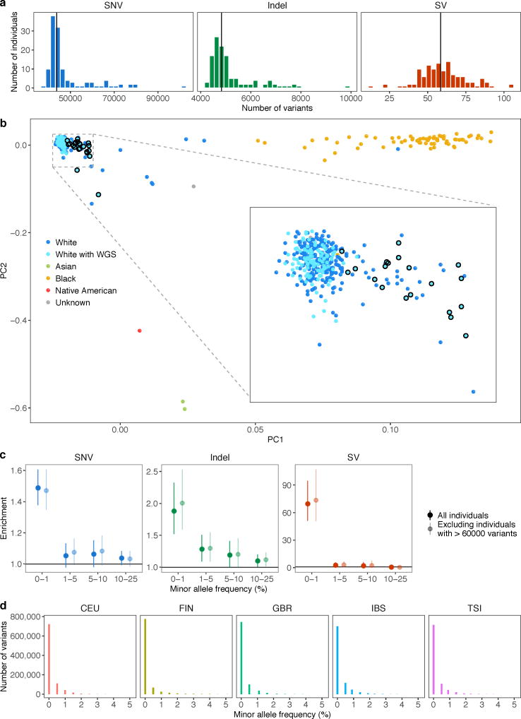
Extended Data Figure 4. Number of rare variants per individual and population structure.

(a) The distribution of the number of rare variants of each type for individuals of European descent (reported as white). Certain individuals harbored many more rare variants than the population median (vertical black line). (b) Principal component analysis of all individuals. Individuals are plotted according to their first two genotype principal components (PCs) and colored by their reported ancestry. White individuals with whole genome sequencing data, included in (a), are colored in a lighter shade of blue and those with 60,000 or more rare variants are circled in black. The individuals with an excess of rare variants likely had African or Asian admixture. (c) Enrichments as in Fig. 2a and excluding individuals with >60,000 rare variants (circled in (b)), which did not substantially affect the enrichment patterns. (d) European population allele frequency distributions in the 1000 Genomes project of rare SNVs and indels analyzed. The rare variants included in our analysis were constrained to have MAF ≤ 0.01 in the 1000 Genomes European super population, but they were also relatively rare in each of the individual European populations.

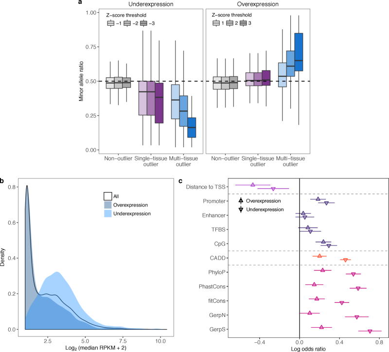
Extended Data Figure 5. Comparison of overexpression and underexpression outliers.

(a) Allele-specific expression (ASE) at rare exonic variants. ASE is shown as the ratio of the number of reads supporting the minor allele to the total number of reads at the site. If the rare variant is driving the extreme expression, we expect this ratio to be below 0.5 for underexpression outliers and above 0.5 for overexpression outliers. Rare coding variants were enriched for ASE in the direction of the extreme expression effect (two-sided Wilcoxon rank sum tests, each nominal P < 4.0 × 10⁻⁸). (b) Expression level distribution of all genes and genes with overexpression or underexpression outliers. Expression is shown as the log₂ of the median (RPKM + 2), where the median was first taken across individuals in each tissue then across expressed tissues for each gene. For genes with low expression, even an RPKM of 0 may not yield a Z-score ≤ −2. Indeed, underexpression outliers were depleted among lowly expressed genes whereas the opposite was true of overexpression outliers (two-sided Wilcoxon rank sum test comparing to all genes, P < 2.2 × 10⁻¹⁶ for both overexpression and underexpression). (c) Feature enrichments (as in Fig. 3b) shown separately for over and underexpression outliers.

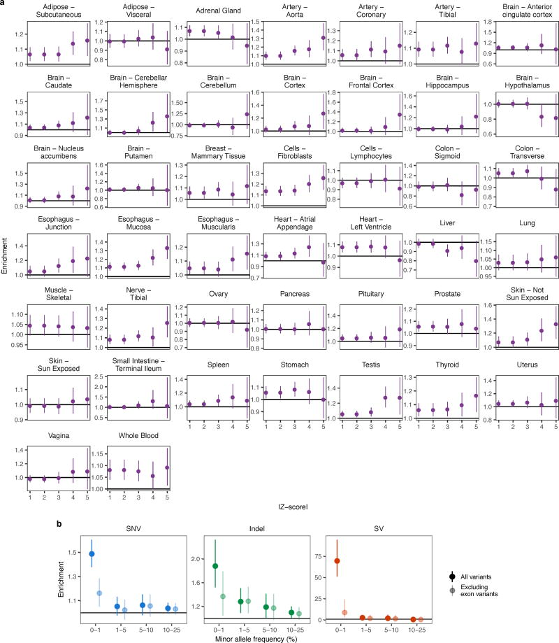
Extended Data Figure 6. Extended rare variant enrichments.

(a) For each tissue, rare SNV enrichment in single-tissue outliers compared with non-outliers at the same genes for increasing Z-score thresholds. Enrichments calculated as in Fig. 2. The rare variant enrichments varied between tissues though the overall pattern mirrored that of multi-tissue outliers when combining all the tissues (Fig. 2b). The high variance in the enrichments underscores the noise in single-tissue outlier discovery. (b) As in Fig. 2a, enrichment for SNVs, indels, and SVs in outliers compared with the same genes in non-outliers either including all rare variants or only those outside protein-coding or lincRNA exons in Gencode v19 annotation. The enrichment of rare variants was weaker, but still significant, for all variant types when excluding exonic regions.

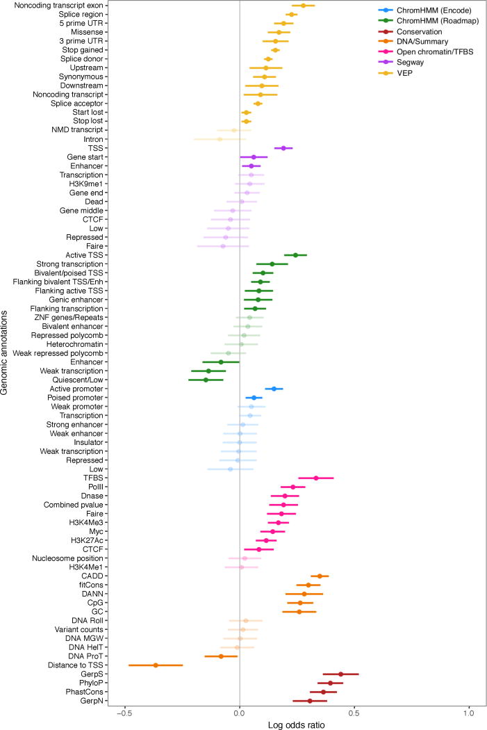
Extended Data Figure 7. Enrichment of an extended list of functional genomic annotations.

Log odds ratios and 95% Wald confidence intervals from logistic regression models of outlier status as a function of each genomic feature. Features were calculated among rare SNVs within 10 kb of the gene. When more than one feature corresponded to the same genomic annotation (e.g., the number or the presence of rare variants in a splice region; Supplementary Table 3b), the feature with the highest enrichment is shown. Lighter shading indicates a non-significant log odds ratio (nominal P > 0.05).

Extended Data Figure 8. Evolutionary constraint and regulatory control of multi-tissue outlier genes.

(a) Odds ratio of being intolerant to synonymous and missense variants for genes with multi-tissue eQTLs (eGenes), genes with multi-tissue outliers, OMIM, and GWAS genes (see Methods). As expected, GWAS and OMIM genes showed no enrichment or depletion for synonymous variation intolerant genes. Genes with multi-tissue outliers and eGenes showed slight depletion for these genes. Genes with multi-tissue outliers and eGenes were strongly depleted for missense variation intolerant genes compared with OMIM and GWAS genes. (b) Comparison of the depletion of disease genes among genes with a multi-tissue outlier and eGenes. Similar to Fig. 4c, bars represent 95% confidence intervals from Fisher’s exact test. (c) For each of ten gene lists, the difference in the mean number of variants near genes in the list compared with the mean for all other annotated genes. Results are stratified by minor allele frequency, and bars indicate the 95% confidence interval for the difference from a two-sided t-test. Disease genes harbored more variants than control genes in general, and the difference was particularly striking for rare variants. This suggests that the depletion of outliers and eQTLs for certain groups of disease genes is due to less rare variation near these genes. Instead, we hypothesize that the variation around these genes in our healthy cohort is less likely to have large regulatory effects. (d) Distribution of the number of tissues with an eQTL for genes with and without outliers. Genes with multi-tissue outliers had eQTLs in more tissues than genes without, which suggests that they are more susceptible to shared regulatory control. This result held for both multi-tissue eQTL definitions (see Methods; Meta-Tissue: 23 vs 3 tissues, Wilcoxon rank sum test P < 2.2 × 10⁻¹⁶; tissue-by-tissue: 7 vs 3 tissues, P < 2.2 × 10⁻¹⁶). (e) This eGene enrichment was robust across different mean expression levels across tissues (two-sided Wilcoxon rank sum tests, Bonferroni-adjusted P < 1 × 10⁻¹¹).

Extended Data Figure 9. River performance.

(a) Comparison between the predictive power of RIVER and that of the genomic annotation model, as in Fig. 5a, across different Z-score thresholds for outlier calling. Increasing the Z-score threshold improved AUC values, but reduced the number of outlier examples, which led to noisy ROCs. (b) Stability analysis of estimated parameters with different parameter initializations (see Methods). (c) Correlations, using Kendall’s tau, between the fraction of tissues with |Z-score| ≥ 2 and the test probabilities from the genomic annotation model (left) and RIVER (right). We calculated test posterior probabilities using 10-fold cross validation and only considered individual and gene pairs with a fraction of tissues with |Z-score| ≥ 2 that was significantly different from 0.05 (one-sided binomial exact test, Benjamini-Hochberg adjusted P < 0.05). (d) P-values from a one-sided Fisher’s exact test measuring the association between allelic imbalance (see Methods) and the posterior probability of a functional rare variant according to the genomic annotation model and RIVER. The posterior probabilities from RIVER were more strongly associated with allelic imbalance across all four thresholds tested. (e) Assessment of the advantage of incorporating gene expression with genomic annotations for predicting outlier status using simplified supervised models (see Methods). All models showed consistent improvement of the log odds ratio of outlier status when incorporating expression. (f) Performance of models with 12 individual genomic features compared with the genomic annotation model and RIVER. Some models with single genomic features provided slightly better AUCs compared with the genomic annotation model, but they were not statistically different. On the other hand, RIVER predicted the effects of rare variants significantly better than each of the models with a single feature.

Extended Data Figure 10. Evaluation of known pathogenic variants using RIVER.

(a) 27 GTEx rare SNVs reported as disease variants in ClinVar. Relative frequency of (b) the |median Z-score|, (c) posterior probabilities from the genomic annotation model, and (d) posterior probabilities from RIVER for all individual and gene pairs (grey) and 27 pairs with pathogenic variants from ClinVar (orange). P-values were computed using a two-sided Wilcoxon rank sum test. We note that rare indels and SVs were not found nearby the genes in the individuals carrying these pathogenic variants. (e and f) Z-score and RPKM distributions for (e) SBDS and (f) GAMT were compared with the values for four individuals carrying regulatory pathogenic variation (red asterisks and triangles). The median Z-score and RPKM values across tissues are shown at the top of each plot (black circle). Tissues are colored as in Fig. 1 and sorted in decreasing order of the difference between the average Z-score of individuals with a regulatory pathogenic variant and the median Z-score for the tissue. Three individuals carrying a total of two unique rare variants are shown for SBDS. Both variants are associated with the recessive Shwachman-Diamond syndrome, which causes systemic symptoms including pancreatic, neurological, and hematologic abnormalities⁴⁶ and can disrupt fibroblast function⁴⁷. The individuals, being heterozygous for these variants, lacked the disease phenotype. Nonetheless, we saw extreme underexpression of SBDS across almost all tissues in these individuals, including brain tissues, fibroblasts, and pancreas. One individual had a rare variant for GAMT associated with cerebral creatine deficiency syndrome 2, shown to cause neurological deficiencies and also lead to low body fat⁴⁸. The individual had the most extreme underexpression in (subcutaneous) adipose.

Extended Data Figure 11. Validation of large-effect rare variants via CRISPR/Cas9 genome editing.

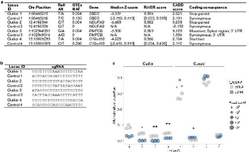
(a) SNVs in outliers and controls assayed for expression effects using CRISPR/Cas9 genome editing. For common SNVs in controls (MAF >1% in the GTEx cohort), the range of median Z-scores and RIVER scores are given for all individuals harboring the minor allele. Missing values indicate that the variant was absent from our cohort. (b) Single-guide RNAs (sgRNAs) for four SNVs found in outliers and four control SNVs in the same genes. (c) Alternate (installed) gDNA and cDNA allele proportions for four rare, coding SNVs in outliers (left) and four matched control SNVs (right). Each gDNA and cDNA sample was sequenced in triplicate (technical replicates). Asterisks denote the Bonferroni-adjusted significance level from a two-sided t-test of the difference between the gDNA and cDNA alternate allele proportions: P < 0.05 (.), P < 0.01 (*), and P < 0.001 (**). Though one control SNV showed a significant difference in the alternate allele proportion between cDNA and gDNA, it displayed an increase rather than a decrease in expression.

Appendix

Laboratory, Data Analysis and Coordinating Center (LDACC) - Analysis Working Group (AWG)

François Aguet¹, Kristin G. Ardlie¹, Beryl B. Cummings^1,2, Ellen T. Gelfand¹, Gad Getz^1,3,4, Kane Hadley¹, Katherine H. Huang¹, Monkol Lek^1,2, Xiao Li¹, Daniel G. MacArthur^1,2, Jared L. Nedzel¹, Duyen T. Nguyen¹, Michael S. Noble¹, Ayellet V. Segrè¹, Casandra A. Trowbridge¹

Funded Statistical Methods groups - Analysis Working Group (AWG)

Nathan S. Abell^5,6, Alexis Battle⁷, Gireesh K. Bogu^8,9, Andrew Brown^10,11,12, Christopher D. Brown¹³, Stephane Castel^14,15, Colby Chiang¹⁶, Don Conrad^17,18, Nancy J. Cox^19,21,25, Farhan N. Damani⁷, Joe R. Davis^5,6, Olivier Delaneau^10,11,12, Emmanouil T. Dermitzakis^10,11,12, Barbara E. Engelhardt²², Eleazar Eskin^23,24, Laure Fresard^5,6, Eric R. Gamazon^19,21,25, Diego Garrido-Martín^8,9, Ariel Gewirtz²⁶, Genna Gliner²⁷, Michael J. Gloudemans^5,6,28, Roderic Guigo^8,9,29, Ira Hall^16,30,17, Buhm Han³¹, Yuan He³², Farhad Hormozdiari²³, Cedric Howald^10,11,12, Hae Kyung Im³³, Brian Jo²⁶, Eun Yong Kang²³, Yungil Kim⁷, Sarah Kim-Hellmuth^14,15, Tuuli Lappalainen^14,15, Xin Li^5,6, Boxiang Liu^5,6,34, Serghei Mangul²³, Mark I. McCarthy^35,36,37, Ian C. McDowell³⁸, Pejman Mohammadi^14,15, Jean Monlong^8,9,39, Stephen B. Montgomery^5,6, Sara Mostafavi⁴⁰, Manuel Muñoz-Aguirre^8,9,41, Anne W. Ndungu³⁵, Dan L. Nicolae^33,42,43, Andrew B. Nobel^44,45, Halit Ongen^10,11,12, John J. Palowitch⁴⁴, Nikolaos Panousis^10,11,12, Panagiotis Papasaikas^9,46, YoSon Park¹³, Princy Parsana⁷, Anthony J. Payne³⁵, Christine Peterson⁴⁷, Jonathan K. Pritchard^5,34,43,48, Ferran Reverter^8,9,49, Chiara Sabatti^50,51, Ashis Saha⁷, Alexandra Scott¹⁶, Andrey A. Shabalin⁵², Reza Sodaei^8,9, Matthew Stephens^42,43, Benjamin J. Strober³², Jae Hoon Sul⁵³, Emily K. Tsang^5,6,28, Sarah Urbut⁴³, Martijn van de Bunt^35,36, Xiaoquan Wen⁵⁴, Fred A. Wright⁵⁵, Zachary Zappala^5,6, Yi-Hui Zhou⁵⁵

enhancing GTEx (eGTEx) funded groups

Joshua Akey⁵⁶, Daniel Bates⁵⁷, Lin Chen⁵⁸, Kathryn Demanelis⁵⁸, Morgan Diegel⁵⁷, Jennifer Doherty⁵⁹, Andrew P. Feinberg^32,60,61,62, Marian Fernando^33,63, Jessica Halow⁵⁷, Kasper D. Hansen^60,64,65, Eric Haugen⁵⁷, Peter Hickey⁶⁵, Farzana Jasmine⁵⁸, Lihua Jiang⁵, Audra Johnson⁵⁷, Rajinder Kaul⁵⁷, Manolis Kellis^1,66, Muhammad G. Kibriya⁵⁸, Kristen Lee⁵⁷, Jin Billy Li⁵, Qin Li5, Shin Lin^5,67, Stephen B. Montgomery^5,6, Meritxell Oliva^33,63, Brandon L. Pierce⁵⁸, Lindsay F. Rizzardi⁶⁰, Richard Sandstrom⁵⁷, Kevin S. Smith^5,6, Michael Snyder⁵, John Stamatoyannopoulos⁵⁷, Barbara E. Stranger^33,63,68, Hua Tang⁵, Emily K. Tsang^5,6,28, Rui Zhang⁵

NIH Common Fund

Concepcion R. Nierras⁶⁹

NIH/NCI

Philip A. Branton⁷⁰, Latarsha J. Carithers⁷¹, Ping Guan⁷⁰, Helen M. Moore⁷⁰, Abhi Rao⁷⁰, Jimmie B. Vaught⁷⁰,

NIH/NHGRI

Lockhart C. Nicole⁷², Jeffery P. Struewing⁷², Simona Volpi⁷²

NIH/NIMH

Anjene M. Addington⁷³, Susan E. Koester⁷³

NIH/NIDA

A. Roger Little⁷⁴

Biospecimen Collection Source Site - NDRI

Lori E. Brigham⁷⁵, Richard Hasz⁷⁶, Marcus Hunter⁷⁷, Christopher Johns⁷⁸, Mark Johnson⁷⁹, Gene Kopen⁸⁰, William F. Leinweber⁸⁰, John T. Lonsdale⁸⁰, Alisa McDonald⁸⁰, Bernadette Mestichelli⁸⁰, Kevin Myer⁷⁷, Brian Roe⁷⁷, Michael Salvatore⁸⁰, Saboor Shad⁸⁰, Jeffrey A. Thomas⁸⁰, Gary Walters⁷⁹, Michael Washington⁷⁹, Joseph Wheeler⁷⁸

Biospecimen Collection Source Site - RPCI

Jason Bridge⁸¹, Barbara A. Foster⁸², Bryan M. Gillard⁸², Ellen Karasik⁸², Rachna Kumar⁸², Mark Miklos⁸¹, Michael T. Moser⁸²

Biospecimen Core Resource - VARI

Scott D. Jewell⁸³, Robert G. Montroy⁸³, Daniel C. Rohrer⁸³, Dana Valley⁸³

Brain Bank Repository - U Miami

David A. Davis⁸⁴, Deborah C. Mash⁸⁴

Leidos Biomedical - Project Management

Anita H. Undale⁸⁵, Anna M. Smith⁸⁶, David E. Tabor⁸⁶, Nancy V. Roche⁸⁶, Jeffrey A. McLean⁸⁶, Negin Vatanian⁸⁶, Karna L. Robinson⁸⁶, Leslie Sobin⁸⁶, Mary E. Barcus⁸⁷, Kimberly M. Valentino⁸⁶, Liqun Qi⁸⁶, Stephen Hunter⁸⁶, Pushpa Hariharan⁸⁶, Shilpi Singh⁸⁶, Ki Sung Um⁸⁶, Takunda Matose⁸⁶, Maria M. Tomadzewski⁸⁶

ELSI Study

Laura K. Barker⁸⁸, Maghboeba Mosavel⁸⁹, Laura A. Siminoff⁸⁸, Heather M. Traino⁸⁸

Genome Browser Data Integration, and Visualization - EBI

Paul Flicek⁹⁰, Thomas Juettmann⁹⁰, Magali Ruffier⁹⁰, Dan Sheppard⁹⁰, Kieron Taylor⁹⁰, Steven Trevanion⁹⁰, Daniel R. Zerbino⁹⁰

Genome Browser Data Integration, and visualization - UCSC Genomics Institute, University of California Santa Cruz

Brian Craft⁹¹, Mary Goldman⁹¹, Maximilian Haeussler⁹¹, W. James Kent⁹¹, Christopher M. Lee⁹¹, Benedict Paten⁹¹, Kate R. Rosenbloom⁹¹, John Vivan⁹¹, Jingchun Zhu⁹¹

Unfunded members of the Analysis Working Group (AWG)

Ruth Barshir⁹², Omer Basha⁹², Pedro G. Ferreira^93,94, Gen Li⁹⁵, Matthew T. Maurano⁹⁶, Jie Quan⁹⁷, Michael Sammeth⁹⁸, Hualin S. Xi⁹⁷, Esti Yeger-Lotem^92,99, Judith B. Zaugg¹⁰⁰

¹The Broad Institute of Massachusetts Institute of Technology and Harvard University, Cambridge, MA 02142, USA. ²Analytic and Translational Genetics Unit, Massachusetts General Hospital, Boston, MA 02114, USA. ³Massachusetts General Hospital Cancer Center, Massachusetts General Hospital, Boston, MA 02114, USA. ⁴Department of Pathology, Harvard Medical School, Boston, MA 02114, USA. ⁵Department of Genetics, Stanford University, Stanford, CA 94305, USA. ⁶Department of Pathology, Stanford University, Stanford, CA 94305, USA. ⁷Department of Computer Science, Johns Hopkins University, Baltimore, MD 21218, USA. ⁸Centre for Genomic Regulation (CRG), The Barcelona Institute for Science and Technology, 08003 Barcelona, Spain. ⁹Universitat Pompeu Fabra, 08003 Barcelona, Catalonia, Spain. ¹⁰Department of Genetic Medicine and Development, University of Geneva Medical School, 1211 Geneva, Switzerland. ¹¹Institute for Genetics and Genomics in Geneva (iG3), University of Geneva, 1211 Geneva, Switzerland. ¹²Swiss Institute of Bioinformatics, 1211 Geneva, Switzerland. ¹³Department of Genetics, Perelman School of Medicine, University of Pennsylvania, Philadelphia, PA 19104, USA. ¹⁴New York Genome Center, New York, NY 10013, USA. ¹⁵Department of Systems Biology, Columbia University Medical Center, New York, NY 10032, USA. ¹⁶McDonnell Genome Institute, Washington University School of Medicine, St. Louis, MO 63108, USA. ¹⁷Department of Genetics, Washington University School of Medicine, St. Louis, MO 63108, USA. ¹⁸Department of Pathology & Immunology, Washington University School of Medicine, St. Louis, MO 63108, USA. ¹⁹Division of Genetic Medicine, Department of Medicine, Vanderbilt University Medical Canter, Nashville, TN 37232, USA. ²⁰Department of Clinical Epidemiology, Biostatistics and Bioinformatics, University of Amsterdam, 1105 AZ Amsterdam, The Netherlands. ²¹Department of Psychiatry, Academic Medical Center, University of Amsterdam, 1105 AZ Amsterdam, The Netherlands. ²²Center for Statistics and Machine Learning, Department of Computer Science, Princeton University, Princeton, NJ 08540, USA. ²³Department of Computer Science, University of California, Los Angeles, CA 90095, USA. ²⁴Department of Human Genetics, University of California, Los Angeles, CA 90095, USA. ²⁵Department of Clinical Epidemiology, Biostatistics and Bioinformatics, Academic Medical Center, University of Amsterdam, 1105 AZ Amsterdam, The Netherlands. ²⁶Lewis Sigler Institute, Princeton University, Princeton, NJ 08540, USA. ²⁷Department of Operations Research and Financial Engineering, Princeton University, Princeton, NJ 08540, USA. ²⁸Biomedical Informatics Program, Stanford University, Stanford, CA 94305, USA. ²⁹Institut Hospital del Mar d'Investigacions Mèdiques (IMIM), 08003 Barcelona, Spain. ³⁰Department of Medicine, Washington University School of Medicine, St. Louis, MO 63108, USA. ³¹Department of Convergence Medicine, University of Ulsan College of Medicine, Asan Medical Center, Korea. ³²Department of Biomedical Engineering, Johns Hopkins University, Baltimore, MD 21218, USA. ³³Section of Genetic Medicine, Department of Medicine, The University of Chicago, Chicago, IL 60637, USA. ³⁴Department of Biology, Stanford University, Stanford, CA 94305, USA. ³⁵Wellcome Trust Centre for Human Genetics Research, Nuffield Department of Clinical Medicine, University of Oxford, Oxford, OX3 7BN, UK. ³⁶Oxford Centre for Diabetes, Endocrinology and Metabolism, University of Oxford, Churchill Hospital, Oxford, OX3 7LE, UK. ³⁷Oxford NIHR Biomedical Research Centre, Churchill Hospital, Oxford, OX3 7LJ, UK. ³⁸Computational Biology & Bioinformatics Graduate Program, Duke University, Durham, NC 27708, USA. ³⁹Human Genetics Department, McGill University, Montreal, Quebec H3A 0G1, Canada. ⁴⁰Department of Computer Science, Stanford University, Stanford, CA 94305, USA. ⁴¹Departament d'Estadística i Investigació Operativa, Universitat Politècnica de Catalunya, 08034 Barcelona, Spain. ⁴²Department of Statistics, The University of Chicago, Chicago, IL 60637, USA. ⁴³Department of Human Genetics, The University of Chicago, Chicago, IL 60637, USA. ⁴⁴Department of Statistics and Operations Research, University of North Carolina, Chapel Hill, NC 27599, USA. ⁴⁵Department of Biostatistics, University of North Carolina, Chapel Hill, NC 27599, USA. ⁴⁶Center for Genomic Regulation (CRG), 08003 Barcelona, Catalonia, Spain. ⁴⁷Department of Biostatistics, The University of Texas MD Anderson Cancer Center, 1400 Pressler Street, Houston, TX 77030, USA. ⁴⁸Howard Hughes Medical Institute. ⁴⁹Universitat de Barcelona, 08028 Barcelona, Catalonia, Spain. ⁵⁰Department of Biomedical Data Science, Stanford Univeristy, Stanford, CA 94305, USA. ⁵¹Department of Statistics, Stanford University, Stanford, CA 94305, USA. ⁵²Center for Biomarker Research and Personalized Medicine, Virginia Commonwealth University, Richmond, VA 23298, USA. ⁵³Department of Psychiatry and Biobehavioral Sciences, University of California, Los Angeles, CA 90095, USA. ⁵⁴Department of Biostatistics, University of Michigan, Ann Arbor, MI 48109, USA. ⁵⁵Bioinformatics Research Center and Departments of Statistics and Biological Sciences, North Carolina State University, Raleigh, NC 27695, USA. ⁵⁶Department of Genome Sciences, University of Washington, Seattle, WA 98195, USA. ⁵⁷Altius Institute for Biomedical Sciences, Seattle, WA 98121, USA. ⁵⁸Department of Public Health Sciences, The University of Chicago, Chicago, IL 60637, USA. ⁵⁹Department of Epidemiology, The Geisel School of Medicine at Dartmouth, Lebanon, NH 03756, USA. ⁶⁰Center for Epigenetics, Johns Hopkins University School of Medicine, Baltimore, MD 21205, USA. ⁶¹Department of Medicine, Johns Hopkins University School of Medicine, Baltimore, MD 21205, USA. ⁶²Department of Mental Health, Johns Hopkins University School of Public Health, Baltimore, MD 21205, USA. ⁶³Institute for Genomics and Systems Biology, The University of Chicago, Chicago, IL 60637, USA. ⁶⁴McKusick-Nathans Institute of Genetic Medicine, Johns Hopkins School of Medicine, Baltimore, MD 21205, USA. ⁶⁵Department of Biostatistics, Johns Hopkins University, Baltimore, MD 21205, USA. ⁶⁶Computer Science and Artificial Intelligence Laboratory, Massachusetts Institute of Technology, Cambridge, MA 02139, USA. ⁶⁷Division of Cardiology, University of Washington, Seattle, WA 98195, USA. ⁶⁸Center for Data Intensive Science, The University of Chicago, Chicago, IL 60637, USA. ⁶⁹Office of Strategic Coordination, Division of Program Coordination, Planning and Strategic Initiatives, Office of the Director, NIH, Rockville, MD 20852, USA. ⁷⁰Biorepositories and Biospecimen Research Branch, Division of Cancer Treatment and Diagnosis, National Cancer Institute, Bethesda, MD 20892, USA. ⁷¹National Institute of Dental and Craniofacial Research, Bethesda, MD 20892, USA. ⁷²Division of Genomic Medicine, National Human Genome Research Institute, Rockville, MD 20852, USA. ⁷³Division of Neuroscience and Basic Behavioral Science, National Institute of Mental Health, NIH, Bethesda, MD 20892, USA. ⁷⁴National Institute on Drug Abuse, NIH, Bethesda, MD 20892, USA. ⁷⁵Washington Regional Transplant Community, Annandale, VA 22003, USA. ⁷⁶Gift of Life Donor Program, Philadelphia, PA 19103, USA. ⁷⁷LifeGift, Houston, TX 77055, USA. ⁷⁸Center for Organ Recovery and Education, Pittsburgh, PA 15238, USA. ⁷⁹LifeNet Health, Virginia Beach, VA 23453, USA. ⁸⁰National Disease Research Interchange, Philadelphia, PA 19103, USA. ⁸¹Unyts, Buffalo, NY 14203, USA. ⁸²Pharmacology and Therapeutics, Roswell Park Cancer Institute, Buffalo, NY 14263, USA. ⁸³Van Andel Research Institute, Grand Rapids, MI 49503, USA. ⁸⁴Brain Endowment Bank, Miller School of Medicine, University of Miami, Miami, FL 33136, USA. ⁸⁵National Institute of Allergy and Infectious Diseases, NIH, Rockville, MD 20852, USA. ⁸⁶Biospecimen Research Group, Clinical Research Directorate, Leidos Biomedical Research, Inc., Rockville, MD 20852, USA. ⁸⁷Leidos Biomedical Research, Inc., Frederick, MD 21701, USA. ⁸⁸Temple University, Philadelphia, PA 19122, USA. ⁸⁹Department of Health Behavior and Policy, School of Medicine, Virginia Commonwealth University, Richmond, VA 23298, USA. ⁹⁰European Molecular Biology Laboratory, European Bioinformatics Institute, Cambridge CB10 1SD, UK. ⁹¹UCSC Genomics Institute, University of California Santa Cruz, Santa Cruz, CA 95064, USA. ⁹²Department of Clinical Biochemistry and Pharmacology, Faculty of Health Sciences, Ben-Gurion University of the Negev, Beer-Sheva 84105, Israel. ⁹³Instituto de Investigação e Inovação em Saúde (i3S), Universidade do Porto, 4200-135 Porto, Portugal. ⁹⁴Institute of Molecular Pathology and Immunology (IPATIMUP), University of Porto, 4200-625 Porto, Portugal. ⁹⁵Department of Biostatistics, Mailman School of Public Health, Columbia University, New York, NY 10032, USA. ⁹⁶Institute for Systems Genetics, New York University Langone Medical Center, New York, New York 10016, USA. ⁹⁷Computational Sciences, Pfizer Inc, Cambridge, MA 02140, USA. ⁹⁸Institute of Biophysics Carlos Chagas Filho (IBCCF), Federal University of Rio de Janeiro (UFRJ), 21941902 Rio de Janeiro, Brazil. ⁹⁹National Institute for Biotechnology in the Negev, Beer-Sheva, 84105 Israel ¹⁰⁰European Molecular Biology Laboratorium, 69117 Heidelberg, Germany.

References

- 1.Tennessen JA, et al. Evolution and functional impact of rare coding variation from deep sequencing of human exomes. Science. 2012;337:64–9. doi: 10.1126/science.1219240. [DOI] [PMC free article] [PubMed] [Google Scholar]
- 2.Nelson MR, et al. An abundance of rare functional variants in 202 drug target genes sequenced in 14,002 people. Science. 2012;337:100–4. doi: 10.1126/science.1217876. [DOI] [PMC free article] [PubMed] [Google Scholar]
- 3.The UK10K Consortium. The UK10K project identifies rare variants in health and disease. Nature. 2015;526:82–90. doi: 10.1038/nature14962. [DOI] [PMC free article] [PubMed] [Google Scholar]
- 4.Keinan A, Clark AG. Recent explosive human population growth has resulted in an excess of rare genetic variants. Science. 2012;336:740–3. doi: 10.1126/science.1217283. [DOI] [PMC free article] [PubMed] [Google Scholar]
- 5.Uricchio LH, Zaitlen NA, Ye CJ, Witte JS, Hernandez RD. Selection and explosive growth alter genetic architecture and hamper the detection of causal rare variants. Genome Res. 2016;26:863–73. doi: 10.1101/gr.202440.115. [DOI] [PMC free article] [PubMed] [Google Scholar]
- 6.MacArthur DG, et al. A systematic survey of loss-of-function variants in human protein-coding genes. Science. 2012;335:823–8. doi: 10.1126/science.1215040. [DOI] [PMC free article] [PubMed] [Google Scholar]
- 7.Narasimhan VM, et al. Health and population effects of rare gene knockouts in adult humans with related parents. Science. 2016;352:474–7. doi: 10.1126/science.aac8624. [DOI] [PMC free article] [PubMed] [Google Scholar]
- 8.Montgomery SB, Lappalainen T, Gutierrez-Arcelus M, Dermitzakis ET. Rare and common regulatory variation in population-scale sequenced human genomes. PLoS Genet. 2011;7 doi: 10.1371/journal.pgen.1002144. [DOI] [PMC free article] [PubMed] [Google Scholar]
- 9.Zhao J, et al. A burden of rare variants associated with extremes of gene expression in human peripheral blood. Am. J. Hum. Genet. 2016;98:299–309. doi: 10.1016/j.ajhg.2015.12.023. [DOI] [PMC free article] [PubMed] [Google Scholar]
- 10.Zeng Y, et al. Aberrant gene expression in humans. PLoS Genet. 2015;11:e1004942. doi: 10.1371/journal.pgen.1004942. [DOI] [PMC free article] [PubMed] [Google Scholar]
- 11.Li X, et al. Transcriptome sequencing of a large human family identifies the impact of rare noncoding variants. Am. J. Hum. Genet. 2014;95:245–56. doi: 10.1016/j.ajhg.2014.08.004. [DOI] [PMC free article] [PubMed] [Google Scholar]
- 12.Main GTEx mansucript, co-submitted.
- 13.Stegle O, Parts L, Piipari M, Winn J, Durbin R. Using probabilistic estimation of expression residuals (PEER) to obtain increased power and interpretability of gene expression analyses. Nat. Protoc. 2012;7:500–7. doi: 10.1038/nprot.2011.457. [DOI] [PMC free article] [PubMed] [Google Scholar]
- 14.Chiang C, et al. The impact of structural variation on human gene expression. Nat. Genet. 2017 doi: 10.1038/ng.3834. [DOI] [PMC free article] [PubMed] [Google Scholar]
- 15.Pollard KS, Hubisz MJ, Rosenbloom KR, Siepel A. Detection of nonneutral substitution rates on mammalian phylogenies. Genome Res. 2010;20:110–21. doi: 10.1101/gr.097857.109. [DOI] [PMC free article] [PubMed] [Google Scholar]
- 16.Siepel A, et al. Evolutionarily conserved elements in vertebrate, insect, worm, and yeast genomes. Genome Res. 2005;15:1034–50. doi: 10.1101/gr.3715005. [DOI] [PMC free article] [PubMed] [Google Scholar]
- 17.Cooper GM, et al. Distribution and intensity of constraint in mammalian genomic sequence. Genome Res. 2005;15:901–13. doi: 10.1101/gr.3577405. [DOI] [PMC free article] [PubMed] [Google Scholar]
- 18.Arbiza L, et al. Genome-wide inference of natural selection on human transcription factor binding sites. Nat. Genet. 2013;45:723–9. doi: 10.1038/ng.2658. [DOI] [PMC free article] [PubMed] [Google Scholar]
- 19.Kircher M, et al. A general framework for estimating the relative pathogenicity of human genetic variants. Nat. Genet. 2014;46:310–5. doi: 10.1038/ng.2892. [DOI] [PMC free article] [PubMed] [Google Scholar]
- 20.Green RC, et al. ACMG recommendations for reporting of incidental findings in clinical exome and genome sequencing. Genet. Med. 2013;15:565–74. doi: 10.1038/gim.2013.73. [DOI] [PMC free article] [PubMed] [Google Scholar]
- 21.Landrum MJ, et al. ClinVar: public archive of interpretations of clinically relevant variants. Nucleic Acids Res. 2016;44:D862–8. doi: 10.1093/nar/gkv1222. [DOI] [PMC free article] [PubMed] [Google Scholar]
- 22.Hendel A, et al. Chemically modified guide RNAs enhance CRISPR-Cas genome editing in human primary cells. Nat. Biotechnol. 2015;33:985–9. doi: 10.1038/nbt.3290. [DOI] [PMC free article] [PubMed] [Google Scholar]
- 23.Hess GT, et al. Directed evolution using dCas9-targeted somatic hypermutation in mammalian cells. Nat. Methods. 2016;13:1036–1042. doi: 10.1038/nmeth.4038. [DOI] [PMC free article] [PubMed] [Google Scholar]
- 24.Grundberg E, et al. Global analysis of DNA methylation variation in adipose tissue from twins reveals links to disease-associated variants in distal regulatory elements. Am. J. Hum. Genet. 2013;93:876–90. doi: 10.1016/j.ajhg.2013.10.004. [DOI] [PMC free article] [PubMed] [Google Scholar]
- 25.Gamazon ER, et al. Enrichment of cis-regulatory gene expression SNPs and methylation quantitative trait loci among bipolar disorder susceptibility variants. Mol. Psychiatry. 2013;18:340–6. doi: 10.1038/mp.2011.174. [DOI] [PMC free article] [PubMed] [Google Scholar]
- 26.Bell JT, et al. DNA methylation patterns associate with genetic and gene expression variation in HapMap cell lines. Genome Biol. 2011;12:R10. doi: 10.1186/gb-2011-12-1-r10. [DOI] [PMC free article] [PubMed] [Google Scholar]
- 27.Waszak SM, et al. Population variation and genetic control of modular chromatin architecture in humans. Cell. 2015;162:1039–50. doi: 10.1016/j.cell.2015.08.001. [DOI] [PubMed] [Google Scholar]
- 28.Grubert F, et al. Genetic control of chromatin states in humans involves local and distal chromosomal interactions. Cell. 2015;162:1051–65. doi: 10.1016/j.cell.2015.07.048. [DOI] [PMC free article] [PubMed] [Google Scholar]
- 29.DeLong ER, DeLong DM, Clarke-Pearson DL. Comparing the areas under two or more correlated receiver operating characteristic curves: a nonparametric approach. Biometrics. 1988;44:837–45. [PubMed] [Google Scholar]
- 30.1000 Genomes Project Consortium. A global reference for human genetic variation. Nature. 2015;526:68–74. doi: 10.1038/nature15393. [DOI] [PMC free article] [PubMed] [Google Scholar]
- 31.The Roadmap Epigenomics Consortium. Integrative analysis of 111 reference human epigenomes. Nature. 2015;518:317–30. doi: 10.1038/nature14248. [DOI] [PMC free article] [PubMed] [Google Scholar]
- 32.McLaren W, et al. The Ensembl Variant Effect Predictor. Genome Biol. 2016;17:122. doi: 10.1186/s13059-016-0974-4. [DOI] [PMC free article] [PubMed] [Google Scholar]
- 33.Panousis NI, Gutierrez-Arcelus M, Dermitzakis ET, Lappalainen T. Allelic mapping bias in RNA-sequencing is not a major confounder in eQTL studies. Genome Biol. 2014;15:467. doi: 10.1186/s13059-014-0467-2. [DOI] [PMC free article] [PubMed] [Google Scholar]
- 34.Sul JH, Han B, Ye C, Choi T, Eskin E. Effectively identifying eQTLs from multiple tissues by combining mixed model and meta-analytic approaches. PLoS Genet. 2013;9:e1003491. doi: 10.1371/journal.pgen.1003491. [DOI] [PMC free article] [PubMed] [Google Scholar]
- 35.Lek M, et al. Analysis of protein-coding genetic variation in 60,706 humans. Nature. 2016;536:285–291. doi: 10.1038/nature19057. [DOI] [PMC free article] [PubMed] [Google Scholar]
- 36.Welter D, et al. The NHGRI GWAS Catalog, a curated resource of SNP-trait associations. Nucleic Acids Res. 2014;42:D1001–6. doi: 10.1093/nar/gkt1229. [DOI] [PMC free article] [PubMed] [Google Scholar]
- 37.Deciphering Developmental Disorders Study. Large-scale discovery of novel genetic causes of developmental disorders. Nature. 2015;519:223–8. doi: 10.1038/nature14135. [DOI] [PMC free article] [PubMed] [Google Scholar]
- 38.Dempster A, Laird N, Rubin D. Maximum Likelihood from incomplete data via the EM algorithm. J. R. Stat. Soc. 1977;39:1–38. [Google Scholar]
- 39.Adzhubei IA, et al. A method and server for predicting damaging missense mutations. Nat. Methods. 2010;7:248–9. doi: 10.1038/nmeth0410-248. [DOI] [PMC free article] [PubMed] [Google Scholar]
- 40.Ng PC, Henikoff S. Predicting deleterious amino acid substitutions. Genome Res. 2001;11:863–74. doi: 10.1101/gr.176601. [DOI] [PMC free article] [PubMed] [Google Scholar]
- 41.Quang D, Chen Y, Xie X. DANN: a deep learning approach for annotating the pathogenicity of genetic variants. Bioinformatics. 2015;31:761–3. doi: 10.1093/bioinformatics/btu703. [DOI] [PMC free article] [PubMed] [Google Scholar]
- 42.ENCODE Project Consortium. An integrated encyclopedia of DNA elements in the human genome. Nature. 2012;489:57–74. doi: 10.1038/nature11247. [DOI] [PMC free article] [PubMed] [Google Scholar]
- 43.Martin M. Cutadapt removes adapter sequences from high-throughput sequencing reads. EMBnet.journal. 2011;17:10. [Google Scholar]
- 44.Li H, Durbin R. Fast and accurate short read alignment with Burrows-Wheeler transform. Bioinformatics. 2009;25:1754–60. doi: 10.1093/bioinformatics/btp324. [DOI] [PMC free article] [PubMed] [Google Scholar]
- 45.Morgan M, Pagès H, Obenchain V, Hayden N. Rsamtools: Binary alignment (BAM), FASTA, variant call (BCF), and tabix file import [Google Scholar]
- 46.Dror Y, Freedman MH. Shwachman-diamond syndrome. Br. J. Haematol. 2002;118:701–13. doi: 10.1046/j.1365-2141.2002.03585.x. [DOI] [PubMed] [Google Scholar]
- 47.Austin KM, et al. Mitotic spindle destabilization and genomic instability in Shwachman-Diamond syndrome. J. Clin. Invest. 2008;118:1511–8. doi: 10.1172/JCI33764. [DOI] [PMC free article] [PubMed] [Google Scholar]
- 48.Schmidt A, et al. Severely altered guanidino compound levels, disturbed body weight homeostasis and impaired fertility in a mouse model of guanidinoacetate N-methyltransferase (GAMT) deficiency. Hum. Mol. Genet. 2004;13:905–21. doi: 10.1093/hmg/ddh112. [DOI] [PubMed] [Google Scholar]
Associated Data
This section collects any data citations, data availability statements, or supplementary materials included in this article.
Supplementary Materials
Data Availability Statement