Conductivity tensor mapping of the human brain using diffusion tensor MRI

Abstract

Knowledge of the electrical conductivity properties of excitable tissues is essential for relating the electromagnetic fields generated by the tissue to the underlying electrophysiological currents. Efforts to characterize these endogenous currents from measurements of the associated electromagnetic fields would significantly benefit from the ability to measure the electrical conductivity properties of the tissue noninvasively. Here, using an effective medium approach, we show how the electrical conductivity tensor of tissue can be quantitatively inferred from the water self-diffusion tensor as measured by diffusion tensor magnetic resonance imaging. The effective medium model indicates a strong linear relationship between the conductivity and diffusion tensor eigenvalues (respectively, σ and d) in agreement with theoretical bounds and experimental measurements presented here (σ/d ≈ 0.844 ± 0.0545 S⋅s/mm³, r² = 0.945). The extension to other biological transport phenomena is also discussed.

Excitable tissues such as nerve and muscle mediate communication through electrical currents. These endogenous currents are capable of generating electromagnetic fields sufficiently large to be measured outside of the body by using, for example, electro/magnetoencephalography (EEG/MEG) in the case of the brain or electro/magnetocardiography (ECG/MCG) for the heart (1). The three-dimensional spatial distribution of the underlying currents can be estimated from the measured electromagnetic fields through a model-based inversion procedure that, in combination with the measuring method, is referred to as electromagnetic source imaging (ESI).

The modeling component in ESI, the so-called forward model, requires solving the quasistatic Maxwell equations in a resistor model of the anatomical region of interest—for example, the head or sternum. The underlying current distribution can then be estimated by analytical or numerical inversion of the forward model. This method has been employed to localize the electrophysiological generators associated with cardiac and neural activity in various states of health and disease, but the accuracy of the reconstructions depends sensitively on the accuracy of the conductivity values assumed for the tissue. Modeling studies have shown, for example, that the external electromagnetic fields, specifically the local field potentials measured by electroencephalography/cardiography (and, to a lesser extent, the magnetic field recorded by magnetoencephalography/cardiography), are highly sensitive to the electrical conductivity inhomogeneity and anisotropy of tissue (2–7). Hence, the lack of knowledge regarding the true electrical conductivity of the tissue can result in significant mischaracterization of the underlying currents.

Efforts to develop an imaging modality to quantitatively measure the electrical conductivity of tissue noninvasively have largely been thwarted by anatomical and biophysical barriers: the organ of interest can be shielded by highly resistive barriers such as the bony tissue of the skull, and the tissue can exhibit significant reactance, anisotropy, and microstructural heterogeneity. The difficulties associated with imaging biological conductivity in vivo can be appreciated by considering the limitations of electrical impedance tomography (8): the technique exhibits poor spatial resolution past resistive interfaces, particularly at the low frequencies of physiological interest; contains an ill-posed inverse problem; and requires delivering current to the tissue. Other methods suffer from additional shortcomings: magnetic resonance Hall effect imaging (9) relies on propagation of ultrasound into the tissue, and is not quantitative; and magnetic resonance current density imaging requires applying external currents sufficiently large to produce magnetic field contrast visible by MRI (10).

We have previously proposed that the electrical conductivity tensor of tissue can be quantitatively inferred from the water self-diffusion tensor as measured by diffusion tensor magnetic resonance imaging (DTI) (12, 13).‖ DTI employs an pulsed-gradient spin echo to measure the self-diffusion tensor of water in the tissue (13). The hypothesized relationship between electrical conductivity and water self-diffusion in tissue is prompted by the observation that, although there is no fundamental relationship between the two transport modes in free solution, in a structured medium such as tissue the two processes are related through mutual respect for the boundary conditions imposed by the tissue geometry. The possibility of a connection between the conductivity and diffusion tensors can be further motivated by reports that the two tensors exhibit comparable anisotropy (on the order of ten) in cerebral white matter (14, 15).

Connections between phenomenologically distinct transport processes, so-called “cross-property” relations, have been derived, either exactly or in the form of bounds, for a broad range of transport and mechanical properties (16–18) of porous media, yet the framework has not been applied widely to biological tissues. Previously, we have studied the conductivity–diffusion cross-property in brain tissue by using Monte Carlo simulations and a self-consistent effective medium approximation (12, 19),‖ but an exact formulation remained open. Here, using an effective medium framework, we derive a rigorous relationship between the conductivity and diffusion tensors without the need for any assumptions on the tissue geometry, and employing a few limited assumptions on the cell membrane properties. Significantly, the model indicates a strong linear relationship between the conductivity and diffusion tensor eigenvalues, in agreement with theoretical bounds and experimental measurements reported here.

Model

The relationship between a general transport tensor—for example, the conductivity or diffusion tensor—and the underlying microstructure of the medium can be obtained from a perturbation expansion in the statistical correlations of the microstructure. Originally developed by Brown for two-phase isotropic media (20, 21) and later extended to two-phase anisotropic media by Sen and Torquato (22), the statistical correlation expansion, also referred to as a contrast moment expansion, provides a framework for relating distinct transport tensors through the statistics of the medium microstructure. The two-phase model consisting of an inclusion phase embedded in a host phase is particularly amenable to describing biological tissues because the extracellular space can be taken as the host phase and the intracellular space as the inclusion phase.

To derive the cross-property relation between the conductivity and diffusion tensors in brain tissue, the approach we adopt here is to estimate the statistical moments of the microstructure from the observed diffusion tensor, and then derive the conductivity tensor from the estimated moments. We assume in the following that the cell membrane is freely permeable to water and impermeable to charge-carriers on the experimental time scale (≈50 ms). Following Sen and Torquato (22), the effective transport tensor Λ, denoting either the effective electrical conductivity tensor σ or the diffusion tensor D, for a two-phase anisotropic medium of arbitrary topology is given by

1

where φ_i is the inclusion (intracellular) volume fraction, U is the identity tensor, and λ_i and λ_e are, respectively, the inclusion (intracellular) and host medium (extracellular) transport coefficients; for example, in the case of diffusion d_i is the intracellular diffusion coefficient and d_e is the extracellular diffusion coefficient. Similarly, σ_i is the intracellular conductivity value and σ_e is the extracellular conductivity. The dimensionless contrast factors β and B are defined as

2

and

3

The rank-2 tensors A contain the microstructure information and are defined as integrals over the n-point probability functions S, which give the probability of finding n points within the inclusion (intracellular) phase. Exact expressions for A are available in ref. 22.

By setting A = −φ_iU, the first term on the right-hand side of Eq. 1 can be embedded in the sum to give

4

where we have defined β_λ = β(λ_i, λ_e). The sum in the right-hand side of the above equation can be made implicit by defining the concatenation C⁽ⁱ⁾ = (A|A|…), and, similarly, G_λ = (β_λU|βU|…)^T. Eq. 4 then becomes

5

We can obtain a least-squares estimate Ĉ⁽ⁱ⁾ for C⁽ⁱ⁾ based on the observed diffusion tensor D by identifying Λ with D in Eq. 5 and then multiplying from the right by the right-handed Moore–Penrose pseudoinverse G = G(G_dG)⁻¹** yielding

6

Identifying Λ in Eq. 5 with σ and equating Ĉ⁽ⁱ⁾ and C⁽ⁱ⁾ gives

7

Solving algebraically for GG_σ we obtain

8

Finally, solving for σ yields

9

where

10

The two equations above relate the conductivity and diffusion tensors solely in terms of the intra- and extracellular transport coefficients, independently of the microstructural statistics A and the cell volume fraction φ_i. We also observe that the above relationship implies that the conductivity and diffusion tensors share the same eigenvectors. Note that we have not made any assumptions yet on the type of transport tensors involved so that Eq. 10 applies generally to the broader class of transport tensors including hydraulic permeability, acoustic conductivity, etc.

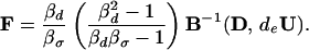
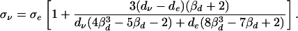
The equivalence between the conductivity and diffusion tensor eigenvectors allows us to express the cross-property relation solely in terms of the conductivity and diffusion tensor eigenvalues, respectively, σ_ν, and d_ν, which we do in the following. The cross-property relation can be simplified by noting that at the quasistatic frequencies of physiological interest (<1 kHz) (23) the intracellular space is effectively shielded by the high resistivity of the cell membrane. The intracellular conductivity can therefore be taken as negligible. Substituting σ_i = 0 into Eqs. 9 and 10 gives

11

The above equation indicates a fractional linear relationship between the conductivity and diffusion tensor eigenvalues. The relationship is highly linear, however, because d_e(8β − 7β_d + 2) will tend to be much larger than d_ν(4β − 5β_d − 2), particularly for small intracellular diffusion values. We can obtain an explicit linear approximation to Eq. 11 by taking a series expansion in the intracellular diffusion

12

Note that both the linear approximation (Eq. 12) and the exact fractional linear relationship given by Eq. 11 satisfy the necessary conditions σ_ν ∝ σ_e and σ_ν/σ_e → d_ν/d_e as d_i → 0, with the latter limit providing the upper-bound σ_ν/σ_e ≤ d_ν/d_e. For the sake of interest, this bound can be compared to the Milton bound between the bulk elastic modulus K and conductivity K/K_e ≤ σ/σ_e of an isotropic material (24).

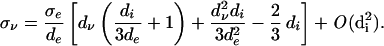
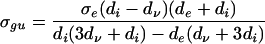
We can test the feasibility of the conductivity–diffusion cross-property relation predicted by Eq. 11 by comparing the relationship to the variational Hashin–Shtrikman (HS) bounds (25), which are the tightest bounds possible without taking into consideration any specific geometric properties of the tissue medium.‡‡ The HS bounds are specifically

13

Identifying λ with d and σ and eliminating φ_e we obtain the following greatest and least upper bounds on the conductivity eigenvalue, respectively, σ_gu and σ_lu, in terms of the diffusion eigenvalue

14

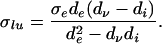15

Comparison of the above bounds with the predictions from the cross-property relation shows that the cross-property relation holds up even to intermediate values of intracellular diffusion (Fig. 1). To experimentally test the cross-property relation, particularly the prediction of strong linearity made by Eq. 12, diffusion tensor measurements were obtained and compared to reported invasive conductivity measurements in corresponding anatomical regions.

Figure 1.

Theoretical cross-property relationship between the conductivity and diffusion tensor eigenvalues normalized by the corresponding extracellular transport coefficient. The family of dotted curves gives the cross-property relationship for values of, from left to right, d_i/d_e = {0.1, 0.3, 0.5, 0.7}. The shaded regions indicate the greatest and least upper bounds predicted by the Hashin-Shtrikman (HS) bounds (25).

Methods

Axial, balanced echo (26) diffusion tensor measurements of four subjects were taken at 1.5 T (GE Signa) with TR/TE/τ = 3000/93/30 ms, b = 577.3 s/mm², 16 averages. Thirty-eight slices were obtained with a 40 × 20 cm² field-of-view (256 × 128) giving 1.56 × 1.56 × 3 mm³ voxels. The diffusion gradient (g = 14.14 mT/m) was applied in the directions of the six nonopposed edge-centers of a cube in k-space as described elsewhere (27).

The diffusion values were sampled in cortex, the parasagital sulcus, the anterior internal capsule, subcortical white matter, and the cerebellum. The locations were selected based on the locations of reported invasive conductivity measurements (28–32). The diffusion values were taken from either the frame or eigenframe depending on the anatomical direction in which the original invasive conductivity values were measured. If the full conductivity tensor was not specified, then the directions parallel and perpendicular to the fiber tract were taken to be, respectively, the directions of the major and minor eigenvectors. If the orientation of the conductivity measurement was not specified for a gray matter location, then the average eigenvalue of the diffusion tensor was used for comparison. The conductivity values were obtained from various species, but should still reflect the overall trend in the conductivity–diffusion relation.

Results

The full fractional linear relationship (Eq. 11) was fit to the conductivity and diffusion data, as was a linear relationship of the form σ_ν = k(d_ν − d_ɛ) for comparison. The former yielded σ_e = 1.52 ± 0.251 S/m, d_e = 2.04 ± 0.506 μm²/ms, and d_i = 0.117 ± 0.0972 μm²/ms. The uncertainty in the estimates for σ_e and d_e was principally due to the strong linear behavior in σ_e/d_e. The linear fit yielded k = 0.844 ± 0.0545 S⋅s/mm³ (P < 10⁻⁹) and d_ɛ = 0.124 ± 0.0540 μm²/ms (P < 0.05) with r² = 0.945. The linear relation provided a good approximation to the conductivity and diffusion data and could not be distinguished from the full fractional linear model based on the present data (Fig. 2). The linear relationship was used to generate the conductivity tensor image of the brain shown in Fig. 3.

Figure 2.

Experimental relationship between the conductivity and diffusion tensor eigenvalues (mean ± SEM). The conductivity values were obtained from reported invasive measurements and the diffusion values from diffusion tensor MRI in the corresponding anatomical regions. The solid line depicts the linear fit, and the dashed lines the upper and lower confidence intervals on the linear fit. The conductivity values were taken from the average over cortex (dark blue circle, ref. 28; red circle, ref. 31), the average subcortical white matter perpendicular to the tract (blue inverted triangle, ref. 28), somatosensory cortex in three perpendicular directions (yellow circle, ref. 30), the parasagital sulcus (light blue circle, ref. 29), the subcortical white matter beneath the parasagital sulcus measured perpendicular to the tract (light blue inverted triangle, ref. 29), the cerebellum parallel (green triangle) and perpendicular (green inverted triangle) to the dominant fiber orientation (32), and the anterior internal capsule parallel (purple triangle) and perpendicular (purple inverted triangle) to the tract (ref. 15).

Figure 3.

Axial electrical conductivity tensor map of the human brain derived from the linear cross-property relation. The region of interest is highlighted in the T2-weighted image shown at top left. The conductivity tensor within each voxel is represented by a three-dimensional ellipsoid. The axes of the ellipsoid are oriented in the direction of the conductivity tensor eigenvectors and are scaled by the corresponding eigenvalues. The length of the axis relative to the isotropic tensor (1 S/m; bottom right) gives the quantitative conductivity value. The color of the ellipsoid reflects the orientation of the principal eigenvector according to the red–green–blue sphere (top right) with red indicating mediolateral, green anteroposterior, and blue superoinferior. The brightness of the tensor is scaled by the degree of anisotropy. Note the strong anisotropy in the optical radiation (green), the tapetum (blue), and the U-fiber between the middle occipital and temporal gyri (red).

The conductivity data fell into three distinct clusters due to the sampling of the conductivity values in gray matter (i) and in white matter parallel (ii) and perpendicular (iii) to the fiber tract. To determine whether the linear relation could describe the behavior within these individual tissue classes, the linear model was also evaluated within the individual classes. The conductivity and diffusion values were not found to be significantly correlated (P > 0.05) within the tissue classes, indicating that the observed linearity followed primarily from the behavior across the tissue classes. It was not clear from the limited data available if the variability within the tissue classes was due to true disagreement with the model or experimental uncertainties such as anatomical heterogeneity, transspecies variability, and possible misspecification of the measurement orientation.

Discussion

We have derived a rigorous cross-property relation between the electrical conductivity and water self-diffusion tensors in brain tissue by relating the two transport processes through the statistical moments of the tissue microstructure. The cross-property relationship was found to respect theoretical bounds for a large range of intracellular diffusion values, and successfully captured the salient experimental observations: (i) a strong linear relation between the conductivity and diffusion eigenvalues, and (ii) a significant diffusion intercept at zero conductivity. The persistence of diffusion at zero conductivity can be understood by considering the following scenario. If the extracellular volume fraction is less than the percolation threshold (i.e., the extracellular space volume fraction at which the extracellular space is no longer topologically connected) the conductivity will vanish, but the diffusion will survive in the intracellular space and the disconnected extracellular pores. The surviving diffusivity at the percolation threshold will be on the order of the diffusion values d_i and d_ɛ derived here. Interestingly, these values are consistent with the “slow” diffusion component d_s = 0.168 μm²/ms observed at short diffusion times (33), which has been postulated to be the intracellular diffusion component. Furthermore, the value derived here for the extracellular conductivity is consistent with reported measurements for the conductivity of cerebrospinal fluid (σ = 1.79 S/m, ref. 34) and (σ = 1.54 S/m, refs. 35 and 36).

The quantitative conductivity tensor maps provided by the cross-property model promise to improve the accuracy of electromagnetic field modeling in tissue with application to a range of bioelectromagnetic technologies including electro/magnetoencephalography, electro/magnetocardiography, transcranial magnetic stimulation, and cardiac defibrillation. The cross-property framework will find particular application in the forward model for electromagnetic source imaging (ESI) where the empirical conductivity values will benefit both the accuracy and resolution of the source estimates. In particular, the inclusion of conductivity inhomoegeneities in the forward model will provide a basis for distinguishing sources inside or outside of the inhomogeneity.

The ability to quantify the currents based on the empirical conductivity measurements will furthermore allow for fusion of data from electric and magnetic imaging modalities. Because the electric and magnetic fields are sensitive to different source configurations and locations, the combination of modalities will help to further resolve the true underlying current distribution (11). Lastly, the cross-property framework is extendible to other transport and mechanical properties of tissue including thermal and acoustic conductivity, elastic stiffness, hydraulic permeability, and photon diffusion.

References

- 1.Plonsey R. Bioelectric Phenomena. New York: McGraw–Hill; 1969. [Google Scholar]
- 2.Haueisen J, Ramon C, Eiselt M, Brauer H, Nowak H. IEEE Trans Biomed Eng. 1997;44:727–735. doi: 10.1109/10.605429. [DOI] [PubMed] [Google Scholar]
- 3.Haueisen J, Bottner A, Nowak H, Brauer H, Weiller C. Biomed Tech (Berlin) 1999;44:150–157. doi: 10.1515/bmte.1999.44.6.150. [DOI] [PubMed] [Google Scholar]
- 4.Peters M J, De Munck J C. Acta Otolaryngol Suppl (Stockholm) 1991;491:61–68. doi: 10.3109/00016489109136782. [DOI] [PubMed] [Google Scholar]
- 5.Zhou H, van Oosterom A. IEEE Trans Biomed Eng. 1992;39:154–158. doi: 10.1109/10.121646. [DOI] [PubMed] [Google Scholar]
- 6.Klepfer R N, Johnson C R, Macleod R S. IEEE Trans Biomed Eng. 1997;44:706–719. doi: 10.1109/10.605427. [DOI] [PubMed] [Google Scholar]
- 7.Rudy Y, Plonsey R, Liebman J. Circ Res. 1979;44:104–111. doi: 10.1161/01.res.44.1.104. [DOI] [PubMed] [Google Scholar]
- 8.Metherall P, Barber D C, Smallwood R H, Brown B H. Nature (London) 1996;380:509–512. doi: 10.1038/380509a0. [DOI] [PubMed] [Google Scholar]
- 9.Wen H, Shah J, Balaban R S. IEEE Trans Biomed Eng. 1998;45:119–124. doi: 10.1109/10.650364. [DOI] [PMC free article] [PubMed] [Google Scholar]
- 10.Joy M, Scott G, Henkelman M. Magn Reson Imaging. 1989;7:89–94. doi: 10.1016/0730-725x(89)90328-7. [DOI] [PubMed] [Google Scholar]
- 11.Liu, A. K., Dale, A. M. & Belliveau, J. W. (2001) Hum. Brain Mapp., in press. [DOI] [PMC free article] [PubMed]
- 12.Tuch D S, Wedeen V J, Dale A M, George J S, Belliveau J W. Ann NY Acad Sci. 1999;888:314–316. doi: 10.1111/j.1749-6632.1999.tb07965.x. [DOI] [PubMed] [Google Scholar]
- 13.Basser P J, Mattiello J M, LeBihan D. Biophys J. 1994;66:259–267. doi: 10.1016/S0006-3495(94)80775-1. [DOI] [PMC free article] [PubMed] [Google Scholar]
- 14.Pierpaoli C, Basser P J. Magn Reson Med. 1996;36:893–906. doi: 10.1002/mrm.1910360612. [DOI] [PubMed] [Google Scholar]
- 15.Nicholson P W. Exp Neurol. 1965;13:386–401. doi: 10.1016/0014-4886(65)90126-3. [DOI] [PubMed] [Google Scholar]
- 16.Avellaneda M, Torquato S. Phys Fluids A. 1991;3:2529–2540. [Google Scholar]
- 17.Gibianksy L V, Torquato S. J Geophys Res (Solid Earth) 1998;103:23911–23923. [Google Scholar]
- 18.Gibianksy L V, Torquato S. Phys Rev Lett. 1993;71:2927–2930. doi: 10.1103/PhysRevLett.71.2927. [DOI] [PubMed] [Google Scholar]
- 19.Sen P N, Scala C, Cohen M H. Geophysics. 1981;46:781–795. [Google Scholar]
- 20.Brown W F. J Chem Phys. 1955;23:1514–1517. [Google Scholar]
- 21.Beran M J. Statistical Continuum Theories. New York: Wiley; 1968. [Google Scholar]
- 22.Sen A K, Torquato S. Phys Rev B. 1989;39:4504–4515. doi: 10.1103/physrevb.39.4504. [DOI] [PubMed] [Google Scholar]
- 23.Plonsey R, Heppner D B. Bull Math Biophys. 1967;29:657–664. doi: 10.1007/BF02476917. [DOI] [PubMed] [Google Scholar]
- 24.Milton G W. In: Physics and Chemistry of Porous Media. Johnson D L, Sen P N, editors. New York: Am. Inst. of Physics; 1984. [Google Scholar]
- 25.Hashin Z. J Mech Phys Solids. 1965;13:119–134. [Google Scholar]
- 26.Reese T G, Weisskoff R M, Wedeen V J. Proc Int Soc Magn Reson Med. 1998;6:663. [Google Scholar]
- 27.Reese T G, Weisskoff R M, Smith R N, Rosen B R, Dinsmore R E, Wedeen V J. Magn Reson Med. 1995;34:786–791. doi: 10.1002/mrm.1910340603. [DOI] [PubMed] [Google Scholar]
- 28.Freygang W H, Landau W M. J Cell Comp Physiol. 1955;45:377–391. doi: 10.1002/jcp.1030450305. [DOI] [PubMed] [Google Scholar]
- 29.van Harreveld A, Murphy T, Nobel K W. Am J Physiol. 1963;205:203–208. doi: 10.1152/ajplegacy.1963.205.1.203. [DOI] [PubMed] [Google Scholar]
- 30.Hoeltzell P B, Dykes R W. Brain Res. 1979;177:61–82. doi: 10.1016/0006-8993(79)90918-1. [DOI] [PubMed] [Google Scholar]
- 31.Ranck J B., Jr Exp Neurol. 1963;7:144–152. doi: 10.1016/s0014-4886(63)80005-9. [DOI] [PubMed] [Google Scholar]
- 32.Nicholson C, Freeman J A. J Neurophysiol. 1975;38:356–368. doi: 10.1152/jn.1975.38.2.356. [DOI] [PubMed] [Google Scholar]
- 33.Niendorf T, Dijkhuizen R M, Norris D G, van Lookeren Campagne M, Nicolay K. Magn Reson Med. 1996;36:847–857. doi: 10.1002/mrm.1910360607. [DOI] [PubMed] [Google Scholar]
- 34.Baumann S B, Wozny D R, Kelly S K, Meno F M. IEEE Trans Biomed Eng. 1997;44:220–223. doi: 10.1109/10.554770. [DOI] [PubMed] [Google Scholar]
- 35.Geddes L A, Baker L E. Med Biol Eng. 1967;5:271–293. doi: 10.1007/BF02474537. [DOI] [PubMed] [Google Scholar]
- 36.Roth B J, Altman K W. Med Biol Eng Comput. 1992;30:103–108. doi: 10.1007/BF02446201. [DOI] [PubMed] [Google Scholar]