Abstract
Detailed knowledge of vegetation structure is required for accurate modelling of terrestrial ecosystems, but direct measurements of the three dimensional distribution of canopy elements, for instance from LiDAR, are not widely available. We investigate the potential for modelling vegetation roughness, a key parameter for climatological models, from directional scattering of visible and near-infrared (NIR) reflectance acquired from NASA’s Moderate Resolution Imaging Spectroradiometer (MODIS). We compare our estimates across different tropical forest types to independent measures obtained from: (1) airborne laser scanning (ALS), (2) spaceborne Geoscience Laser Altimeter System (GLAS)/ICESat, and (3) the spaceborne SeaWinds/QSCAT. Our results showed linear correlation between MODIS-derived anisotropy to ALS-derived entropy (r2= 0.54, RMSE=0.11), even in high biomass regions. Significant relationships were also obtained between MODIS-derived anisotropy and GLAS-derived entropy (0.52≤ r2≤ 0.61; p<0.05), with similar slopes and offsets found throughout the season, and RMSE between 0.26 and 0.30 (units of entropy). The relationships between the MODIS-derived anisotropy and backscattering measurements (σ0) from SeaWinds/QuikSCAT presented an r2 of 0.59 and a RMSE of 0.11. We conclude that multi-angular MODIS observations are suitable to extrapolate measures of canopy entropy across different forest types, providing additional estimates of vegetation structure in the Amazon.
Keywords: canopy roughness, multi-angle, MODIS, MAIAC, LiDAR, anisotropy
1. Introduction
Terrestrial vegetation plays a significant role in the re-distribution of moisture and heat in the surface boundary layer, as well as in the energy balance of the planet (Bastiaanssen et al., 1998a). Land-atmosphere interactions are driven by the three-dimensional structure of vegetated land cover, including surface roughness, leaf area and canopy volume (Vourlitis et al., 2015; Domingues et al., 2005). Canopy roughness, defined as vertical irregularities in the height of the canopy (Chapin et al., 2011), plays a key role in earth system modelling. For instance, evapotranspiration is controlled much more by canopy roughness (and therefore aerodynamic conductance) than by canopy leaf area or maximum stomatal conductance (Chapin et al., 2011).
At stand level scales, significant advances have been made measuring canopy vegetation structure from Light Detection and Ranging (LiDAR). LiDAR allows direct measurements of the three-dimensional distribution of vertical vegetation elements from ground-based (Strahler et al., 2008), airborne (Wulder et al., 2012) and orbital platforms (Sun et al., 2008). To date, most vegetation related LiDAR applications rely on airborne platforms for data acquisition, with measurements acquired at altitudes between 500 and 3000 m (Hilker et al., 2010). Due to cost and practical considerations, the availability of airborne LiDAR is currently limited to specific research sites and data are not available across the landscape.
The Geoscience Laser Altimeter System (GLAS), onboard the Ice, Cloud, and land Elevation Satellite (ICESat), has provided certain capability to map vegetation characteristics across broader areas from space (Zwally et al., 2002). GLAS is a large-footprint, waveform-recording LiDAR that measures the timing and power of the 1064 nm laser energy returned from illuminated surfaces (Schutz et al., 2005). While not configured for vegetation characterization, the GLAS instrument allows quantification of the vertical distribution of plant components relative to the ground over vegetated terrain (Harding, 2005; Yu et al., 2015, Morton et al., 2014). GLAS data has been successfully used to discriminate forest structure across various biome types (Boudreau et al., 2008; Gonçalves, 2014; Lefsky et al., 2005; Pang et al., 2008) and to estimate canopy light environments and forest productivity (Stark et al., 2014; Rap et al., 2015; Morton et al., 2016). While GLAS provides larger spatial coverage, its footprint is still spatially discrete and importantly a lack of repeated measurements prevents its use for estimation of climate related responses of vegetation.
Perhaps complimentary to structural observations, optical remote sensing available from satellite data, provide global coverage at frequent time steps but can generally not deliver accurate information on the vertical organization of plant canopies. For instance, vegetation indices provide general information on canopy “greenness” but their ability to detect changes in high-biomass areas is limited due to a well-documented saturation effect (Carlson and Ripley, 1997). Although VIs have been employed as proxies for vegetation structure, including roughness lengths for turbulent transfer, field estimates of vegetation structure attributes are often only moderately correlated with VIs and their derivatives (Glenn et al., 2008).
As an alternative to conventional, mono-angle observations, the combination of multiple view angles may provide new opportunities for modelling the structure of vegetated land surfaces (Breunig et al., 2015; Shaw & Pereira, 1982) from optical remote sensing. Changes in canopy structure including changes in tree crown size, shape, density and spatial distribution of leaves, affect the directional scattering of light (Chen et al., 2005). Multi-angle observations of this scattering may therefore allow us to describe the three-dimensional structure of vegetation (Chen and Leblanc, 1997; Strahler & Jupp, 1990). Multi-angular scattering of surface reflectance (anisotropy) has been linked to optical properties and geometric structure of the target (Widlowski et al., 2004; Widlowski et al., 2005), including canopy roughness (Strahler, 2009), leaf angle distribution (Roujean, 2002), leaf area index (LAI) (Walthall, 1997) and foliage clumping (Chen et al., 2005; Chopping et al., 2011). Such estimates may even be made in dense canopies (Moura et al., 2015), as observations acquired from multiple view angles decrease the dispersion and saturation effect in geometrically complex vegetation (Zhang et al., 2002).
With the advent of multi-angular sensors such as the Multi-angle Imaging SpectroRadiometer (MISR) (Breunig et al., 2015) and POLDER (Roujean, 2002), the dependence of reflectance on observation angles has been documented (Barnsley et al., 2004) and modelled (Roujean et al., 1992; Wanner et al., 1995). Recent progress using the Multi-Angle Implementation of Atmospheric Correction Algorithm (MAIAC) has allowed the acquisition of multi-angle reflectance across large areas and at high observation frequencies by combining satellite imagery obtained from NASA’s Moderate Resolution Imaging Spectroradiometer (MODIS) Terra and Aqua platforms during a few overpasses (Lyapustin et al., 2012a; Moura et al., 2015). Such observations could potentially allow periodic and spatially contiguous estimates of vegetation structure and its response to changes in climate variables. When correlated with more direct measurements of canopy structure by other instruments, such as LiDAR, this may then allow us to extrapolate canopy roughness and other structural estimates in space and time, thereby filling key data gaps for improving our understanding of ecosystem structure and functioning. Further validation may be provided by scatterometer observations over dense forests. For instance, the SeaWinds microwave radar, onboard NASA’s QuikSCAT satellite, was primarily designed to measure near-surface wind speed and direction over the oceans. However, due to its high sensitivity to water content that drives canopy dielectric properties, it has been also used to study canopy structure (Frolking et al., 2011; Saatchi et al., 2013).
In this study, we used estimates of canopy roughness obtained from 1) airborne laser scanning (ALS), 2) spaceborne LiDAR GLAS, and 3) the spaceborne SeaWinds scatterometer, to evaluate the potential of multi-angular MODIS observations for modelling vegetation roughness from directional scattering of visible and near-infrared (NIR) reflectance. We implemented a spatial scaling approach, from airborne to orbital levels of data acquisition, to model continuous coverage of roughness across tropical forests of the Xingu basin area in the Brazilian Amazon. Our objective was to test whether multi-angle MODIS reflectance can be used as a proxy for canopy roughness over Amazonian tropical forests, including different forest types such as Dense and Open ombrophilous Forests, and Semi-Deciduous Forest.
2. Methods
2.1. Study area
The study area is located in the southeast part of the Amazon, including the Xingu basin and adjacent areas (Figure 1). Figure 1 also shows the GLAS transects for the study area (Schutz et al., 2005) as well as the ALS and the field data plots. The study area presents a south-north gradient with respect to climate. Following the Kӧppen classification, the southern portion of the study area is dominated by tropical wet and dry climate (Aw), while the north portion is characterized by tropical monsoon climate (Am). Length and duration of the dry season, defined as months with rainfall less than 100 mm or less than one third of precipitation range (Asner & Alencar, 2010; Myneni et al., 2007), also varies across the study area. In the southern parts, the dry season lasts about five months, from May to September (Moura et al., 2012). In the northern parts, a drier climate prevails between July and November (Vieira et al., 2004). The area is characterized by three predominant forest types: Dense Ombrophilous Forest (Dse), Open Ombrophilous Forest (Asc) and Semi-Deciduous Forest (Fse) (IBGE, 2004).
Figure 1.
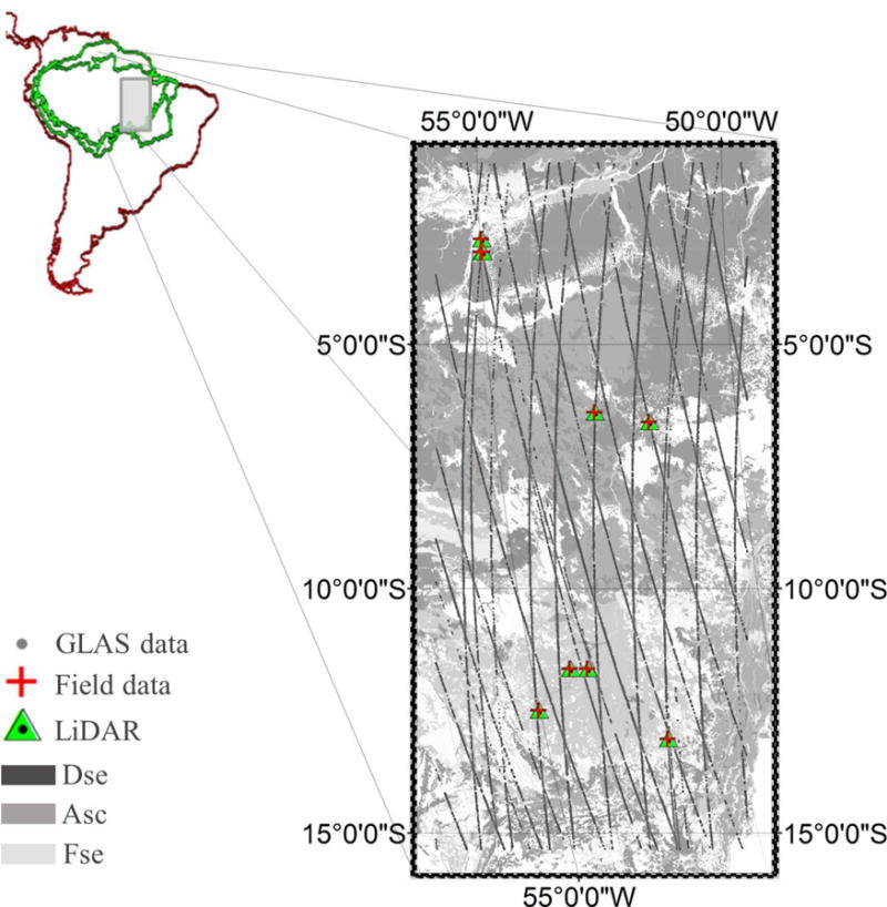
Location of the study within the Amazon basin. The inset shows the Geoscience Laser Altimeter System (GLAS) coverage (strings), airborne laser scanning (ALS) data acquisition and the available field inventory plots across the Xingu basin.
2.2. Field inventory data
Estimates of vegetation structure were derived for each of the three different forest types using available inventory plots across the region. For two vegetation types, Open Ombrophilous Forest (Asc) and Semi-decidiuous Forest (Fse), surveys were provided by the Sustainable Landscapes Brazil project in collaboration with the Brazilian Agricultural Research Corporation (EMBRAPA), the US Forest Service, the USAID, and the US Department of State (http://mapas.cnpm.embrapa.br/paisagenssustentaveis/). The Asc forest type was represented by 22 plots of 40 m × 40 m each. All the trees with a diameter at breast height (DBH) equal to or greater than 10 cm were measured within each plot. For Fse, 10 sample plots (20 m × 500 m) were used. The field data for the Dense Ombrophilous Forest (Dse) were obtained in 2012 and are described in Silva et al. (2015). The floristic and structural surveys included seven sample plots of 25 m × 100 m over mature forests. Trees with DBH equal to or greater than 10 cm were measured within each plot.
2.3. Airborne Laser Scanning (ALS) data
ALS data were acquired by GEOID Ltd. using an Altm 3100/Optech instrument and provided by the Sustainable Landscapes Brazil project. The positional accuracy (1σ) of the LiDAR measurements was approximately 0.10 m horizontally and 0.12 m vertically (http://mapas.cnpm.embrapa.br/paisagenssustentaveis/). We focussed our analysis on undisturbed, non-degraded research plots. Structural information was obtained in the Tapajós National Forest, Pará State (September to November 2012), in São Félix do Xingu municipality, Pará state (August 2012) and in Canarana/Querência municipality, Mato Grosso State (August 2012), to represent Dse, Asc and Fse, respectively. Table 1 shows the specifications of LiDAR data for each site.
Table 1.
Characteristics of the airborne laser scanning (ALS) data acquired over Dense Ombrophilous (Dse), Open Ombrophilous (Asc) and Semi-Deciduous (Fse) Forests in the Brazilian Amazon.
| Forest Type | Total area (ha) | Max flight altitude (m) | Flightline overlap (%) | Average return density (ppm2) | Average first return density (ppm2) | Field of view (°) |
|---|---|---|---|---|---|---|
| Dse | 1049 | 850 | 65 | 25.1 | 15.28 | 11.1 |
| Asc | 1004 | 850 | 65 | 24.1 | 15.20 | 11.0 |
| Fse | 1005 | 850 | 65 | 13.7 | 7.05 | 11.0 |
ALS data were delivered as classified LAS-formatted point clouds, along with 1-m resolution bare earth digital terrain models (DTM). For comparison with GLAS, discrete-return data were aggregated produce pseudo-waveforms. Coops et al. (2007) demonstrated that canopy profiles, analogue to those derived from full waveform systems, can be derived from discrete return LiDAR when aggregating returns into three dimensional voxel spaces and comparing the amount of discrete returns contained in each voxel layer to the voxel layers below and above. In this study, waveforms were synthesized by sub-setting the LiDAR point cloud co-located with each field plot and counting the number of points observed in vertical bins of 50 cm and at a horizontal resolution of 100 ×100m. 10 by 10 pixels of LiDAR metrics were then averaged to match the 1×1km MODIS pixel size. ALS based entropy was then computed to determine canopy structural diversity and approximate canopy roughness (Palace et al., 2015; Stark et al., 2012). The method is described in detail in the next section (2.4) and is analogue to that applied from GLAS observations. In addition to ALS entropy, we also calculated canopy volume models (CVMs) to quantify the three-dimensional structure of the forest canopies based on the incident radiation levels and photosynthetic potential (Coops et al., 2007; Hilker et al., 2010). The method is described in detail in (Lefsky et al., 2005). CVMs divide the canopy space into sunlit and shaded vegetation elements as well as gap spaces enclosed within.
2.4. GLAS/ICESat data and structural metrics from vertical profiles
GLAS profiles were obtained across the Xingu basin (Figure 1) between 2006 and 2008 (laser operating periods 3E through 2D) (Gonçalves, 2014). Each GLAS footprint is elliptical in shape, spaced at approximately 170-m intervals along-track. GLAS LiDAR profiles characteristics varied between the campaigns across the study area. The near-infrared elliptical footprint and eccentricity varied between 51.2 (±1.7) to 58.7 (±0.6), and 0.48 (±0.02) to 0.59 (±0.01), respectively. The horizontal and vertical geolocation accuracy varied between 0.00 (±3.41) to 1.72 (±7.36), and 0.00 (±2.38) to 1.2 (±5.14), depending on the campaign and respective data product.
Because GLAS observations are able to penetrate optically thin clouds (Schulz et al., 2005), processing of the GLAS profiles included additional cloud screening to improve the data quality. The technique is described in detail in Smith et al. (2005). Briefly, the approach takes advantage of the fact that returns unaffected by saturation or forward scattering resemble narrow Gaussian pulses that are similar to the transmitted pulse (Smith et al., 2005). To process GLAS waveforms, we used parameters reported in the GLA01, GLA05, and GLA14 data products following methods described by (Gonçalves, 2014). First, the waveforms were filtered by convolution with a discrete Gaussian kernel with the same standard deviation as the transmitted laser pulse. This procedure reduced the background noise, while preserving an adequate level of detail for characterization of the canopy (Sun et al., 2008). Second, GLAS waveforms used in this study were calibrated and digitized into 1000 discrete bins at a time resolution of 1 ns (~15 cm). The locations of the highest (signal start) and lowest (signal end) detected surfaces within the 150-m waveform were determined, respectively, as the first and last elevations at which the amplitude exceeded a threshold level, for a minimum of n consecutive bins. The peak of the ground return was determined as the lowest peaks in the smoothed waveforms with at least the same width as the transmitted laser pulse, after taking into account the mean noise level. In order to minimize the effect of different output energy levels of the 2E and 3E Laser flight campaigns, all profiles were then normalized to unity by dividing by the maximum amplitude. This correction approach assumes that differences in measurement campaigns affect the overall amount of energy but do not significantly change the waveforms (i.e. the vertical scale of energy output) of our entropy calculation (Gonçalves, 2014).
We utilized GLAS estimates of entropy (Sz), a measure of canopy structural diversity sensitive to crown depth and leaf area (Palace et al., 2015; Stark et al., 2012), as a proxy of canopy roughness. Sz was calculated using Equations 1 and 2 (Harding & Carabajal, 2005, Nelson et al., 2009, Treuhaft et al., 2009, Gonçalves, 2014):
| (1) |
| (2) |
where nb is the number of vertical bins from the ground peak to the signal start defined as the vertical distance between the ground peak and the signal start; w(z) is the laser power received from the 1m bin centered at height z; H100 is the maximum canopy height, defined as the vertical distance between the ground peak and the signal start (Gonçalves, 2014).
2.5. SeaWinds/QuikSCAT data
Estimates of canopy structure were independently also obtained from SeaWinds Scatterometer data, provided by NASA’s Scatterometer Climate Record Pathfinder project. The SeaWinds Scatterometer operates at microwave frequency of 13.4 GHz (Ku-band) with mean incidence angle of 54° for V-polarization and 46° for H-polarization. The sensitivity of radar data to variations in vegetation canopy structure can be explained by the dependence of radar backscatter to surface dielectric properties, which are strongly dependent on the liquid water content of the canopy constituents (Frolking et al., 2006). Given that the SeaWinds instrument operates at a higher frequency and higher incidence angle than other similar sensors, it has lower penetration into forest canopy, and therefore almost no interference from soil moisture variations in densely vegetated forested areas (Saatchi et al., 2013).
The backscatter product (σ0) used in this study combines ascending (morning) and descending (evening) orbital passes, and is based on SeaWinds “egg” images (Frolking et al., 2006). The nominal image pixel resolution for egg images is 4.45 km/pixel. Only backscatter data for horizontal (H) polarization were used, as previous assessments had indicated that results using vertical (V) polarization show no significant differences (Saatchi et al., 2013). We used data obtained from January 2001 to November 2009, when the sensor stopped collecting data due to failure in the scanning capability. To match the spatial resolution of the SeaWinds instrument, we averaged the corresponding anisotropy observations from the MODIS instrument to match the SeaWinds/QuikSCAT pixels.
2.6. Determination of surface anisotropy from multi-angle MODIS data
MODIS observations are acquired at different solar and view zenith angles, depending on the orbital overpass and time of the year. Pixel-based algorithms often assume a Lambertian reflectance model, which reduces the anisotropy of the derived surface reflectance (Lyapustin, 1999; Wang et al., 2010), thus decreasing the ability to detect directional scattering (Hilker et al., 2009). In this study, we use the MAIAC algorithm because it preserves the multi-angle character of MODIS observations, providing a means to estimate the anisotropy of surface reflectance (Chen et al., 2005), a surrogate for structure of vegetation and shaded parts of the canopy (Myneni et al., 2002; Chen et al., 2003; Gao et al., 2003). MAIAC is a cloud screening and atmospheric correction algorithm that uses an adaptive time series analysis and processing of groups of pixels to derive atmospheric aerosol concentration and surface reflectance. A detailed description of the technique can be found in Lyapustin et al. (2011) and Lyapustin et al. (2012). Previous results (Hilker et al., 2012, 2015) have shown that while the MAIAC cloud mask is less conservative, it is also more accurate, improving the number of observations and data quality in tropical environments.
For retrieval of the surface bi-directional reflectance distribution function (BRDF), MAIAC accumulates data over 4-16 days (Lyapustin et al., 2011 Lyapustin et al., 2012). Assuming that vegetation is relatively stable during this period, the surface directional scattering can be characterized using the Ross-Thick Li-Sparse (RTLS) bidirectional reflectance distribution function (BRDF) model (Roujean, et al., 1992).
Using the RTLS model (Wanner et al., 1995), we characterized the BRDF of each 1 km × 1 km grid cell of MODIS data. Based on the RTLS BRDF model, we derived MODIS backscatter (Solar Zenith Angle (SZA) = 45°, View Zenith Angle (VZA) = 35°, Relative Azimuth Angle (RAA) = 180°) and forward scatter (SZA = 45°, VZA = 35°, RAA = 0°) observations (4-16 days of observations) for a fixed view and sun angle. The advantage of using the RTLS model rather than reflectance directly is to keep constant sun-observer geometry and extrapolate measurements to the principal plane. In addition, the modelled reflectance can be based on all multi-angle MODIS data, which should yield a more representative characterization of the reflectance properties. We selected a VZA of 35° rather than the hotspot location at VZA = 45° in order to keep the modelled reflectance closer to the actual range of angles observed by MODIS, thereby minimizing potential errors resulting from extrapolation of the BRDF.
We used estimates of anisotropy (defined as the difference between BRDF modelled backscattering (SZA = 45°, VZA = 35°, RAA = 180°) and BRDF modelled forward scattering (SZA = 45°, VZA = 35°, RAA = 0°) based on the Enhanced Vegetation Index (EVI) to describe roughness of the surface for different vegetation types across the study area (Moura et al., 2015). The objective of using EVI rather than surface reflectance of a given band was to minimize the effect of non-photosynthetically active elements (i.e. soil fraction component) while optimizing the sensitivity to green canopy structure (Moura et al., 2015).
MODIS-derived anisotropy values were then regressed against ALS-derived entropy, GLAS-derived entropy and SeaWinds/QuikSCAT backscatter (σ0, Frolking et al., 2006), which were estimated on a per-pixel-basis to generate time series profiles of entropy for each forest type in the study area.
3. Results
The Xingu basin contains a number of different forest types. However, vegetation is dominated by Asc and Dse forest types in the north, and by Fse vegetation in the south, as illustrated in Figure 2. The GLAS tracks are also shown in this figure to highlight the sampling density of the spaceborne LiDAR over each forest type. An illustration of the mean canopy height (MCH) derived from ALS for three sample areas of 1 ha each is provided in Figure 2. Airborne ALS measurements showed, on average, the largest tree heights in the Dse class with values up to 40 meters tall (red color in the inset of Figure 2). Asc and Fse vegetation types reached up to 30 m and 25 meters in height, respectively. Field measurements showed that mean canopy heights from forest inventories were 19.8 m, 17.4 m and 17.0 m for Dse, Asc and Fse, respectively (Table 2). When compared to Asc and Fse, Dse presented larger metrics of diversity (i.e. species richness (S) and Shannon index (H’)) and structure (mean height (HT), mean diameter at breast height (DBH), basal area (BA), aboveground biomass (AGB) and leaf area index (LAI)) (Table 2).
Figure 2.
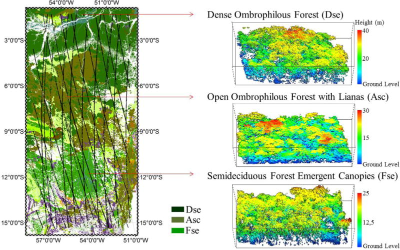
Vegetation cover map adapted from IBGE (2004) in the left, and diagrams of height estimates from ALS LiDAR data in the right, to illustrate structural variation between the three predominant forest types in the study area (Dse, Asc and Fse). Each Airborne Laser Scanning (ALS) plot represents an area of 100 m ×100 m to describe the heights in the three different forests.
Table 2.
Floristic and structural metrics calculated from field inventory data for Dense Ombrophilous Forest (Dse), Open Ombrophilous Forest (Asc) and Semi-Deciduous Forest (Fse). The mean leaf area index (LAI), determined from Airborne Laser Scanning (ALS), is indicated in the last column of the table.
| Forest Type | Plots | S | H′ | Ht(m) |
|
LAI(ALS) | |
|---|---|---|---|---|---|---|---|
| Dse | 7 | 181 | 4.61 | 18.1 | 30.63 | 6.05 | |
| Asc | 22 | 1595 | 3.67 | 17.4 | 11.36 | 4.32 | |
| Fse | 10 | 802 | 2.20 | 17.0 | 12.83 | 5.33 |
Differences in canopy structure were also evident from the analysis of canopy volume models (CVMs) (Figure 3). While gap spaces were relatively small in all three vegetation types, Asc showed a notably higher proportion of sunlit vegetation that reached down deep into the canopy, suggesting a higher spatial variability of tree heights compared to the other two vegetation types. Similarly, gaps in the upper canopy were mostly present in Asc, as expected for open forest types. Fse showed gaps predominantly in lower height levels, and a higher overall proportion of shaded crown. Full canopy closure (100% of the canopy space filled by either sunlit or shaded canopy elements or fully enclosed gap space) was reached at about 15 m height for both Asc and Dse, and at about 20 m height for Fse.
Figure 3.
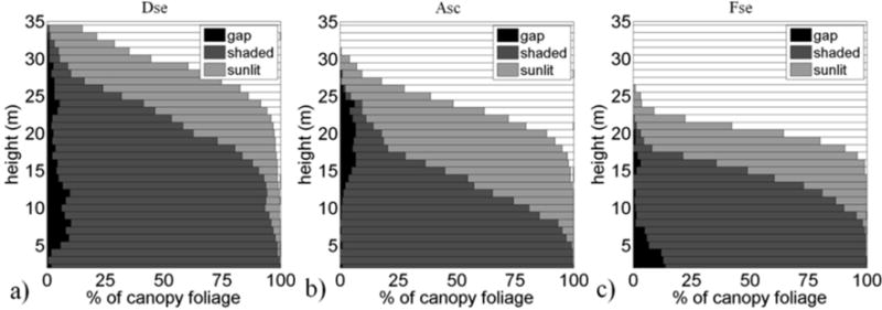
Canopy volume models (CVMs) based on the Airborne Laser Scanning (ALS) for (a) Dense ombrophilous forest (Dse); (b) Open ombrophilous Forest (Asc); and (c) Semi-deciduous forest (Fse).
Differences in vegetation structure derived from ALS data were confirmed also with spaceborne GLAS observations. GLAS-derived seasonal profiles of entropy for 2006 showed spatial averages that differed over time between the three vegetation types (Figure 4). Even though there were differences in the years of data acquisition (2006 for GLAS and 2012 for ALS), the shaded area in Figure 4 was plotted to provide a seasonal reference between the airborne and spaceborne data. GLAS derived seasonal profiles varied between different forest types. The lowest values of entropy were consistently found for Fse. In contrast, Asc for Dse showed GLAS entropy higher throughout the measurement period. All forest types showed strong seasonality with increasing entropy from February to September, and decreasing values thereafter with predominance of higher entropy during the dry season.
Figure 4.
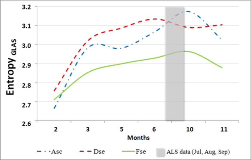
Seasonal profiles of GLAS-derived entropy for the three different forest types of the study area. GLAS data were obtained only for the months indicated in the x-axis. Just for reference, the shaded area represents the quarter when the Airborne Laser Scanning (ALS) data were collected in 2012.
Examples of MODIS anisotropy during March, June and October of 2006 illustrated seasonal and spatial changes in multi-angle reflectance across the Xingu basin (Figure 5). The MODIS derived anisotropy was consistently higher in the northern part of the study area, and its spatial distribution coincided well with the forest types indicated in Figure 2. A clear limit between forested (high MODIS anisotropy) and non-forested (low anisotropy) areas was evident in the southern part of the map. Furthermore, higher values of anisotropy were found for the Asc and Dse vegetation compared to Fse. While MAIAC observations allowed a notable number of measurements of anisotropy between June (Figure 5b) and October (Figure 5c), some data gaps were observed in March (Figure 5a) due to cloud cover in the rainy season.
Figure 5.
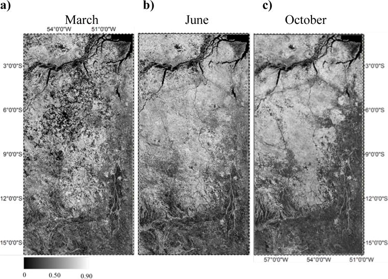
MODIS-derived anisotropy images during (a) March, (b) June and (c) October of 2006 to illustrate seasonal and spatial changes in multi-angle reflectance across the Xingu basin.
MODIS-derived anisotropy was linearly correlated to ALS-derived entropy (Figure 6). The coefficient of determination (r2) of the relationship between all 828 MODIS pixels that coincided with existing ALS observations was 0.54 with an RMSE of 0.11 units of entropy. Much of the scattering presented in Figure 3 was limited to lower values of entropy, while residuals were notably smaller for the higher entropy range.
Figure 6.
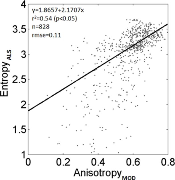
Relationship between MODIS-derived anisotropy and ALS-derived entropy (or canopy roughness).
Significant relationships were also found between MODIS anisotropy and GLAS measured entropy using all observations that contained five or more GLAS shots within the 1 km × 1 km MODIS pixels (Figure 7). In order to examine seasonal variability in the relationship, we performed the regressions separately for March (Figure 7a), June (Figure 7b) and October (Figure 7c) of 2006. The r2 varied between 0.52 for March and 0.61 for June (p<0.05) with similar slopes and offsets found throughout the observation period. RMSE varied between 0.26 and 0.30 units of entropy. The highest noise levels were observed in March, which is corresponding also to the larger amount of data gaps during the rainy season (Figure 5). The availability of GLAS data was somewhat limited during June, but the relationships were still highly significant and consistent with those observed during other months of the year. A comparison between conventional VI estimates using directionally normalized EVI from MAIAC and LiDAR derived Entropy is shown in the appendix (Figure A1).
Figure 7.
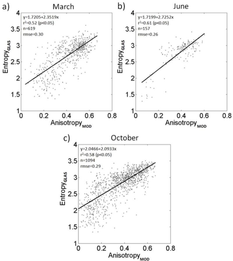
Relationship between MODIS-derived anisotropy and GLAS-derived entropy using observations for (a) March, (b) June and (c) October of 2006.
A strong relationship between the MODIS-derived anisotropy and the backscattering measurements (σ0) from SeaWinds/QuikSCAT was also observed (Figure 8). The relationship was obtained for 10.000 randomly sampled MODIS pixels and corresponding SeaWinds/QuikSCAT (σ0) observations across the Xingu basin for all available QuikSCAT data between 2001 and 2009. Note, however, that when using radar observations, the relationship to MODIS-derived anisotropy was non-linear (r2=0.59, RMSE=0.11).
Figure 8.
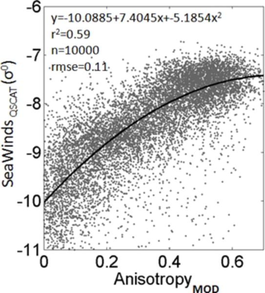
Relationship between MODIS-derived anisotropy and backscattering (σ0) measurements from SeaWinds/QSCAT over Amazonian tropical forests considering the period 2001 to 2009.
Time series profiles of MODIS-derived entropy estimated from the regression model of Figure 7c and of MODIS-derived QuikSCAT-σ0 estimated from model of Figure 8 were plotted as spatial averages for Dse, Asc and Fse (Figure 9). All three forest types displayed notable seasonal cycles. The Ombrophilous Forests (Dse and Asc) consistently showed high values of entropy with less seasonal variation. In contrast, the seasonal cycles were much more pronouced in the Fse, as expected for semi-decidous vegetation. Both models (GLAS-derived entropy and QScat-derived σ0) yielded very similar seasonal patterns, in terms of temporal variation as well as in terms of differences between vegetation types. The results presented in Figure 9 were consistent also with those shown in Figure 5. A small negative trend in both entropy and σ0 was observed from 2000 until 2009 and a positive trend in all three vegetation types was found from 2010 onwards. This trend was especially pronounced for the canopy entropy based on GLAS observations.
Figure 9.
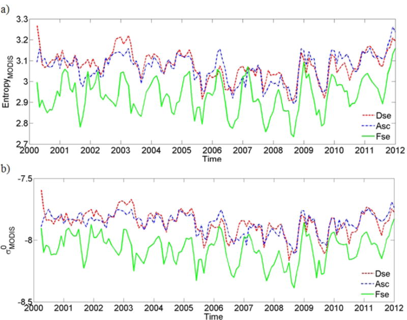
Time series profiles of MODIS-derived (a) GLAS entropy estimated using the regression model of Figure 7c, and (b) MODIS-derived SeaWinds/QuikSCAT backscattering (σ0) from the model of Figure 8. Results are shown as spatial average for Dense (Dse) and Open (Asc) Ombrophilous Forests and the Semi-Deciduous Forest (Fse) between 2000 and 2012 for the Xingu basin.
4. Discussion
This study investigated the potential of multi-angle reflectance obtained from MODIS to derive estimates of vegetated surface roughness as an important structural parameter of land atmosphere interactions. Aside from field observations, airborne laser scanning is arguably the most comprehensive tool to describe the three-dimensional vegetation structure at the stand level to date (Coops et al., 2007; Lim et al., 2003; Wulder et al., 2012). Recent initiatives such as the “Sustainable Landscapes Brazil“ project (http://mapas.cnpm.embrapa.br/paisagenssustentaveis/) seek to improve upon existing deficiencies of data availability and provide new opportunities to generate structural metrics across discrete locations within the Amazon basin.
LiDAR based characterization of vegetation structure (Figures 2, 3, and Table 1) exposed a large heterogeneity across the Xingu basin, both spatially and seasonally. ALS-observed structural differences between vegetation types were detectable also from space using photon counting LiDAR (GLAS/IceSat) and microwave backscattering (SeaWinds/QuikSCAT) (Figures 4 and 9b). This is an important finding, as it opens an opportunity for scaling spatially discrete observations of canopy structure across larger areas from space (Popescu et al., 2011).
Spatial and temporal heterogeneity in Amazonian vegetation (Silva et al., 2013; Townsend et al., 2008) is not easily obtained from conventional vegetation indices (Hilker et al., 2015), as VIs cannot adequately capture differences in canopy structure among different vegetation types (Glenn et al., 2008; Lagouarde et al., 2002). Findings presented in this study (Figures 6 to 9) suggest that such canopy structural variation may be better determined from multi-angular reflectance. Our estimates of anisotropy showed considerable improvements over estimates using mono-observation vegetation indices (Figure A1). The ability of multi-angle observation to derive vegetation structural attributes is well supported by previous results (Chen & Leblanc, 1997; Chen, 2003; Gao, 2003; Strahler & Jupp, 1990; Yu et al., 2015; Zhang et al., 2002). While these authors have focused on smaller study areas using specialized sensors, our findings confirm such multi-angle potential to be acquired from the MODIS instrument and across the Amazon basin (Moura et al., 2015). Our previous work also confirmed the consistency of monthly anisotropy measurements and its statistical significance for estimating seasonal changes in vegetation structure across the Amazon (Moura et al., 2015). This is an important advancement, as it allows structural estimates over large areas and at high temporal frequencies from space, complementing the data analysis of orbital LiDAR data.
Anisotropy derived from multiple overpasses of MODIS imagery may therefore provide new insights into structural variability of Amazon forests as it increases the sensitivity to changes in vegetation structure across dense vegetation types. As demonstrated in previous work (Moura et al., 2015), seasonal changes in observed anisotropy cannot be explained by bi-directional effects, as all observations have been normalized to a fixed forward and backscatter geometry (Lyapustin et al., 2012b). In addition, Moura et al. (2015) demonstrated that standard deviations between observed and modelled MAIAC reflectance were about 10% of the observed variation in anisotropy, thus confirming the ability of our approach to detect seasonal and inter-annual changes. Differences between forward and backscatter observations as utilized in this paper are largely driven by the different directional scattering behaviour of red and NIR reflectance (Moura et al., 2015, Hilker et al., 2015). The modelled near hotspot and near darkspot locations were designed to maximize the range of resulting anisotropy, thereby seeking to increase the sensitivity with respect to changes in vegetation structure.
While the range of view angles acquired by MODIS is relatively small, as the instrument was not specifically designed for multi-angle acquisitions, MODIS-derived anisotropy still provided an effective means to characterize vegetation structure across large areas from space. Within the Amazon basin (or tropics in general), this is partially facilitated by the fact that MODIS view geometry comes very close to the principal plane twice a year. As a result, our BRDF model is representative of the angles used in this study. Consequently, modelled anisotropy is close to its maximum range of possible values. The contrary occurs in mid-latitudes where observations are further from the principal plane. In these cases, other geometric configurations might be preferable.
Modelling MODIS anisotropy using the RTLS BRDF model further allowed us to derive anisotropy independent of the sun-observer geometry (Roujean et al., 1992). As a limitation to this approach, changes in sun-sensor configuration over the year do not always allow modelling of forward and backscattering observations within the sampling range of the MODIS instruments. Therefore, higher uncertainties may be observed during some times of the year than during others.
The strong, positive correlation found between GLAS-measured entropy and MODIS anisotropy (Figure 6) may be explained by geometric scattering of individual tree crowns (Chopping et al., 2011; Li, X., Strahler, 1986). For instance, a large variability in canopy heights (high canopy roughness) will increase the geometric scattering component, especially of NIR reflectance. Other structural changes may, however, also influence seasonal patterns of anisotropy. In addition to canopy roughness, anisotropy is also affected by leaf angle distribution (Roujean, 2002) and foliage clumping (Chen et al., 2005) among other variables related to the floristic variability, which tends to be high in tropical forests. The interaction between these variables and multi-angle scattering is not straightforward, requiring further investigation, especially in the components of scattering determined in the RTLS model. For example, increases in leaf area may increase the volumetric scattering component (Ross, 1981; Roujean, et al., 1992) of multi-angle reflectance, but at the same time decrease the surface roughness, at least within a certain range of values. Therefore, the results presented in here should be understood as a first demonstration of the technique.
Due to the complexities described as well as other limitations in terms of footprint size, and range of angular sampling, MODIS-derived estimates of canopy structure should not be understood as a replacement for direct 3D measures of vegetation, but rather as a complimentary approach for scaling such observations in space and time. The consistency in the modelled relationship obtained from GLAS LiDAR and SeaWinds/QuikSCAT backscattering is encouraging in this respect, as it suggests that such scaling approaches may be built on opportunistically sampled observations across platforms. For instance, MODIS data can help interpret estimates of canopy roughness in between GLAS footprints, as well as fill missing observations in time, enabling more comprehensive seasonal and spatial analysis. Upcoming new LiDAR instruments, such as the Global Ecosystem Dynamics (GEDI) mission (Dubayah et al., 2014; Stysley et al., 2015), will allow further improvements in the measures of canopy structure as well as biomass.
5. Conclusions
Our analysis has demonstrated that multi-angular MODIS observations are suitable to determine canopy entropy at different scales of LiDAR measurements across the study area in the Amazon. The sparseness of existing, highly detailed LiDAR observations currently imposes severe restriction on accuracy of modeled carbon and water fluxes, particularly in remote regions such as the Amazon basin. Complementary measures of vegetation structure from optical satellites are therefore highly desirable to extrapolate spatially or temporally sparse estimates of canopy structure across the landscape. Such approaches will be crucial for improving our understanding of climate tolerance and responses to Amazonian forests to extreme events.
Acknowledgments
We are grateful to the NASA Center for Climate Simulation (NCCS) for computational support and access to their high performance cluster. MAIAC data for the amazon basin are described and available for download at ftp://ladsweb.nascom.nasa.gov/MAIAC. LiDAR data were acquired by the Sustainable Landscapes Brazil project supported by the Brazilian Agricultural Research Corporation (EMBRAPA), the US Forest Service, and USAID, and the US Department of State. Thanks are also to CAPES (Coordenação de Aperfeiçoamento de Pessoal de Nível Superior) grant number 12881-13-9; and CNPq (Conselho Nacional de Desenvolvimento Científico e Tecnológico), grant number PVE 401025/2014-4. Dr Eduardo Maeda was supported by a research grant from the Academy of Finland.
APPENDIX A
Figure A1.

Comparison between MODIS-MAIAC EVI (normalized for directional effects) and estimates of canopy entropy derived from ALS (a), GLAS (b) and QuikSCAT (c). The vegetation index was significantly less suited to describe canopy structural parameters than Anisotropy.
References
- Asner GP, Alencar A. Drought impacts on the Amazon forest: the remote sensing perspective. The New Phytologist. 2010;187(3):569–78. doi: 10.1111/j.1469-8137.2010.03310.x. [DOI] [PubMed] [Google Scholar]
- Barnsley MJ, Settle JJ, Cutter MA, Lobb DR, Teston F. The PROBA/CHRIS mission: a low-cost smallsat for hyperspectral multiangle observations of the Earth surface and atmosphere. IEEE Transactions on Geoscience and Remote Sensing. 2004;42(7):1512–1520. doi: 10.1109/TGRS.2004.827260. [DOI] [Google Scholar]
- BOUDREAU J, NELSON R, MARGOLIS H, BEAUDOIN A, GUINDON L, KIMES D. Regional aboveground forest biomass using airborne and spaceborne LiDAR in Québec. Remote Sensing of Environment. 2008;112(10):3876–3890. doi: 10.1016/j.rse.2008.06.003. [DOI] [Google Scholar]
- Breunig FM, Galvão LS, dos Santos JR, Gitelson AA, de Moura YM, Teles TS, Gaida W. Spectral anisotropy of subtropical deciduous forest using MISR and MODIS data acquired under large seasonal variation in solar zenith angle. International Journal of Applied Earth Observation and Geoinformation. 2015;35:294–304. doi: 10.1016/j.jag.2014.09.017. [DOI] [Google Scholar]
- Carlson TN, Ripley DA. On the relation between NDVI, fractional vegetation cover, and leaf area index. Remote Sensing of Environment. 1997;62(3):241–252. doi: 10.1016/S0034-4257(97)00104-1. [DOI] [Google Scholar]
- Chapin FI, Matson P, Vitousek P. Principles of terrestrial ecosystem ecology. 2011 Retrieved from https://books.google.com/books?hl=en&lr=&id=68nFNpceRmIC&oi=fnd&pg=PR5&dq=principles+of+terrestrial+ecosystem+ecology+stuart&ots=V1DZdx8sni&sig=d5RF0D75OjOWRvQpqdU9k1hxqkI.
- Chen JM, Leblanc SG. A four-scale bidirectional reflectance model based on canopy architecture. IEEE Transactions on Geoscience and Remote Sensing. 1997;35(5):1316–1337. doi: 10.1109/36.628798. [DOI] [Google Scholar]
- Chen JM, Liub J, Leblanc SG, Lacazec R, Roujean JL. Multi-angular optical remote sensing for assessing vegetation structure and carbon absorption 2003 [Google Scholar]
- Chen JM, Menges CH, Leblanc SG. Global mapping of foliage clumping index using multi-angular satellite data. Remote Sensing of Environment. 2005;97(4):447–457. doi: 10.1016/j.rse.2005.05.003. [DOI] [Google Scholar]
- Chopping M, Schaaf CB, Zhao F, Wang Z, Nolin AW, Moisen GG, Martonchik JV, Bull M. Forest structure and aboveground biomass in the southwestern United States from MODIS and MISR. Remote Sensing of Environment. 2011;115(11):2943–2953. doi: 10.1016/j.rse.2010.08.031. [DOI] [Google Scholar]
- Coops NC, Hilker T, Wulder MA, St-Onge B, Newnham G, Siggins A, Tony Trofymow JA. Estimating canopy structure of Douglas-fir forest stands from discrete-return LiDAR. Trees. 2007;21(3):295–310. doi: 10.1007/s00468-006-0119-6. [DOI] [Google Scholar]
- Domingues TF, Berry JA, Martinelli LA, Ometto JPHB, Ehleringer JR. Parameterization of Canopy Structure and Leaf-Level Gas Exchange for an Eastern Amazonian Tropical Rain Forest (Tapajós National Forest, Pará, Brazil) Earth Interactions. 2005;9(17):1–23. doi: 10.1175/EI149.1. [DOI] [Google Scholar]
- Dubayah R, Goetz SJ, Blair JB, Fatoyinbo TE, Hansen M, Healey SP, Hofton MA, Hurtt GC, Kellner J, Luthcke SB, Swatantran A. The Global Ecosystem Dynamics Investigation. American Geophysical Union. 2014 Retrieved from http://adsabs.harvard.edu/abs/2014AGUFM.U14A.07D.
- Frolking S, Milliman T, McDonald K, Kimball J, Zhao M, Fahnestock M. Evaluation of the Sea Winds scatterometer for regional monitoring of vegetation phenology. Journal of Geophysical Research: Atmospheres. 2006;111(17):1–14. doi: 10.1029/2005JD006588. [DOI] [Google Scholar]
- Frolking S, Milliman T, Palace M, Wisser D, Lammers R, Fahnestock M. Tropical forest backscatter anomaly evident in SeaWinds scatterometer morning overpass data during 2005 drought in Amazonia. Remote Sensing of Environment. 2011;115(3):897–907. doi: 10.1016/j.rse.2010.11.017. [DOI] [Google Scholar]
- Gao F. Detecting vegetation structure using a kernel-based BRDF model. Remote Sensing of Environment. 2003;86(2):198–205. doi: 10.1016/S0034-4257(03)00100-7. [DOI] [Google Scholar]
- Glenn EP, Huete AR, Nagler PL, Nelson SG. Relationship between remotely-sensed vegetation indices, canopy attributes and plant physiological processes: What vegetation indices can and cannot tell us about the landscape. Sensors. 2008;8(4):2136–2160. doi: 10.3390/s8042136. [DOI] [PMC free article] [PubMed] [Google Scholar]
- Gonçalves FG. Vertical structure and aboveground biomass of tropical forests from lidar remote sensing 2016 Jan; [Google Scholar]
- Harding DJ. ICESat waveform measurements of within-footprint topographic relief and vegetation vertical structure. Geophysical Research Letters. 2005;32(21):L21S10. doi: 10.1029/2005GL023471. [DOI] [Google Scholar]
- Hilker T, Leeuwen M, Coops NC, Wulder MA, Newnham GJ, Jupp DLB, Culvenor DS. Comparing canopy metrics derived from terrestrial and airborne laser scanning in a Douglas-fir dominated forest stand. Trees. 2010;24(5):819–832. doi: 10.1007/s00468-010-0452-7. [DOI] [Google Scholar]
- Hilker T, Lyapustin AI, Hall FG, Myneni R, Knyazikhin Y, Wang Y, Tucker CJ, Sellers PJ. On the measurability of change in Amazon vegetation from MODIS. Remote Sensing of Environment. 2015;166:233–242. doi: 10.1016/j.rse.2015.05.020. [DOI] [Google Scholar]
- Hilker T, Wulder MA, Coops NC, Linke J, McDermid G, Masek JG, Gao F, White JC. A new data fusion model for high spatial- and temporal-resolution mapping of forest disturbance based on Landsat and MODIS. Remote Sensing of Environment. 2009;113(8):1613–1627. doi: 10.1016/j.rse.2009.03.007. [DOI] [Google Scholar]
- IBGE. Manual Tecnico da vegetacao brasileira 2004 [Google Scholar]
- Chena Jing M, Liub Jane, Leblancb Sylvain G, Roselyne Lacazec J-LR. Multi-angular optical remote sensing for assessing vegetation structure and carbon absorption. Remote Sensing of Environment. 2002;84:516–525. [Google Scholar]
- Lagouarde JP, Jacob F, Gu XF, Olioso A, Bonnefond JM, Kerr Y, John Mcaneney K, Irvine M. Spatialization of sensible heat flux over a heterogeneous landscape. Agronomie. 2002;22(6):627–633. doi: 10.1051/agro:2002032. [DOI] [Google Scholar]
- Lefsky MA, Harding DJ, Keller M, Cohen WB, Carabajal CC, Del Bom Espirito-Santo F, Hunter MO, de Oliveira R. Estimates of forest canopy height and aboveground biomass using ICESat. Geophysical Research Letters. 2005;32(22):L22S02. doi: 10.1029/2005GL023971. [DOI] [Google Scholar]
- Li X, Strahler AH. Geometric-Optical Bidirectional Reflectance Modeling of a Conifer Forest Canopy. 1986;(6):906–919. [Google Scholar]
- Lim K, Treitz P, Wulder M, St-Onge B, Flood M. LiDAR remote sensing of forest structure. Progress in Physical Geography. 2003;27(1):88–106. doi: 10.1191/0309133303pp360ra. [DOI] [Google Scholar]
- LYAPUSTIN AI, MULDASHEV TZ. METHOD OF SPHERICAL HARMONICS IN THE RADIATIVE TRANSFER PROBLEM WITH NON-LAMBERTIAN SURFACE. Journal of Quantitative Spectroscopy and Radiative Transfer. 1999;61(4):545–555. doi: 10.1016/S0022-4073(98)00041-7. [DOI] [Google Scholar]
- Lyapustin AI, Wang Y, Laszlo I, Hilker T, GHall F, Sellers PJ, Tucker CJ, Korkin SV. Multi-Angle Implementation of Atmospheric Correction for MODIS (MAIAC). Part 3: Atmospheric Correction. Remote Sensing of Environment. 2012a;127:385–393. doi: 10.1016/j.rse.2012.09.002. [DOI] [Google Scholar]
- Lyapustin A, Wang Y, Laszlo I, Hilker T. Multi-Angle Implementation of Atmospheric Correction for MODIS (MAIAC). Part 3: Atmospheric Correction. Remote Sensing of Environment. 2012b;127:385–393. Retrieved from http://ntrs.nasa.gov/search.jsp?R=20120017006. [Google Scholar]
- de Moura YM, Hilker T, Lyapustin AI, Galvão LS, dos Santos JR, Anderson LO, de Sousa CHR, Arai E. Seasonality and drought effects of Amazonian forests observed from multi-angle satellite data. Remote Sensing of Environment. 2015;171:278–290. doi: 10.1016/j.rse.2015.10.015. [DOI] [Google Scholar]
- Moura YM, Galvão LS, dos Santos JR, Roberts DA, Breunig FM. Use of MISR/Terra data to study intra- and inter-annual EVI variations in the dry season of tropical forest. Remote Sensing of Environment. 2012;127:260–270. doi: 10.1016/j.rse.2012.09.013. [DOI] [Google Scholar]
- Myneni R, Hoffman S, Knyazikhin Y, Privette J, Glassy J, Tian Y, Wang Y, Song X, Zhang Y, Smith G, Lotsch A, Friedl M, Morisette J, Votava P, Nemani R, Running S. Global products of vegetation leaf area and fraction absorbed PAR from year one of MODIS data. Remote Sensing of Environment. 2002;83(1–2):214–231. doi: 10.1016/S0034-4257(02)00074-3. [DOI] [Google Scholar]
- Myneni RB, Yang W, Nemani RR, Huete AR, Dickinson RE, Knyazikhin Y, Didan K, Fu R, Negrón Juárez RI, Saatchi SS, Hashimoto H, Ichii K, Shabanov NV, Tan B, Ratana P, Privette JL, Morisette JT, Salomonson VV. Large seasonal swings in leaf area of Amazon rainforests. Proceedings of the National Academy of Sciences of the United States of America. 2007;104(12):4820–3. doi: 10.1073/pnas.0611338104. [DOI] [PMC free article] [PubMed] [Google Scholar]
- Palace MW, Sullivan FB, Ducey MJ, Treuhaft RN, Herrick C, Shimbo JZ, Mota-E-Silva J. Estimating forest structure in a tropical forest using field measurements, a synthetic model and discrete return lidar data. Remote Sensing of Environment. 2015;161:1–11. doi: 10.1016/j.rse.2015.01.020. [DOI] [Google Scholar]
- Pang Y, Lefsky M, Sun G, Miller ME, Li Z. Temperate forest height estimation performance using ICESat GLAS data from different observation periods. 2008:37. [Google Scholar]
- Popescu SC, Zhao K, Neuenschwander A, Lin C. Satellite lidar vs. small footprint airborne lidar: Comparing the accuracy of aboveground biomass estimates and forest structure metrics at footprint level. Remote Sensing of Environment. 2011;115(11):2786–2797. doi: 10.1016/j.rse.2011.01.026. [DOI] [Google Scholar]
- Ross I. The radiation regime and architecture of plant stands 1981 [Google Scholar]
- Roujean JJL, Leroy M, Deschamps PY. A bidirectional reflectance model of the Earth’s surface for the correction of remote sensing data. Journal of Geophysical Research. 1992;97(D18):20455–20468. doi: 10.1029/92JD01411. [DOI] [Google Scholar]
- Roujean JL. Global mapping of vegetation parameters from POLDER multiangular measurements for studies of surface-atmosphere interactions: A pragmatic method and its validation. Journal of Geophysical Research. 2002;107(D12):4150. doi: 10.1029/2001JD000751. [DOI] [Google Scholar]
- Saatchi S, Asefi-Najafabady S, Malhi Y, Aragão LEOC, Anderson LO, Myneni RB, Nemani R. Persistent effects of a severe drought on Amazonian forest canopy. Proceedings of the National Academy of Sciences of the United States of America. 2013;110(2):565–70. doi: 10.1073/pnas.1204651110. [DOI] [PMC free article] [PubMed] [Google Scholar]
- Schutz BE, Zwally HJ, Shuman CA, Hancock D, DiMarzio JP. Overview of the ICESat Mission. Geophysical Research Letters. 2005;32(21):L21S01. doi: 10.1029/2005GL024009. [DOI] [Google Scholar]
- Shaw RH, Pereira A. Aerodynamic roughness of a plant canopy: A numerical experiment. Agricultural Meteorology. 1982;26(1):51–65. doi: 10.1016/0002-1571(82)90057-7. [DOI] [Google Scholar]
- Silva FB, Shimabukuro YE, Aragão LEOC, Anderson LO, Pereira G, Cardozo F, Arai E. Large-scale heterogeneity of Amazonian phenology revealed from 26-year long AVHRR/NDVI time-series. Environmental Research Letters. 2013;8(2):024011. doi: 10.1088/1748-9326/8/2/024011. [DOI] [Google Scholar]
- Stark SC, Leitold V, Wu JL, Hunter MO, de Castilho CV, Costa FRC, McMahon SM, Parker GG, Shimabukuro MT, Lefsky MA, Keller M, Alves LF, Schietti J, Shimabukuro YE, Brandão DO, Woodcock TK, Higuchi N, Chave J. Amazon forest carbon dynamics predicted by profiles of canopy leaf area and light environment. Ecology Letters. 2012;15(12):1406–14. doi: 10.1111/j.1461-0248.2012.01864.x. [DOI] [PubMed] [Google Scholar]
- Strahler AH. Vegetation canopy reflectance modeling—recent developments and remote sensing perspectives∗. Remote Sensing Reviews. 2009;15(1–4):179–194. doi: 10.1080/02757259709532337. [DOI] [Google Scholar]
- Strahler AH, Jupp DL, Woodcock CE, Schaaf CB, Yao T, Zhao F, Yang X, Lovell J, Culvenor D, Newnham G, Ni-Miester W, Boykin-Morris W. Retrieval of forest structural parameters using a ground-based lidar instrument (Echidna ®) Canadian Journal of Remote Sensing. 2008;34(S2):S426–S440. doi: 10.5589/m08-046. [DOI] [Google Scholar]
- Strahler AH, Jupp DLB. Modeling bidirectional reflectance of forests and woodlands using boolean models and geometric optics. Remote Sensing of Environment. 1990;34(3):153–166. doi: 10.1016/0034-4257(90)90065-T. [DOI] [Google Scholar]
- Stysley PR, Coyle DB, Kay RB, Frederickson R, Poulios D, Cory K, Clarke G. Long term performance of the High Output Maximum Efficiency Resonator (HOMER) laser for NASA’s Global Ecosystem Dynamics Investigation (GEDI) lidar. Optics & Laser Technology. 2015;68:67–72. doi: 10.1016/j.optlastec.2014.11.001. [DOI] [Google Scholar]
- SUN G, RANSON K, KIMES D, BLAIR J, KOVACS K. Forest vertical structure from GLAS: An evaluation using LVIS and SRTM data. Remote Sensing of Environment. 2008;112(1):107–117. doi: 10.1016/j.rse.2006.09.036. [DOI] [Google Scholar]
- Townsend AR, Asner GP, Cleveland CC. The biogeochemical heterogeneity of tropical forests. Trends in Ecology & Evolution. 2008;23(8):424–31. doi: 10.1016/j.tree.2008.04.009. [DOI] [PubMed] [Google Scholar]
- Vieira S, de Camargo PB, Selhorst D, da Silva R, Hutyra L, Chambers JQ, Brown IF, Higuchi N, dos Santos J, Wofsy SC, Trumbore SE, Martinelli LA. Forest structure and carbon dynamics in Amazonian tropical rain forests. Oecologia. 2004;140(3):468–79. doi: 10.1007/s00442-004-1598-z. [DOI] [PubMed] [Google Scholar]
- Vourlitis GL, de Souza Nogueira J, de Almeida Lobo F, Pinto OB. Variations in evapotranspiration and climate for an Amazonian semi-deciduous forest over seasonal, annual, and El Niño cycles. International Journal of Biometeorology. 2015;59(2):217–30. doi: 10.1007/s00484-014-0837-1. [DOI] [PubMed] [Google Scholar]
- Walthall CL. A Study of Reflectance Anisotropy and Canopy Structure Using a Simple Empirical Model. Remote Sensing of Environment. 1997;128:118–128. May 1995. [Google Scholar]
- Wang Y, Lyapustin AIA, Privette JJL, Cook RB, SanthanaVannan SK, Vermote EF, Schaaf CL. Assessment of biases in MODIS surface reflectance due to Lambertian approximation. Remote Sensing of …. 2010;114(11):2791–2801. doi: 10.1016/j.rse.2010.06.013. [DOI] [Google Scholar]
- Wanner W, Li X, Strahler AH. On the derivation of kernels for kernel-driven models of bidirectional reflectance. Journal of Geophysical Research. 1995;100(D10):21077. doi: 10.1029/95JD02371. [DOI] [Google Scholar]
- WIDLOWSKI JL, PINTY B, GOBRON N, Verstraete MM, Diner DJ, Davis AB. Canopy Structure Parameters Derived from Multi-Angular Remote Sensing Data for Terrestrial Carbon Studies. Climatic Change. 2004;67(2–3):403–415. doi: 10.1007/s10584-004-3566-3. [DOI] [Google Scholar]
- Widlowski JL, Pinty B, Lavergne T, Verstraete MM, Gobron N. Using 1-D models to interpret the reflectance anisotropy of 3-D canopy targets: issues and caveats. IEEE Transactions on Geoscience and Remote Sensing. 2005;43(9):2008–2017. doi: 10.1109/TGRS.2005.853718. [DOI] [Google Scholar]
- Wulder MA, White JC, Nelson RF, Næsset E, Ørka HO, Coops NC, Hilker T, Bater CW, Gobakken T. Lidar sampling for large-area forest characterization: A review. Remote Sensing of Environment. 2012;121:196–209. doi: 10.1016/j.rse.2012.02.001. [DOI] [Google Scholar]
- Yu Y, Yang X, Fan W. Estimates of forest structure parameters from GLAS data and multi-angle imaging spectrometer data. International Journal of Applied Earth Observation and Geoinformation. 2015;38:65–71. doi: 10.1016/j.jag.2014.12.013. [DOI] [Google Scholar]
- Zhang Y, Tian Y, Myneni RB, Knyazikhin Y, Woodcock CE. Assessing the information content of multiangle satellite data for mapping biomes. Remote Sensing of Environment. 2002;80(3):418–434. Retrieved from http://www.sciencedirect.com/science/article/pii/S0034425701003224. [Google Scholar]
- Zwally HJ, Schutz B, Abdalati W, Abshire J, Bentley C, Brenner A, Bufton J, Dezio J, Hancock D, Harding D, Herring T, Minster B, Quinn K, Palm S, Spinhirne J, Thomas R. ICESat’s laser measurements of polar ice, atmosphere, ocean, and land. Journal of Geodynamics. 2002;34(3–4):405–445. doi: 10.1016/S0264-3707(02)00042-X. [DOI] [Google Scholar]


