A dual-mode hemispherical sparse array for three-dimensional passive acoustic mapping and skull localization within a clinical MRI guided focused ultrasound device

Abstract

Previous work has demonstrated that passive acoustic imaging may be used alongside MRI for monitoring of focused ultrasound therapy. However, past implementations have generally made use of either linear arrays originally designed for diagnostic imaging or custom narrowband arrays specific to in-house therapeutic transducer designs, neither of which is fully compatible with clinical MR-guided focused ultrasound devices. Here we have designed an array which is suitable for use within an FDA-approved MR-guided transcranial focused ultrasound device, within the bore of a 3 Tesla clinical MRI scanner. The array is constructed from 5 × 0.4 mm piezoceramic disc elements arranged in pseudorandom fashion on a low-profile laser-cut acrylic frame designed to fit between the therapeutic elements of a 230 kHz InSightec ExAblate 4000 transducer. By exploiting thickness and radial resonance modes of the piezo discs the array is capable of both B-mode imaging at 5 MHz for skull localization, as well as passive reception at the second harmonic of the therapy array for detection of cavitation and three-dimensional passive acoustic imaging. In active mode, the array was able to perform B-mode imaging of a human skull, showing the outer skull surface with good qualitative agreement with MR imaging. Extension to 3D showed the array was able to locate the skull within ±2mm/2° of reference points derived from MRI, which could potentially allow registration of a patient to the therapy system without the expense of real-time MRI. In passive mode, the array was able to resolve a point source in 3D within a ±10mm region about each axis from the focus, detect cavitation (SNR ~12dB) at burst lengths from 10 cycles to continuous wave, and produce 3D acoustic maps in a flow phantom. Finally, the array was used to detect and map cavitation associated with microbubble activity in the brain in nonhuman primates.

1. Introduction

Focused ultrasound (FUS) is entering clinical use in the brain, where it offers a noninvasive, image-guided alternative to conventional surgery (Elias et al 2016, McDannold et al 2010, Hynynen and Clement 2007). By delivering energy through the intact skull the technique avoids many of the risks associated with open neurosurgery, such as infections resulting from craniotomy (Leinenga et al 2016) or damage to structures in the path of instruments such as thermal probes inserted through healthy brain tissue (Bjornsson et al 2006, Maroon et al 1992). Unlike alternative minimally invasive techniques such as radiosurgery FUS does not make use of ionizing radiation, and can have immediate effects on neurological symptoms, allowing confirmation of targeting at low power levels before production of permanent lesions (Lipsman et al 2013). Furthermore, integration of real-time imaging modalities such as MRI allows ‘point-and-click’ targeting of tissues in situ during treatment (Cline et al 1992). However, current clinical implementations of FUS are primarily based around thermal effects, in which simple absorption of high intensity ultrasound leads to a localized increase in temperature at the focus that may cause either transient effects at low levels or permanent lesioning (ter Haar and Coussios 2007, Hynynen and McDannold 2004, Hynynen et al 2005). This thermal treatment regime may be conveniently monitored using MRI thermometry, allowing imaging of tissue, temperature rise and the resulting lesions during procedures (Rieke and Butts Pauly 2008, Vimeux et al 1999, Hynynen and McDannold 2004). However, application of thermally-driven FUS to highly vascular organs is challenging due to heat losses to perfusion (Dillon et al 2015, Zhang et al 2011), while use in the brain is particularly limited by absorption and aberration of ultrasound by the skull (Hynynen and Jolesz 1998, Clement and Hynynen 2002). As a result, current clinical devices are confined to a limited ‘treatment envelope’ towards the center of the brain in which sufficient temperature rise may be achieved without excessive skull heating (Odéen et al 2014).

Acoustic cavitation has been shown to greatly enhance the effects of FUS, both by direct mechanical effects on tissue as well as increased focal heating (Coussios et al 2007, Khokhlova et al 2006). Cavitation may be induced by application of ultrasound at sufficient rarefactional pressure amplitudes to result in formation and/or expansion of vapor cavities in tissue, seeded either by endogenous nuclei (Escoffre and Bouakaz 2015) or externally delivered agents such as microbubble contrast agents (Miller and Thomas 1996, Poliachik et al 1999) and nanoscale emulsions (Rapoport et al 2009, Zhang and Porter 2010, Sheeran and Dayton 2012). However, cavitation is inherently a stochastic, nonlinear process, and as such the likelihood of cavitation and subsequent effects of a given treatment cannot be accurately predicted a priori without detailed knowledge of patient-specific acoustic properties, which is well beyond the capability of current hardware. Furthermore, cavitation phenomena operate on acoustic timescales on the order of microseconds, so cannot be adequately monitored with MRI thermometry, which currently has typical imaging frame rates on the order of several seconds (InSightec 2016). The onset of acoustic cavitation is accompanied by distinctive acoustic emissions including harmonics (and various lower- and higher-order fractional multiples) of the driving frequency and broadband noise, which may be monitored using an appropriate detector (Leighton 1994). As such, current clinical FUS devices targeting the brain simply seek to avoid cavitation by employing acoustic sensors to detect cavitation-like signals and immediately terminate sonication when their amplitude exceeds a threshold value (InSightec 2016). Improved acoustic monitoring techniques utilizing sensor arrays may be used to enable spatial localization of cavitation behavior (Salgaonkar et al 2009, Gyöngy and Coussios 2010a), and have been correlated with effects such as temperature rise and delivery of therapeutic agents in a cavitation-dominated regime (Crake et al 2017, Myers et al 2016, Lee et al 2017). Integration of such techniques with FUS could thus provide the monitoring necessary to allow controlled cavitation-enhanced FUS to be used in the brain, greatly expanding the treatment envelope. In addition, with sufficient acoustic monitoring and spatial mapping it may be possible to conduct some treatments – for example low amplitude sonication to promote drug transport across the blood-brain barrier (Hynynen et al 2001) – without MRI, thus reducing the cost and improving accessibility of FUS treatment.

Previous work has shown that passive acoustic imaging may be used alongside MRI for monitoring of focused ultrasound (Arvanitis and McDannold 2013, O’Reilly et al 2014), and that pulse-echo ultrasound may be used for skull localization (O’Reilly et al 2016). However, past implementations have had various limitations such as the use of linear arrays that can only detect and map acoustic emissions in a 2D plane (Arvanitis et al 2013, Crake et al 2016), construction of 3D arrays specific to in-house prototype transducers rather than clinical devices (Deng et al 2016), or use of separate sets of elements or entire arrays for passive and active imaging (O’Reilly et al 2016), requiring registration between the two modalities. In the present work, we aimed to address these limitations by constructing a 3D array that is suitable for an FDA-approved clinical device, with dual-mode active and passive imaging capability from a single set of elements.

2. Methods

2.1. MR-guided focused ultrasound system

An overview of the experimental setup is shown in Figure 1. An array was designed to fit within the transducer of a commercially available InSightec ExAblate Neuro MR-guided focused ultrasound (MRgFUS) device (InSightec, Haifa, Israel). The device was fitted with the low frequency transducer option which consists of a 30 cm diameter hemisphere equipped with 1024 elements operating at 230 kHz center frequency. The elements are distributed onto several ‘tiles’ within the hemisphere (Fig. 1a) where each large tile contains nine elements (Hölscher et al 2011). The elements are driven by a multichannel amplifier system and controlled by a workstation supplied by the manufacturer. The transducer was mounted on the table of a 3T clinical MRI scanner (Signa HDxt 3.0T; GE Healthcare, Milwaukee, WI, USA). The transducer was oriented in its ‘research mode’ configuration, in which it is rotated 90° from its usual clinical orientation to face upwards like a bowl in a manner similar to previous work (Arvanitis et al 2013).

Figure 1.

Overview of experimental setup with the completed 128 element array. (a) Top view of ExAblate 4000 low frequency therapeutic transducer. (b) Overview of array design. Elements were attached to acrylic ribs held in place by a ring-shaped fixture frame. Wiring was routed to a junction box fitted with industry standard array connectors. The assembly was attached to a mounting plate to allow installation and removal from the therapy transducer as a single unit. Inset shows side view of array. (c) Array fitted to therapy transducer. (d) Impedance (phase) response of a sample piezo element from the array, showing radial and thickness resonance modes. (e) Photograph (left) and outline of design (right) for hydrophone mount used in calibration. (f) MRI of the hydrophone mount used to register the array to MR imaging space. Scale bar = 1cm.

2.2. Array design

The array was constructed from three main components (Fig. 1b): an outer plastic ring (highlighted red), a set of seven ribs (one highlighted green) that serve as mount points for elements, and the elements themselves (one highlighted blue). Plastic components were cut from acrylic using a 2D laser cutting system (VLS3.50; Universal Laser Systems, Scottsdale, AZ, USA). The ring component features cutouts for installation of the ribs which were fixed in place with brass grub screws. Ribs were cut from 3 mm acrylic and positioned at the joints between tiles of the therapy transducer to minimize obstruction of the therapeutic elements. Approximating the ribs as semi-circular strips (outer diameters 230, 270, 295, 300, 295, 270, 230 mm) and the therapy array as a 300 mm diameter hemisphere, the surface area of the ribs covers 6.3% of the bowl, however the majority of this is inactive space between elements. Angled cross-braces were positioned between ribs to maintain consistent spacing and physically strengthen the array. Elements were glued with epoxy to small plastic clips that were angled to point towards the geometric focus of the array, and fixed in place on the ribs using RTV rubber sealant. Individual wires were routed along the ribs with heat shrink tubing, and gathered into plastic sleeves fixed to the ring component. The plastic sleeves were routed around the therapy transducer and mounting hardware to a junction box where the wires were connected to two industry standard DL156 ZIF connectors (ITT Cannon, White Plains, NY, USA). The array, wire tubes, junction box and connectors were fixed to a 12 mm thick acrylic mounting plate such that the array and wiring could be easily fitted and removed from the transducer as a standalone component for different experiments. The array is shown fitted to therapy transducer in Fig. 1c. During experiments the transducer was filled with degassed deionized water using the water treatment system supplied with the clinical device, and the assembly advanced into the bore of the MRI scanner. The array was produced in stages and elements were populated incrementally. The results in this paper were obtained over the course of the array development using 18 (single central rib only) 48 (elements per rib: 5, 5, 5, 18, 5, 5, 5) or 128 (elements per rib: 16, 18, 20, 20, 20, 18, 16) elements. The elements were arranged manually in a pseudorandom fashion; we did not attempt to optimize their layout as part of this study.

2.3. Electrical configuration

The elements used for the array were 5 mm diameter × 0.4 mm thickness PZT discs (Steiner & Martins Inc., Doral, FL, USA), chosen as they have a 450 kHz fundamental radial mode resonance, and a 5 MHz thickness mode resonance. The radial mode is close to the second harmonic of the therapy transducer, useful for passive acoustic monitoring, while the thickness mode is useful for active pulse-echo imaging. A typical impedance plot for one element illustrating these resonances is shown in Fig. 1d. To estimate the potential field of view of the array the transmit beam profile of an element was measured acoustically at 450 kHz using a needle hydrophone (HNC-400; Onda Corp., Sunnyvale, CA, USA) which indicated a transverse full-width half-maximum at the 15 cm focal length of the therapy array of 80.4 mm. The elements were supplied with soldered wire leads that were replaced with a length of micro-coaxial cable. The front surface of the elements was used as the ground connection and connected to the shield of the micro-coax. The elements were fitted to the array as described above and soldered wire connections insulated using flowable RTV rubber sealant. Excess wire to each element was taken up inside the junction box using a figure-8 configuration to prevent creation of loops in the MRI environment. Signal and ground wires for each element were connected to the two DL156 plugs as described above. The array was connected via an MR-compatible extension cable and penetration panel produced in house to an ultrasound research platform (Verasonics, Kirkland, WA, USA) located outside of the magnet room.

2.4. Calibration

The position of the elements was calibrated acoustically outside the MR environment by triangulation using a needle hydrophone (HNC-400; Onda Corp., Sunnyvale, CA, USA). The hydrophone was mounted within a MR-compatible fixture frame produced from an acrylic sheet using the laser cutter (Fig. 1e). The output of the hydrophone was temporarily connected to one channel of the Verasonics system. The Verasonics was configured to transmit a single cycle pulse at 450kHz or 5MHz on each of the elements of the array in turn while receiving on the hydrophone, taking 128 averages from each transmitting element. The procedure was repeated with the hydrophone in several positions in the frame with known spacing. The data were post-processed to obtain the arrival time and hence distance from each element to the hydrophone at each of the known locations. The distances from each location were then used to obtain the element positions by triangulation in a similar manner to previous work (O’Reilly et al 2014) using a recursive least squares approach, minimizing the error between the distances implied by the element coordinates and the measured distances. The hydrophone mount was subsequently scanned without the hydrophone using a T2 weighted MRI sequence to register the array coordinates to the MR imaging space (Fig. 1f).

2.5. Active imaging: 2D/B-mode

The array elements on each rib are arranged in a plane which is readily suitable for conventional 2D B-mode ultrasound imaging. A human skullcap was mounted within the array which was fitted to the therapy transducer filled with deionized water. B-mode imaging was conducted at 5 MHz using a single cycle transmit pulse on each element in the 18-element single rib array. Due to the concave array geometry, to avoid interference between adjacent elements the transmit and receive was performed on each element individually in turn. The RF data from each set of transmit events were accumulated into a single buffer on receive and saved to disk. B-mode images were reconstructed in real time using the built-in routines supplied with the Verasonics system. To allow reconstruction with the built-in routines for 2D imaging the elevational (out of plane) coordinate of each element in the rib was set to zero. The in-plane angles of the elements (i.e. angles at which the A-lines should be displayed to create the B-mode image; Fig. 2a) were estimated using the coordinates obtained from calibration relative to the geometric focus of the array. The directivity pattern of the individual elements was modelled using the default |cos(θ) sinc(x)| formula employed by the Verasonics system, where x is along the element surface and θ the angle from the normal. The angular spread of each A-line in the B-mode image could then be controlled at runtime by adjusting the sensitivity cutoff in the graphical user interface. We did not attempt to relate these cutoff values to the actual angular sensitivity of the elements since B-mode imaging is affected by several other parameters such as image processing gain and logarithmic compression. Images were reconstructed over a rectangular grid encompassing the entire array and saved to disk. MR images of the skull in situ were acquired using a 3D T2-weighted MR sequence, with a field of view which encompassed the skull and entire array (TE 75.7 ms, TR 2500 ms, flip angle 90°, bandwidth ±31.3kHz, 32 cm FOV, 256×256 matrix, 2 mm slice thickness). The sagittal image slice containing the array was identified and the skull segmented out for comparison to the B-mode images.

Figure 2.

B-mode imaging of human skull using 18-element central rib of array. (a) B-mode image produced using the array. The position of the elements and envelope of the skull can be seen. (b) MRI of the skull from the same slice as the B-mode image. The outline of the center rib of the array can be seen within the transducer. The skull appears as a signal void relative to the water. (c) Segmented skull from MRI. (d) Segmented skull from MRI overlaid on ultrasound B-mode image.

2.6. Active imaging: 3D skull localization

To test 3D skull localization the same process was used as for 2D imaging, except that the 48-element 3D array was used to acquire ultrasound data, and all the 3D MR images were processed to extract the skull in a similar manner to previous work using CT (O’Reilly et al 2016). The outer surface of the skull was segmented from each sagittal MR image slice using a three-stage routine: 1) initial manual selection of a point within the skull bone, which was used to identify connected pixels within a percentage tolerance intensity in a similar manner to the ‘magic wand’ routine used in image processing (Lehr et al 1997); 2) filling holes in the resulting skull masks, (MATLAB function imfill); 3) extraction of the outer skull surface by finding the mask perimeter (MATLAB function bwperim), and then extracting only the outer surface of the skull by starting at the pixel with lowest A/P coordinate (i.e. closest to the floor) and tracing the boundary (MATLAB function bwtraceboundary) in both directions until it loops around. The resulting binary masks for each image slice were converted to a 3D matrix of points representing the outer skull surface (Fig. 3a).

Figure 3.

3D skull localization using 48 element 3D array. (a) 3D scatter plot of segmented points corresponding to the outer surface of the skull from MRI data. (b) Pulse-echo ultrasound data for each element. For display purposes the A-lines for each of the elements are shown side-by-side to create a quasi- B-mode image. The identified arrival times are shown by the red crosses. (c) Illustration of the relative positions of skull and array elements. Based on a guess of skull position a set of implied distances is calculated. For clarity, a reduced set of the skull points is shown. (d) Effect of manual translation or rotation about one axis on the accuracy of the algorithm. The error vs. ground truth after running the algorithm is shown as a function of the initial offset in position. (e) Initial random guess of skull position vs. ground truth. (f) Result of running the alignment algorithm on the initial guess shown in (e).

To conduct 3D skull localization using the array the 3D matrix of points corresponding to the skull were first perturbed to a random position by translation and rotation about each of the 3 axes. This data was used as an initial guess of the skull position relative to the array. Our intention here was to model rough alignment of a pre-treatment image (for example by manual measurements of the position of the patient’s head); the ultrasound data are then used to find the correct alignment without the need for MR imaging during the procedure. To explore the effect of translation and rotation about each axis this process was initially conducted by applying a stepped perturbation from the starting point about each axis in turn. To automate the alignment the measured pulse-echo distances from the ultrasound data (Fig. 2b) were compared with the implied distances (from each element to the closest point on the skull; Fig. 2c), based on the current guess of the skull position. The difference between these two sets of measurements was used to calculate a single error term in a similar manner to previous work (O’Reilly et al 2016) using an expression of the form

$$e=\underset{i}{\text{median}}\left\{\left|\underset{j}{min}\left(d_{ij}-D_i\right)\right|\right\}$$

where d_ij is the matrix of pairwise Euclidean distances between the j points on the skull in the current position and the i elements (MATLAB function pdist2) and D_i are the pulse-echo distances from the ultrasound data. The optimal alignment was then found by finding the values of the three translations and three rotations that minimized this error term, using the MATLAB global optimization toolbox (The MathWorks, Inc., Natick, MA, USA). The optimization was solved as a two-stage process, first for translation only, then for translation and (constrained to ±3°) rotation in the same manner as previous work (O’Reilly et al 2016). After alignment using the ultrasound data the result was compared to the ground truth skull position extracted directly from the MR data. It should be noted that the optimization routine received only the initial (incorrect) guess of skull position and the ultrasound data, and did not have access to the ground truth data.

2.7. Passive imaging: acoustic modeling

To test the capabilities of the array for passive imaging an acoustic model was developed to simulate the reception of cavitation-like acoustic emissions using the array. The model chosen is described by Vokurka et al. (Vokurka 1986, 1988, 2002) and has previously been employed in similar applications such as modelling the performance of robust beamforming algorithms using linear arrays (Coviello et al 2015). The model simulates bubble-like acoustic emissions using a random pulse train. For multiple bubbles the signal received on sensor j of the array has the form

$$s_j(t)={\displaystyle \sum _{n=-\mathrm{\infty }}^{\mathrm{\infty }}{\displaystyle \sum _{k=1}^K\frac{p_{kn}}{d_j({\mathbf{x}}_k)}}\exp \left(\frac{-\left|t-n{T}_0-{\varphi }_{kn}-{\tau }_{j,k}\right|}{{\theta }_{kn}}\right)}$$

where K is the number of bubbles and d_j(x_k) and τ_j,_k are the distance and propagation time from bubble k to sensor j. The terms p_kn, ϕ_kn and θ_kn respectively represent the amplitude, phase and time-constant of the pulse n from bubble k, which are modelled as independent random variables. The signals from the bubbles were delayed to account for the propagation time to each sensor based on the experimentally measured array positions for the 128-element array and assuming linear propagation in a homogeneous medium. It should be noted that to replicate the experimental scenario the beamforming algorithm received only the final ‘RF data’ received on the sensors and not the bubble emissions at the source created by the model. The signals received by the array were then beamformed to create acoustic maps using a delay-and-sum approach (Gyöngy and Coussios 2010b, Crake et al 2015). Here we employed an expression of the form:

$$\stackrel{\sim }{q}(\mathbf{r},t)=\frac{1}{N}{\displaystyle {\sum }_{i=1}^N\stackrel{\sim }{p}({\mathbf{r}}_i,t+|{\mathbf{r}}_i-\mathbf{r}|/c)}$$

where $\stackrel{\sim }{q}\left(\mathbf{r},t\right)$ is the estimate of cavitation source strength at the pixel location r, $\stackrel{\sim }{p}\left({\mathbf{r}}_i,t\right)$ the signals recorded on the N array elements located at r_i, and c is the speed of sound in the medium. Taking the mean-square source strength gives the pixel value for the location r, which is proportional to the radiated acoustic power from that location. The delay-and-sum process is then repeated for various locations r in the region of interest to produce maps. Note that in their original formulation (Gyöngy and Coussios 2010a, 2010b) include an additional term to account for the spatial sensitivity of the array, assuming a linear array with elevational focusing. As the geometry used here is more complex (the beam pattern of each element is at a different angle) for simplicity this term was removed; a more complete formulation could account for the angled beam pattern of each element to individually scale the RF data for each location.

To model the imperfections of a real array the RF data and assumed element positions and sensitivities were adjusted using random variables. To simulate electrical noise random Gaussian noise was added to the array signals before beamforming. To assess the effect of calibration uncertainty (or uneven phase response) the element positions were randomly perturbed compared to the ‘real’ positions used to create RF data. Finally, to model uneven sensitivity the amplitude of the signals on each element was rescaled. To summarize the effects of each of these parameters the range of each variable was adjusted over several values (random noise resulting in signal to noise ratio −40 to +40 dB in the RF data; element position 1×10⁻⁹ to 1 wavelengths, where 1 wavelength = 3.3mm at 450kHz; amplitude scaling factor 1×10⁻⁶ – 1×10³). Metrics such as the signal to noise ratio (SNR), peak sidelobe ratio (PSR) and transverse full-width at half-maximum (FWHM) were extracted from the resulting maps in a similar manner to previous work (Jones et al 2013).

2.8. Passive imaging: point source localization

To experimentally test the capabilities of the array for passive imaging using a source in known location a low frequency hydrophone (TC 4038; Reson, Slangerup, Denmark) was mounted within the array using a three-axis manual positioning stage and used as a point source transmitter. The hydrophone was driven with a 5-cycle sinusoidal pulse at 460kHz (the second harmonic of the therapy transducer) produced using a waveform generator (396; Fluke Corp., Everett, WA, USA). To avoid damage to the hydrophone the duty cycle was kept low (0.1s burst period, i.e. 0.01% duty cycle) and peak voltage limited to 10V. The 48-element array was connected to the Verasonics system to simultaneously capture the acoustic emissions from each of the channels which was saved to disk. The Verasonics was configured to produce a trigger output signal at the start of acquisition that was used to trigger the waveform generator. It should be noted that passive acoustic imaging does not inherently require absolute timing information and that the trigger signal was only used to efficiently capture the short time interval in which the hydrophone was active. The purpose of this experiment was to show that the array could resolve an acoustic source in various locations within the field of view. We did not attempt a quantitative assessment of positional accuracy as part of this study due to uncertainty in the true position of the source as a result of the size of the hydrophone (the active element of the TC 4038 is encased within a 4mm diameter polyurethane casing) and tolerances of the manual positioning system.

2.9. Passive imaging: cavitation source localization

To test the capabilities of the array for cavitation source localization the therapy array was used to sonicate microbubbles in a tube phantom in a similar manner to previous work (O’Reilly et al 2014, Deng et al 2016). The therapy system was externally gated using a waveform generator (395; Fluke Corp., Everett, WA, USA) set to pulse mode using a 43μs on-time (~10 cycles at 230kHz) every 500ms. The electrical power delivered to the therapy array during the on time was set to 5–20W. The same waveform generator was used to trigger the Verasonics system to initiate passive recording of the acoustic emissions from the 128-element array. The water in the transducer was degassed using the system supplied with the clinical system. The position of the tube within the array was identified using MRI and used to define the focus using the console provided with the therapy array. The sonication procedure was subsequently conducted using these coordinates without MRI monitoring. The procedure was repeated using either water in the tube or a suspension of microbubbles (10% Definity^® in water; Lantheus Medical Imaging, N. Billerica, MA, USA) which was manually injected into the tube a few seconds after initiation of sonication.

2.10. Passive imaging: in vivo nonhuman primates

To test the capability of the system for in vivo use the 48 element array was used to record acoustic emissions during sonication in brain targets in nonhuman primates in a similar manner to previous work (Arvanitis et al 2013, 2015). Animal experiments were performed in accordance with procedures approved by the Harvard University Institutional Animal Care and Use Committee. One rhesus macaque (male, 15.4 kg) was anaesthetized using ketamine, dexmedetomidine and atropine. The animal was intubated and anesthesia maintained using isoflurane (~2%) in air. The head was shaved using clippers and depilatory cream and a catheter placed in a leg vein for injection of microbubbles (10 μl/kg Definity^®) and MRI contrast (Gadavist^®; Bayer, Leverkusen, Germany). The animal was placed supine on a foam block level with the top of the transducer and the head fixed within a MRI surface coil (produced in-house) at the water surface. Heart rate, blood oxygenation and body temperature were monitored during experiments. Body temperature was maintained inside the MRI using a heated water blanket. Sonications were conducted using a burst mode ‘sub-sonication’ routine configured using the research interface of the InSightec platform (91ms burst every 1000ms for 90s) at a power level of 0.3–5W. The Verasonics system was used to record the emissions during sonication and synchronized with therapy pulses using the ‘scope trigger’ output from the equipment cabinet of the InSightec system, that was configured in the research interface of the device to produce a trigger signal on each sub-sonication. MRI was used to monitor temperature during sonication (fast-spoiled gradient echo sequence; TE 12.5 ms, TR 25.3 ms, flip angle 30°, bandwidth ±5.7 kHz, 20 cm FOV, 256×128 matrix, 3 mm slice thickness). Magnitude and phase images were reconstructed by the scanner, and the phase images converted to temperature maps using the proton resonance frequency method (Ishihara et al 1995). After treatment 3D T2*-weighted MRI was used to assess lesions (3D gradient echo sequence; TE 19.0 ms, TR 33.3 ms, flip angle 15°, bandwidth ±15.6 kHz, 12 cm FOV, 256×256 matrix, 1 mm slice thickness, 40 slices).

3. Results

3.1. B-mode imaging

An example B-mode image of a human skull produced using the array is shown in Fig. 2a. Comparison of an MRI image of the skull taken in the same slice (Fig. 2b–d) shows good qualitative agreement with the envelope of the outer skull surface shown by the B-mode image.

3.2. Skull localization

The results of the 3D skull localization experiment are shown in Fig. 3. An example of the 3D outer skull surface point cloud extracted from the MRI data is shown in Fig. 3a. Pulse-echo ultrasound data is shown in Fig. 3b. The identified arrival times for each of the elements are shown by the red crosses. The relative positions of the skull and array elements are illustrated in Fig. 3c. As shown in the diagram, for an assumed skull position this may be used to calculate a set of implied distances from the skull to each of the elements. By comparison of the implied distances with those measured from the ultrasound data an error metric may be calculated as outlined above and used to find the most likely position of the skull based upon the ultrasound data.

The result of a manual translation or rotation about one axis is shown in Fig. 3d. The initial guess of the skull position was offset by 0–150 mm or 0–10 degrees about one axis, and the ultrasound data used to solve for the correct position. As shown in the left part of the figure the algorithm was able to correct for any offset in translation within the confines of the transducer. However, as shown in the right part of the figure the algorithm failed to find the correct solution for an initial rotation error larger than a few degrees. It should be noted that as in previous work the algorithm used here was constrained to a maximum rotation about each axis of 3 degrees; however, removal of this constraint significantly increases the solution space.

The result of the algorithm for an initial random perturbation about all six degrees of freedom is shown in Fig. 3e–f. The initial position guess is compared to the ground truth MRI data in Fig. 3e. The norms of the errors in translation and rotation for the initial position guess were 27.7 mm and 1.4 degrees respectively. The result of the algorithm is shown in Fig. 3f. The position of the skull obtained from the ultrasound data shows good agreement with the ground truth data, with error norms of 1.9 mm and 2.0 degrees.

3.3. Acoustic modelling

A summary of the acoustic model results is shown in Fig. 4. The five columns of the figure show a set of selected acoustic maps for four values of the variable under test; transverse profiles of the maps (the Y axis/along-rib with respect to the array, S/I with respect to MRI); the map signal to noise ratio (SNR), peak sidelobe ratio (PSR) and transverse full-width half maximum (FWHM). The model was used to evaluate the effects of array imperfections including background/electrical noise (Fig. 4a), inaccurate element positioning/calibration (Fig. 4b) or uneven element sensitivity (Fig. 4c).

Figure 4.

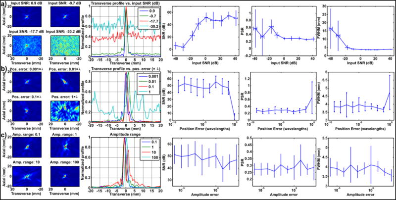
Acoustic modelling results for simulated 128 element 3D array. Effects of (a) noise (b) position error and (c) uneven element sensitivity. Columns show: selected acoustic maps for four values of the variable under test; transverse profile of the maps; the map signal to noise ratio (SNR), peak sidelobe ratio (PSR) and transverse full-width half maximum (FWHM).

Increasing levels of random noise (Fig. 4a) resulted in visible noise in the acoustic maps at high noise levels. However, this effect only became significant when the amplitude of the noise was greater than the signal (SNR < 0 dB). Below this point the SNR of the maps fell with the input SNR, but a focus was still clearly resolvable until around −20dB due to beamforming gain. Due to the increased level of noise in the maps the PSR and FWHM also increased at higher noise levels.

Small values of positioning error (Fig. 4b) below one wavelength had relatively little effect on the resulting maps, or on any of the derived parameters. Position errors of one wavelength or above were catastrophic due to destruction of signal coherence. It should be noted that the array elements were considered as point sensors in this simulation, and the beam pattern of real finite sensors may introduce secondary effects which were not accounted for in this basic model.

Sensitivity variance (Fig. 4c) produced some distortion in the shape of the maps due to variable biasing of the signals from different elements. This effect varied depending on how the randomly generated bias was distributed over the elements. As the beamforming process is primarily sensitive to phase, the effect of uneven element sensitivity was relatively minor compared to noise or position error, even when the amplitude of the signals varied by several orders of magnitude. In practice, such large variation in element sensitivity may become a greater issue than shown here due to dynamic range limitations of receiving hardware.

3.4. Point source localization

A summary of the point source localization experiment is shown in Fig. 5. The point source transmitter was manually moved in steps of approximately 1–2 mm using a MRI-compatible manual positioning stage. The signals received on the array at each position were reconstructed about each of the three principal planes, for movement about the X (elevational plane of array; R/L of MRI), Y (transverse plane of array; S/I of MRI), and Z (axial direction of array; A/P of MRI) axes. Example maps about the three principal planes are shown for movements about the three axes in Fig. 5a, c and e. The results are summarized in Fig. 5b, d and f which shows normalized profiles extracted from the maps at each position.

Figure 5.

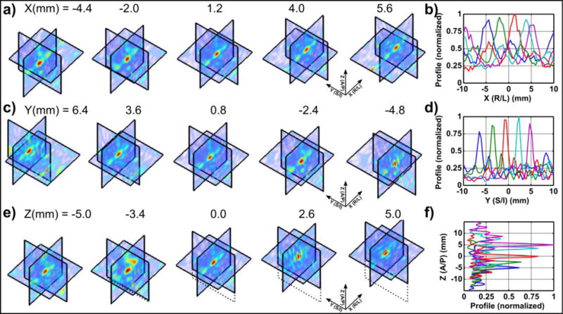
Point source localization results from 48 element 3D array. The transmitter was moved along the (a–b) X, (c–d) Y and (e–f) Z axes and maps reconstructed in a ±10 mm range about the 3 principal axes. (a, c, e) shows example maps about the 3 planes; (b, d f) shows profiles extracted from the maps, which were normalized with respect to the maximum value from all five profiles. The values of x, y, and z reported in (a, c, e) give the position of the peak in the acoustic maps when the source was moved in the corresponding direction.

3.5. Cavitation source localization

The results of the cavitation phantom experiment are shown in Fig. 6. RF data over each of the elements of the array is shown in Fig. 6a, for a sonication at 5 W without (left) and with (right) microbubbles. The data are averaged over the 60 s duration of sonication and shown before (top) and after (bottom) a 230 kHz notch filter to remove the excitation frequency (f₀). The data shows the transmit event during the first 50 μs, and returning echoes from the tube and water surface beginning at around 200 μs. This corresponds to the expected time for 300 mm round-trip distance at the speed of sound in water of 1.48 mm/μs. Before the filter, there is little obvious difference between the control and bubble sonications. After the filter the 230 kHz transmit burst is removed. The signal from the focal region was also removed by the filter in the control experiment, but not in the experiment with bubbles (red boxes). This suggests that the excess signal beginning at around 200 μs was created by the bubbles.

Figure 6.

Cavitation source experiment. A tube phantom containing water or microbubbles was sonicated with the therapy array and monitored using the 128-channel array. (a) RF data pre- (top) and post- notch filter (bottom), for control (left) and microbubble (right) experiments. (b) Average difference in spectra between the bubble and control experiments. The data were averaged over the array and sonication duration. (c) Amplitude of second harmonic over time. The sonication on-time is shown by the green overlay, and approximate start of manual microbubble injection by the black dashed line. (d) Representative 3D PAM for sonications with (top) and without (bottom) microbubbles. (e–f) Spatial peak, temporal sum value from PAM vs. (e) electrical power and (f) burst length. CW = continuous wave.

The difference in averaged frequency spectra between the two experiments is shown in Fig. 6b. Harmonics of the driving frequency (particularly at 2, 3 and 4 × f₀) and some increase in broadband noise are visible, suggesting microbubble activity.

The amplitude of the second harmonic over time is shown in Fig. 6c. The data were averaged over the elements of the array in the frequency domain. In the control experiment the amplitude of the signal was flat over the duration of sonication, while the microbubble experiment shows an obvious increase following microbubble injection which was maintained for the remainder of sonication. This further confirms that the changes in the RF data and frequency spectra were due to microbubble activity.

Representative acoustic maps for the two experiments are shown in Fig. 6d. The maps were constructed in a ±10 mm area about each of the 3 principal axes using a basic time domain delay and sum algorithm. The RF data were first filtered using a digital bandpass filter centered at 460 kHz (2 × f₀) and maps were summed over the duration of experiments. The same color scale was used to display the maps from the two experiments. Focal activity was clearly visible in the maps from the microbubble sonication (top) compared to the control sonication (bottom).

To illustrate the utility of the acoustic maps for monitoring cavitation activity the spatial peak, temporal sum value (i.e. max pixel value shown in the maps in Fig. 6d) was extracted as a function of the exposure conditions. Increasing the electrical power (Fig. 6e) showed simple linear behavior without microbubbles. With microbubbles, the amplitude of passive acoustic maps (PAM) increased by an order of magnitude compared to the control sonication, and increased non-linearly with electrical power due to microbubble behavior. Increasing the burst length had little effect in the control experiment apart from in the case of continuous wave (CW) sonication, suggesting onset of cavitation in absence of bubbles at high duty cycle. Increasing burst length also increased the PAM amplitude non-linearly due to increased bubble activity. For CW sonication, the amplitude fell, suggesting excessive microbubble destruction. The CW sonication also shows that the array was still able to detect cavitation during a long transmit burst.

3.6. In vivo imaging

A summary of the in vivo experiment is shown in Fig. 7. Illustrative MR temperature maps and anatomical images taken during and after treatment respectively are shown in Fig. 7a. The location of the focus is shown by the green arrow. Due to the low power used in these experiments focal heating was modest (~2–3°C), however the location of the focus was just visible above the noise floor in the images (Fig. 7a, left). The anatomical image taken after treatment shows a small lesion was produced at the focus as a result of cavitation activity (Fig. 7a, right). It should be noted that this experiment formed part of a larger study and so the anatomical images were taken after several further sonications were completed. The MR anatomical image thus represents a summation of the effects of several sonications.

Figure 7.

In vivo results using 48 element 3D array. (a) Left: MR temperature map acquired during sonication, showing low-level temperature rise that can occur during sonication with microbubbles (McDannold et al 2006); Right: T2*-weighted MRI acquired after treatment, showing a small lesion created at the focus induced by cavitation activity. Scale bar = 1cm. (b) Comparison of averaged spectra over the duration of sonications with and without microbubbles. The averaged spectra from a sonication with microbubbles was subtracted from that without. (c) Magnitude of the second harmonic over time with and without microbubble injection. The sonication on-time is shown by the green overlay, and approximate start of manual microbubble injection by the black dashed line. (d–e) Acoustic maps reconstructed over the three principal planes, integrated over the duration of sonications (d) with and (e) without microbubbles. The two sets of maps are shown in the same color scale.

Summaries of the acoustic data for sonications with and without microbubbles in the animal experiment are shown in Fig. 7b–e. Using microbubbles, the spectra show increased harmonics and broadband noise (Fig. 7b), while the second harmonic shows a clear increase on microbubble injection (Fig. 7c). These results are qualitatively similar to the tube phantom experiment. The spectra show an increase in higher-order harmonics compared to the phantom experiment, perhaps due to the higher microbubble concentration and rich vascular network of the brain vs. the single vessel tube phantom model. The increase in acoustic signal was smaller than the phantom experiment (~6–8dB vs. ~10–12dB) as this experiment used an earlier prototype of the array with 48 elements instead of the completed 128 element array. Passive acoustic maps showed increased focal activity using microbubbles (Fig. 7d) compared to the control experiment (Fig. 7e). It should be noted that the therapy burst length of 91 ms used in this experiment was far greater than the ~200 μs round trip time to the focus of the transducer; these results thus confirm that the array was able to detect cavitation during sonication and while the therapy array was still transmitting.

4. Discussion

In this study a 3D sparse array was designed for active and passive ultrasound imaging within a clinical MR guided focused ultrasound device.

In active mode, the rib-based array design was readily capable of 2D B-mode imaging of a human skull which was situated within the clinical focused ultrasound device in the bore of the MRI scanner. Segmentation of the skull from MR images showed good qualitative agreement with the envelope of the outer skull surface shown in the B-mode images as expected. Simultaneous ultrasound and MR imaging systems have been demonstrated before (Tang et al 2008, Curiel et al 2007, Arvanitis et al 2013, Petrusca et al 2013) however to the best of our knowledge this is the first example in which a concave array large enough to encompass a human skull was used, and directly rendered as a real-time B-mode image.

Expansion of the array to seven ‘ribs’ allowed full three-dimensional localization of the skull by registration of pre-treatment skull MR images to the treatment space using the ultrasound data. Skull registration using ultrasound imaging has been shown before based on skull CT images (O’Reilly et al 2016) within a benchtop prototype array system without therapeutic elements. Here we segmented the skull directly from MRI, avoiding the need for CT, and integrated our array with a commercially-available clinical MRgFUS device. The use of MR imaging to obtain the reference skull images that are then located using the ultrasound data was convenient for the InSightec clinical system, which is MR-compatible, and avoids the use of ionizing radiation. However, CT typically provides higher resolution images than MRI, and is more inherently suitable for measurement of bone as an X-ray based modality. In clinical practice it is likely that many patients would be given pre-operative CT anyway, since this provides information on acoustically important parameters such as skull density (Chang et al 2015). Overall, the skull localization results shown here are within the range of those reported previously – for example (O’Reilly et al 2016) showed errors in displacement and rotation on the order of 1.5 mm/1.5° (± ~0.5 mm/0.5°) for a 64-element array, which is similar to that shown here with 48 elements. Manual testing of the robustness of the algorithm showed that translation errors were much more readily corrected than rotation. As a consequence of the (approximately hemispherical) shape of the skull, rotation is inherently a more difficult problem to solve than translation: small rotations may have very little effect on the distance from the array elements, while symmetry (e.g. 180° flip) may result in convergence to an incorrect solution. To account for this problem here the maximum rotation allowed by the algorithm was constrained to reduce the solution space to a tractable range, in the same manner as previous work (O’Reilly et al 2016). The use of such a constrained solver would require a reasonable accurate (within a few mm) initial estimate of the skull position. For current MR-guided procedures this may be obtained directly from the MRI data. Without MRI, direct measurements of the skull position relative to the transducer may provide a sufficiently accurate initial guess of position, given the typical (~3–5 mm) thickness of the scalp (Hori et al 1972). The ability of our system to render 2D B-mode images could also aid in alignment by providing visual feedback of the current position guess relative to the ultrasound data within each rib of the array.

In passive mode, an in silico model was adapted from previous work using linear arrays (Coviello et al 2015) in order to evaluate the effects of various imperfections which may occur using a practical – in this case hand-built – array. Though the approach used here was relatively simple the model was sufficient to demonstrate the effects of varying levels of simulated electrical noise, element position uncertainty, and uneven element sensitivity. The effects of these parameters were shown both in the resulting acoustic maps as well as in derived parameters such as the signal to noise ratio, in a similar manner to previous work (Jones et al 2013). In practice, each of these factors may be controlled by careful consideration of the array design and signal processing – for example, noise may be reduced by use of shielded cabling and use of filters, while element sensitivity could be accounted for by calibration and/or selection of elements with similar sensitivity. Uncertainty in element position appeared to have the largest effects on the ability of the system to resolve a map, since inaccurate positioning may destroy the phase information on which the beamforming process relies. A more robust beamforming algorithm may be able to reduce the impact of array calibration uncertainties (Coviello et al 2015), while cross-validation of the element positions obtained by acoustic triangulation using another modality such as CT (O’Reilly et al 2016) or optical measurements could improve confidence in the array performance.

To evaluate the ability of the system to perform passive imaging a point source was manually moved within the field of view of the array using an MR-compatible positioning system. Passive acoustic maps reconstructed in three dimensions showed that the point source was clearly resolved over the background noise, and could be tracked in real time as it was moved along each of the principal axes in turn. The profiles of the acoustic maps extracted about the focus in each location showed only minor variation in the amplitude displayed in the maps for movements in the two transverse (X and Y) directions. For movement in the Y direction (along the ribs of the array) lower amplitude side lobes (0.39±0.06 normalized value) were visible in some locations, which is comparable to that shown in previous work (O’Reilly et al 2014). Movement in the X direction (between ribs) showed more significant side lobes (approaching the amplitude of the main lobe) due to the extreme sparsity of the array in that direction. This is a significant limitation of the array in its current form, as localization data in the X direction cannot be reliably interpreted since focal activity may be confused with side lobes. Improvements in the array design to address this limitation are discussed below. In the Z direction (axial / out of bowl) the source was still resolved but larger variation in the amplitude displayed in the maps was observed. This is likely a consequence of the simple beamforming method used here, which did not account for the sensitivity pattern of the array elements.

Having demonstrated that the array could locate an ideal point source the system was tested using commercial microbubbles in a flow phantom to assess its capability for monitoring cavitation activity. Analysis of the data received by the array showed that cavitation-like acoustic emissions (increased harmonics and broadband noise) could be detected in the presence of the microbubbles and monitored in real time during the experiment. Passive acoustic maps showed that focal cavitation activity could be clearly spatially resolved using the array, which was absent in the control experiment. Variation of the acoustic conditions used in sonication confirmed that the power of acoustic emissions resolved in the maps increased significantly in the presence of microbubbles. The amplitude of acoustic emissions reflected in the maps was found to vary with the electrical power or burst length supplied to the therapy transducer in the anticipated manner. Generally speaking, increasing electrical power or burst length was associated with increasing amplitude of acoustic emissions as expected. However, in the presence of cavitation activity – promoted here by injection of microbubbles – the amplitude of acoustic emissions increased by an order of magnitude compared to sonications under the same conditions without microbubbles. The amplitude of acoustic emissions in presence of microbubbles varied in a nonlinear fashion with electrical power or burst length due to the complex nature of cavitation phenomena (Leighton 1994) – for example, increasing pressure may increase the amplitude of cavitation emissions to a point, beyond which saturation and shielding effects become significant (Coussios and Roy 2008). These results illustrate the utility of the system for real-time monitoring and detection of cavitation during focused ultrasound therapy. It should be noted that the duty cycle used in this part of the study was very low (0.008 %) and as such MR thermometry would be insufficient to monitor treatment as a result of the negligible effect on temperature.

Finally, to assess the suitability of the array for in vivo experiments, the system was used to monitor sonication of brain targets in a nonhuman primate model. The acoustic emissions received by the array showed multiple harmonic peaks and increased broadband noise, which increased in amplitude following microbubble injection in a similar manner to previous work using linear arrays for 2D imaging (Arvanitis et al 2013). Reconstruction of acoustic maps in 3 dimensions showed that the emissions could be spatially resolved in three dimensions, while MR imaging conducted during and after treatment confirmed successful non-thermal lesion production. These results show that three-dimensional passive acoustic imaging may be conducted in nonhuman primate brain within a clinical MRgFUS system, and suggest that with sufficient refinement such a system could be used to conduct cavitation-driven therapies in the brain in combination with or even without MR imaging.

The study presented in this paper has several limitations which could be improved in future work. In active mode, the array was readily able to conduct both two-dimensional conventional B-mode imaging, as well as 3D pulse-echo imaging for skull localization, within the clinical MRgFUS device. While the primary focus of this study was to produce a system which was compatible with a clinical device, previous work utilizing prototype devices (or separate arrays for active imaging) suggests numerous avenues for improvement, for example by employing higher element counts, optimization of element positions, or use of more complex algorithms to recover more information from the data (O’Reilly et al 2016). With respect to passive imaging, the array was able to monitor the emissions from and reconstruct three dimensional acoustic maps for point sources, cavitating microbubbles in a flow phantom, and microbubble activity in the brain in nonhuman primates. The main limitation of the array in its current form for passive imaging is the presence of side lobes, particularly in the X (between rib) direction, which were most readily demonstrated in the point source experiment for displacements about the X axis (Fig. 5a). This is largely a consequence of the extreme sparsity of the array in that direction as a result of the rib-based design, which clusters the elements around seven X-coordinate values and does not cover the full available bowl surface in that direction. To address this limitation the array design could be modified to allow greater flexibility in the placement of elements, allowing a more random sampling of the space within the transducer (Jones et al 2013) as well as covering the whole available aperture. With reference to Fig. 1, perhaps the simplest modification to the existing design would be to increase the number of cross-braces between ribs and populate these with elements. Since the cross-braces are aligned with the X-axis of the array this would allow much greater flexibility in element position in this direction. To cover the full aperture, additional angled ribs could be added to the left and right sections of the bowl. Alternatively, the design could be revised completely, for example by replacing the ribs with a thin (acoustically transparent) plastic bowl allowing through-transmission in a similar manner to membrane hydrophones (Shotton et al 1980). To further improve flexibility in element placement the piezo elements could be replaced with PVDF film, allowing transmission of the therapy wave through the elements themselves, at the possible expense of SNR (Collin et al 2013, Coviello et al 2012, O’Reilly and Hynynen 2010). Electrically speaking our design was relatively simple, and did not include refinements which have featured in other work such as impedance matching, element backing, or incorporation of hardware filters or pre-amplifiers (O’Reilly and Hynynen 2010, Collin et al 2013, O’Reilly et al 2016), any of which could undoubtedly improve the performance of the system at the cost of increased complexity. While the array was designed to provide minimal obstruction of the elements of the therapy transducer, the presence of the ribs and elements within the transducer may still affect ultrasound propagation (for example due to reflections from the additional surfaces, or direct propagation from edges of therapy array tiles) which was not quantified as part of this study. MRI thermometry and hydrophone measurements with and without the array in situ would allow assessment of the effects on therapy transducer focusing (e.g. changes in peak negative pressure or peak temperature at the focus, or change in full-width half-maximum of the focal region in pressure or temperature). Additional limitations of this study include the point source transmitter and manual positioning system used in the localization experiment, which were not sufficient to allow quantitative comparison of the position information displayed in the acoustic data with an accurate external reference. Finally, with respect to the algorithms used, our approach to passive imaging made use of simple delay and sum beamforming, and made no attempt to compensate for the overlapping sensitivity patterns of the array elements in the concave array geometry. A more complete formulation could account for the angled beam pattern of each element to derive an appropriate apodization function (Haworth et al 2012) to individually scale the RF data for each location, while alternative beamforming algorithms could be employed to improve processing speed for real-time imaging (Arvanitis et al 2016) or provide improved tolerance to array calibration uncertainties (Coviello et al 2015).

5. Conclusions

In this study a 3D sparse array was designed for active and passive ultrasound imaging within a clinical MR guided focused ultrasound device. The array is capable of both B-mode imaging at 5 MHz for skull localization, as well as passive reception at the second harmonic of the therapy array for detection of cavitation and passive acoustic imaging. In active mode, the array was able to perform B-mode imaging and 3D localization of a human skull with close agreement to MR imaging. In passive mode, the array was able to locate a point source in 3D, produce 3-dimensional passive acoustic maps of cavitation in a flow phantom, and detect cavitation associated with microbubble activity in the brain in nonhuman primates. These results demonstrate a dual-mode array which is compatible with a clinical MRgFUS device and suggests such a device could be useful for planning, monitoring and assessment of cavitation-enhanced transcranial focused ultrasound therapy.

References

- Arvanitis C, Crake C, McDannold N, Clement G. Passive acoustic mapping with the angular spectrum method. IEEE Transactions on Medical Imaging. 2016;36:983–93. doi: 10.1109/TMI.2016.2643565. [DOI] [PMC free article] [PubMed] [Google Scholar]
- Arvanitis CD, Livingstone MS, McDannold N. Combined ultrasound and MR imaging to guide focused ultrasound therapies in the brain. Phys Med Biol. 2013;58:4749–61. doi: 10.1088/0031-9155/58/14/4749. [DOI] [PMC free article] [PubMed] [Google Scholar]
- Arvanitis CD, McDannold N. Integrated ultrasound and magnetic resonance imaging for simultaneous temperature and cavitation monitoring during focused ultrasound therapies. Med Phys. 2013;40:112901. doi: 10.1118/1.4823793. [DOI] [PMC free article] [PubMed] [Google Scholar]
- Arvanitis CD, Vykhodtseva N, Jolesz F, Livingstone M, McDannold N. Cavitation-enhanced nonthermal ablation in deep brain targets: feasibility in a large animal model. J Neurosurg. 2015;124:1450–9. doi: 10.3171/2015.4.JNS142862. [DOI] [PMC free article] [PubMed] [Google Scholar]
- Bjornsson CS, Oh SJ, Al-Kofahi YA, Lim YJ, Smith KL, Turner JN, De S, Roysam B, Shain W, Kim SJ. Effects of insertion conditions on tissue strain and vascular damage during neuroprosthetic device insertion. J Neural Eng. 2006;3:196–207. doi: 10.1088/1741-2560/3/3/002. [DOI] [PubMed] [Google Scholar]
- Chang WS, Jung HH, Zadicario E, Rachmilevitch I, Tlusty T, Vitek S, Chang JW. Factors associated with successful magnetic resonance-guided focused ultrasound treatment: efficiency of acoustic energy delivery through the skull. J Neurosurg. 2015;124:411–6. doi: 10.3171/2015.3.JNS142592. [DOI] [PubMed] [Google Scholar]
- Clement GT, Hynynen K. A non-invasive method for focusing ultrasound through the human skull. Phys Med Biol. 2002;47:1219. doi: 10.1088/0031-9155/47/8/301. [DOI] [PubMed] [Google Scholar]
- Cline HE, Schenck JF, Hynynen K, Watkins RD, Souza SP, Jolesz FA. MR-Guided Focused Ultrasound Surgery. J Comput Assist Tomogr. 1992;16:956. doi: 10.1097/00004728-199211000-00024. [DOI] [PubMed] [Google Scholar]
- Collin J, Coviello C, Lyka E, Leslie T, Coussios CC. Real-time three-dimensional passive cavitation detection for clinical high intensity focussed ultrasound systems. Proc Meet Acoust. 2013;19:075023. [Google Scholar]
- Coussios C-C, Farny CH, ter Haar G, Roy RA. Role of acoustic cavitation in the delivery and monitoring of cancer treatment by high-intensity focused ultrasound (HIFU) Int J Hyperthermia. 2007;23:105–20. doi: 10.1080/02656730701194131. [DOI] [PubMed] [Google Scholar]
- Coussios C-C, Roy RA. Applications of Acoustics and Cavitation to Noninvasive Therapy and Drug Delivery. Annu Rev Fluid Mech. 2008;40:395–420. [Google Scholar]
- Coviello C, Kozick R, Choi J, Gyöngy M, Jensen C, Smith PP, Coussios C-C. Passive acoustic mapping utilizing optimal beamforming in ultrasound therapy monitoring. J Acoust Soc Am. 2015;137:2573–85. doi: 10.1121/1.4916694. [DOI] [PubMed] [Google Scholar]
- Coviello CM, Kozick RJ, Hurrell A, Smith PP, Coussios C. Thin-film sparse boundary array design for passive acoustic mapping during ultrasound therapy. IEEE Trans Ultrason Ferroelectr Freq Control. 2012;59:2322–30. doi: 10.1109/TUFFC.2012.2457. [DOI] [PubMed] [Google Scholar]
- Crake C, Meral FC, Burgess MT, Papademetriou IT, McDannold NJ, Porter TM. Combined passive acoustic mapping and magnetic resonance thermometry for monitoring phase-shift nanoemulsion enhanced focused ultrasound therapy. Phys Med Biol. 2017;62:6144–63. doi: 10.1088/1361-6560/aa77df. [DOI] [PMC free article] [PubMed] [Google Scholar]
- Crake C, Owen J, Smart S, Coviello C, Coussios C-C, Carlisle R, Stride E. Enhancement and Passive Acoustic Mapping of Cavitation from Fluorescently Tagged Magnetic Resonance-Visible Magnetic Microbubbles In Vivo. Ultrasound Med Biol. 2016;42:3022–3036. doi: 10.1016/j.ultrasmedbio.2016.08.002. [DOI] [PubMed] [Google Scholar]
- Crake C, de Saint Victor M, Owen J, Coviello C, Collin J, Coussios C-C, Stride E. Passive acoustic mapping of magnetic microbubbles for cavitation enhancement and localization. Phys Med Biol. 2015;60:785–806. doi: 10.1088/0031-9155/60/2/785. [DOI] [PubMed] [Google Scholar]
- Curiel L, Chopra R, Hynynen K. Progress in Multimodality Imaging: Truly Simultaneous Ultrasound and Magnetic Resonance Imaging. Ieee Trans Med Imaging. 2007;26:1740–6. doi: 10.1109/tmi.2007.903572. [DOI] [PMC free article] [PubMed] [Google Scholar]
- Deng L, O’Reilly MA, Jones RM, An R, Hynynen K. A multi-frequency sparse hemispherical ultrasound phased array for microbubble-mediated transcranial therapy and simultaneous cavitation mapping. Phys Med Biol. 2016;61:8476. doi: 10.1088/0031-9155/61/24/8476. [DOI] [PMC free article] [PubMed] [Google Scholar]
- Dillon C, Roemer R, Payne A. Quantifying perfusion-related energy losses during magnetic resonance-guided focused ultrasound. J Ther Ultrasound. 2015;3:O103. [Google Scholar]
- Elias WJ, Lipsman N, Ondo WG, Ghanouni P, Kim YG, Lee W, Schwartz M, Hynynen K, Lozano AM, Shah BB, Huss D, Dallapiazza RF, Gwinn R, Witt J, Ro S, Eisenberg HM, Fishman PS, Gandhi D, Halpern CH, Chuang R, Butts Pauly K, Tierney TS, Hayes MT, Cosgrove GR, Yamaguchi T, Abe K, Taira T, Chang JW. A Randomized Trial of Focused Ultrasound Thalamotomy for Essential Tremor. N Engl J Med. 2016;375:730–9. doi: 10.1056/NEJMoa1600159. [DOI] [PubMed] [Google Scholar]
- Escoffre J-M, Bouakaz A. Therapeutic Ultrasound. Springer: 2015. [Google Scholar]
- Gyöngy M, Coussios CC. Passive Spatial Mapping of Inertial Cavitation During HIFU Exposure. IEEE Trans Biomed Eng. 2010a;57:48–56. doi: 10.1109/TBME.2009.2026907. [DOI] [PubMed] [Google Scholar]
- Gyöngy M, Coussios C-C. Passive cavitation mapping for localization and tracking of bubble dynamics. J Acoust Soc Am. 2010b;128:EL175–EL180. doi: 10.1121/1.3467491. [DOI] [PubMed] [Google Scholar]
- ter Haar G, Coussios C. High intensity focused ultrasound: Physical principles and devices. Int J Hyperthermia. 2007;23:89–104. doi: 10.1080/02656730601186138. [DOI] [PubMed] [Google Scholar]
- Haworth KJ, Mast TD, Radhakrishnan K, Burgess MT, Kopechek JA, Huang S-L, McPherson DD, Holl CK. Passive imaging with pulsed ultrasound insonations. J Acoust Soc Am. 2012;132:544–53. doi: 10.1121/1.4728230. [DOI] [PMC free article] [PubMed] [Google Scholar]
- Hölscher T, Fisher D, Raman R. Noninvasive Transcranial Clot Lysis Using High Intensity Focused Ultrasound. J Neurol Neurophysiol. 2011;01 Online: http://www.omicsonline.org/2155-9562/2155-9562-S1-002.php. [Google Scholar]
- Hori H, Moretti G, Rebora A, Crovato F. The Thickness of Human Scalp: Normal and Bald. J Invest Dermatol. 1972;58:396–9. doi: 10.1111/1523-1747.ep12540633. [DOI] [PubMed] [Google Scholar]
- Hynynen K, Clement G. Clinical applications of focused ultrasound—The brain. Int J Hyperthermia. 2007;23:193–202. doi: 10.1080/02656730701200094. [DOI] [PubMed] [Google Scholar]
- Hynynen K, Jolesz FA. Demonstration of potential noninvasive ultrasound brain therapy through an intact skull. Ultrasound Med Biol. 1998;24:275–83. doi: 10.1016/s0301-5629(97)00269-x. [DOI] [PubMed] [Google Scholar]
- Hynynen K, McDannold N. MRI guided and monitored focused ultrasound thermal ablation methods: a review of progress. Int J Hyperthermia. 2004;20:725–37. doi: 10.1080/02656730410001716597. [DOI] [PubMed] [Google Scholar]
- Hynynen K, McDannold N, Sheikov NA, Jolesz FA, Vykhodtseva N. Local and reversible blood—brain barrier disruption by noninvasive focused ultrasound at frequencies suitable for trans-skull sonications. NeuroImage. 2005;24:12–20. doi: 10.1016/j.neuroimage.2004.06.046. [DOI] [PubMed] [Google Scholar]
- Hynynen K, McDannold N, Vykhodtseva N, Jolesz FA. Noninvasive MR Imaging—guided Focal Opening of the Blood-Brain Barrier in Rabbits. Radiology. 2001;220:640–6. doi: 10.1148/radiol.2202001804. [DOI] [PubMed] [Google Scholar]
- InSightec. ExAblate® Model 4000 Type 1 Application: Brain Essential Tremor: Information for prescribers. 2016 System Software Version 6.6. FDA Submission July 2016 Online: http://www.accessdata.fda.gov/cdrh_docs/pdf15/P150038C.pdf.
- Ishihara Y, Calderon A, Watanabe H, Okamoto K, Suzuki Y, Kuroda K, Suzuki Y. A precise and fast temperature mapping using water proton chemical shift. Magn Reson Med. 1995;34:814–23. doi: 10.1002/mrm.1910340606. [DOI] [PubMed] [Google Scholar]
- Jones RM, O’Reilly MA, Hynynen K. Transcranial passive acoustic mapping with hemispherical sparse arrays using CT-based skull-specific aberration corrections: a simulation study. Phys Med Biol. 2013;58:4981–5005. doi: 10.1088/0031-9155/58/14/4981. [DOI] [PMC free article] [PubMed] [Google Scholar]
- Khokhlova VA, Bailey MR, Reed JA, Cunitz BW, Kaczkowski PJ, Crum LA. Effects of nonlinear propagation, cavitation, and boiling in lesion formation by high intensity focused ultrasound in a gel phantom. J Acoust Soc Am. 2006;119:1834–48. doi: 10.1121/1.2161440. [DOI] [PubMed] [Google Scholar]
- Lehr HA, Mankoff DA, Corwin D, Santeusanio G, Gown AM. Application of photoshop-based image analysis to quantification of hormone receptor expression in breast cancer. Journal of Histochemistry & Cytochemistry. 1997;45:1559–1565. doi: 10.1177/002215549704501112. [DOI] [PubMed] [Google Scholar]
- Lee JY, Crake C, Teo B, Carugo D, de Saint Victor M, Seth A, Stride E. Ultrasound-enhanced siRNA delivery using magnetic nanoparticle-loaded chitosan-deoxycholic acid nanodroplets. Adv Healthc Mater. 2017:1–20. doi: 10.1002/adhm.201601246. [DOI] [PubMed] [Google Scholar]
- Leighton TG. The Acoustic Bubble. London: Academic Press; 1994. [Google Scholar]
- Leinenga G, Langton C, Nisbet R, Götz J. Ultrasound treatment of neurological diseases—current and emerging applications. Nat Rev Neurol. 2016;12:161–74. doi: 10.1038/nrneurol.2016.13. [DOI] [PubMed] [Google Scholar]
- Lipsman N, Schwartz ML, Huang Y, Lee L, Sankar T, Chapman M, Hynynen K, Lozano AM. MR-guided focused ultrasound thalamotomy for essential tremor: a proof-of-concept study. Lancet Neurol. 2013;12:462–468. doi: 10.1016/S1474-4422(13)70048-6. [DOI] [PubMed] [Google Scholar]
- Maroon JC, Onik G, Quigley MR, Bailes JE, Wilberger JE, Kennerdell JS. Cryosurgery re-visited for the removal and destruction of brain, spinal and orbital tumours. Neurol Res. 1992;14:294–302. doi: 10.1080/01616412.1992.11740073. [DOI] [PubMed] [Google Scholar]
- McDannold N, Clement G, Black P, Jolesz F, Hynynen K. Transcranial MRI-guided focused ultrasound surgery of brain tumors: Initial findings in three patients. Neurosurgery. 2010;66:323. doi: 10.1227/01.NEU.0000360379.95800.2F. [DOI] [PMC free article] [PubMed] [Google Scholar]
- McDannold NJ, Vykhodtseva NI, Hynynen K. Microbubble Contrast Agent with Focused Ultrasound to Create Brain Lesions at Low Power Levels: MR Imaging and Histologic Study in Rabbits 1. Radiology. 2006;241:95–106. doi: 10.1148/radiol.2411051170. [DOI] [PubMed] [Google Scholar]
- Miller DL, Thomas RM. Contrast-agent gas bodies enhance hemolysis induced by lithotripter shock waves and high-intensity focused ultrasound in whole blood. Ultrasound Med Biol. 1996;22:1089–95. doi: 10.1016/s0301-5629(96)00126-3. [DOI] [PubMed] [Google Scholar]
- Myers R, Coviello C, Erbs P, Foloppe J, Rowe C, Kwan J, Crake C, Finn S, Jackson E, Balloul J-M, Story C, Coussios C, Carlisle R. Polymeric Cups for Cavitation-mediated Delivery of Oncolytic Vaccinia Virus. Molecular Therapy. 2016;24:1627–33. doi: 10.1038/mt.2016.139. [DOI] [PMC free article] [PubMed] [Google Scholar]
- Odéen H, de Bever J, Almquist S, Farrer A, Todd N, Payne A, Snell JW, Christensen DA, Parker DL. Treatment envelope evaluation in transcranial magnetic resonance-guided focused ultrasound utilizing 3D MR thermometry. J Ther Ultrasound. 2014;2:19. doi: 10.1186/2050-5736-2-19. [DOI] [PMC free article] [PubMed] [Google Scholar]
- O’Reilly MA, Hynynen K. A PVDF receiver for ultrasound monitoring of transcranial focused ultrasound therapy. IEEE Trans Biomed Eng. 2010;57:2286–2294. doi: 10.1109/TBME.2010.2050483. [DOI] [PMC free article] [PubMed] [Google Scholar]
- O’Reilly MA, Jones RM, Birman G, Hynynen K. Registration of human skull computed tomography data to an ultrasound treatment space using a sparse high frequency ultrasound hemispherical array. Med Phys. 2016;43:5063–71. doi: 10.1118/1.4960362. [DOI] [PMC free article] [PubMed] [Google Scholar]
- O’Reilly MA, Jones RM, Hynynen K. Three-Dimensional Transcranial Ultrasound Imaging of Microbubble Clouds Using a Sparse Hemispherical Array. Biomed Eng IEEE Trans On. 2014;61:1285–94. doi: 10.1109/TBME.2014.2300838. [DOI] [PMC free article] [PubMed] [Google Scholar]
- Petrusca L, Cattin P, De Luca V, Preiswerk F, Celicanin Z, Auboiroux V, Viallon M, Arnold P, Santini F, Terraz S, Scheffler K, Becker CD, Salomir R. Hybrid ultrasound/magnetic resonance simultaneous acquisition and image fusion for motion monitoring in the upper abdomen. Invest Radiol. 2013;48:333–40. doi: 10.1097/RLI.0b013e31828236c3. [DOI] [PubMed] [Google Scholar]
- Poliachik SL, Chandler WL, Mourad PD, Bailey MR, Bloch S, Clevel RO, Kaczkowski P, Keilman G, Porter T, Crum LA. Effect of high-intensity focused ultrasound on whole blood with and without microbubble contrast agent. Ultrasound Med Biol. 1999;25:991–8. doi: 10.1016/s0301-5629(99)00043-5. [DOI] [PubMed] [Google Scholar]
- Rapoport NY, Kennedy AM, Shea JE, Scaife CL, Nam K-H. Controlled and targeted tumor chemotherapy by ultrasound-activated nanoemulsions/microbubbles. J Controlled Release. 2009;138:268–76. doi: 10.1016/j.jconrel.2009.05.026. [DOI] [PMC free article] [PubMed] [Google Scholar]
- Rieke V, Butts Pauly K. MR thermometry. J Magn Reson Imaging. 2008;27:376–90. doi: 10.1002/jmri.21265. [DOI] [PMC free article] [PubMed] [Google Scholar]
- Salgaonkar VA, Datta S, Holl CK, Mast TD. Passive cavitation imaging with ultrasound arrays. J Acoust Soc Am. 2009;126:3071–83. doi: 10.1121/1.3238260. [DOI] [PMC free article] [PubMed] [Google Scholar]
- Sheeran PS, Dayton PA. Phase-change contrast agents for imaging and therapy. Curr Pharm Des. 2012;18:2152–65. doi: 10.2174/138161212800099883. [DOI] [PMC free article] [PubMed] [Google Scholar]
- Shotton KC, Bacon DR, Quilliam RM. A PVDF membrane hydrophone for operation in the range 0.5 MHz to 15 MHz. Ultrasonics. 1980;18:123–126. doi: 10.1016/0041-624x(80)90025-6. [DOI] [PubMed] [Google Scholar]
- Tang AM, Kacher DF, Lam EY, Wong KK, Jolesz FA, Yang ES. Simultaneous ultrasound and MRI system for breast biopsy: compatibility assessment and demonstration in a dual modality phantom. IEEE Trans Med Imaging. 2008;27:247–54. doi: 10.1109/TMI.2007.911000. [DOI] [PubMed] [Google Scholar]
- Vimeux FC, De Zwart JA, Palussiére J, Fawaz R, Delalande C, Canioni P, Grenier N, Moonen CTW. Real-Time Control of Focused Ultrasound Heating Based on Rapid MR Thermometry. Invest Radiol. 1999;34:190–193. doi: 10.1097/00004424-199903000-00006. [DOI] [PubMed] [Google Scholar]
- Vokurka K. A method for evaluating experimental data in bubble dynamics studies. Czechoslov J Phys B. 1986;36:600–15. [Google Scholar]
- Vokurka K. Experimental study of the bubble pulse. Acustica. 1988;66:174–176. [Google Scholar]
- Vokurka K. Cavitation noise modeling and analyzing CD-ROM Proceedings of Forum Acousticum 2002. Sociedad Espanola de Acustica; 2002. 2002. [Google Scholar]
- Zhang P, Porter T. An in vitro study of a phase-shift nanoemulsion: a potential nucleation agent for bubble-enhanced HIFU tumor ablation. Ultrasound Med Biol. 2010;36:1856–66. doi: 10.1016/j.ultrasmedbio.2010.07.001. [DOI] [PubMed] [Google Scholar]
- Zhang S, Ding T, Wan M, Jiang H, Yang X, Zhong H, Wang S. Minimizing the thermal losses from perfusion during focused ultrasound exposures with flowing microbubbles. J Acoust Soc Am. 2011;129:2336–44. doi: 10.1121/1.3552982. [DOI] [PubMed] [Google Scholar]